A Method for Super-Resolution Reconstruction of Marine Geomagnetic Anomaly Reference Maps Based on an Improved Generative Adversarial Network

Abstract

High-resolution marine geomagnetic anomaly maps are a prerequisite for accurate geomagnetic matching navigation. However, existing compilations are sparse and of low resolution, and conventional interpolation techniques fail to capture fine-scale anomalies. Although deep learning models have achieved remarkable success in natural-image super-resolution, they have rarely been tailored to geomagnetic grid data; their lack of physically motivated constraints frequently introduces geologically implausible structures. To address these limitations, we propose a physics-constrained generative adversarial network (PC-GAN) for the super-resolution reconstruction of marine geomagnetic anomaly maps. Building upon the Super-Resolution Generative Adversarial Network (SRGAN) backbone, we incorporate physics-informed loss terms for spatial continuity and edge preservation into the training objective, thereby endowing the data-driven architecture with geological consistency while maintaining numerical accuracy. Experiments were conducted on the NOAA EMAG2_V3 dataset across four representative marine regions. Over the Philippine Sea Plate, PC-GAN reduces the root-mean-square error (RMSE) by 28.0% and increases the peak signal-to-noise ratio (PSNR) by 2.85 dB relative to bicubic interpolation, and lowers RMSE by 27.5% while raising PSNR by 2.79 dB compared with PSO-Kriging. Ablation studies corroborate that the physics-based modules make a statistically significant contribution to reconstruction quality. PC-GAN furnishes a robust tool for generating high-fidelity geomagnetic reference maps and holds promise for high-precision geomagnetic matching navigation and related applications.

1. Introduction

As an inherent physical field of the Earth system, the geomagnetic field holds irreplaceable application value in areas including marine navigation, geological exploration, and environmental monitoring [1,2]. In recent years, with the widespread adoption of autonomous underwater vehicles (AUVs) and unmanned surface vessels (USVs), the demand for satellite-independent navigation technologies has surged. Geomagnetic matching navigation, leveraging its strengths of strong anti-interference capability and no cumulative errors, has emerged as a key supplement to marine autonomous navigation systems, and high-resolution, high-precision geomagnetic data is one of the critical prerequisites for achieving high-precision geomagnetic matching navigation [3]. Currently, the primary approaches to acquiring geomagnetic field data encompass satellite magnetic surveys, ground-based station observations, and aerial magnetic surveys. Satellite magnetic survey missions, including ESA’s Swarm constellation and the U.S. MAGSAT satellite, provide global-scale magnetic field coverage. The models released through these missions, including the International Geomagnetic Reference Field (IGRF) and CHAMP Satellite Mission (CHAMP), provide geomagnetic field information at a resolution of roughly 100 km. However, due to limitations in satellite payload accuracy and orbital altitude, they struggle to capture detailed local geomagnetic characteristics [4,5,6]. By deploying devices like fluxgate magnetometers and superconducting quantum interferometers, ground stations are capable of acquiring real-time magnetic field data with an accuracy down to the nT level. Nevertheless, the distribution of these stations is limited by geographical factors, resulting in observation blind spots in areas such as polar regions and deep oceans [7]. Aeromagnetic surveys, which utilize aircraft equipped with proton magnetometers, can achieve high-resolution (50–100 m) magnetic measurements in key zones. Yet, due to flight costs and weather conditions, the feasibility of large-scale, full-area surveys remains relatively low [8]. Data acquired via the above-mentioned approaches all suffer from sparsity and uneven distribution. However, applications including geomagnetic matching navigation and marine geological inversion demand continuous, high-precision geomagnetic data. It is therefore essential to reconstruct a continuous geomagnetic field from discrete data using diverse methods. Notably, constructing high-precision geomagnetic data from sparse, discrete observational data serves as a critical prerequisite for applications in fields like geomagnetic matching navigation and marine exploration.

In recent years, deep learning technologies, particularly generative adversarial networks, have achieved remarkable breakthroughs in image super-resolution reconstruction and offer a promising solution for the super-resolution reconstruction of geomagnetic anomalous fields [9,10]. A GAN consists of a generator and a discriminator, both of which are continuously optimized through adversarial training: the generator aims to produce realistic high-resolution images to “deceive” the discriminator, while the discriminator works to distinguish between real high-resolution images and those generated by the generator. This adversarial mechanism enables GANs to excel at generating high-resolution images with rich details and textures.

In the field of remote sensing image super-resolution, GANs have been widely applied. For instance, Li et al. [11] proposed a novel GAN framework for remote sensing image super-resolution reconstruction, addressing the limitations of traditional GANs in generating high-frequency details and realistic textures. Kong and Zhong [12] developed RGSRGAN, which captures long-range pixel dependencies via recursive gated convolution and leverages implicit adversarial loss to enhance the detail expression of reconstructed images. These studies demonstrate that GANs can effectively improve the spatial resolution of remote sensing images, providing technical insights for the high-fidelity reconstruction of geomagnetic anomalous fields. Wang et al. [13] introduced a multi-scale attention-guided GAN that adaptively emphasizes edge-rich regions, significantly suppressing aliasing artifacts in heterogeneous land-cover scenes. Montagnon et al. [14] embedded physical priors derived from the modulation transfer function into the adversarial loss, yielding sub-pixel accuracy consistent with satellite optical characteristics.

Despite the progress made in geomagnetic field modeling and super-resolution reconstruction, three limitations remain evident. From the data perspective, existing satellite and aeromagnetic compilations are generally coarser than 3 km in spatial resolution, and ship-track coverage is extremely sparse in deep-ocean regions; consequently, fine-scale anomaly features are missing and cannot satisfy the meter-level accuracy required by geomagnetic matching navigation. Methodologically, conventional interpolation schemes assume spatial continuity but rely on linear models, making it difficult to recover high-frequency nonlinear anomalies associated with seafloor structures; although deep learning approaches can learn nonlinear mappings, they have been developed primarily for natural images and lack explicit constraints on basic potential-field principles such as continuity and the absence of negative anomalies in source-free regions, easily producing spurious high or negative values in data-poor areas and degrading the reliability of navigation matching. In terms of validation, previous studies have usually focused on a single basin, lack cross-tectonic comparisons, and seldom report the model’s generalization error or computational cost outside the training swath, limiting the practical usability of these methods in real-world geomagnetic matching navigation. Therefore, how to reconstruct high-precision, high-resolution geomagnetic anomaly maps from sparse, low-resolution observations over large marine areas remains an urgent and unresolved research gap.

For super-resolution reconstruction of marine geomagnetic anomaly fields, traditional interpolation methods inevitably induce blurring and detail loss owing to their algorithmic simplicity, thereby failing to meet the stringent requirements of fine-scale geological interpretation [15]. Physics-driven modeling approaches achieve reasonable fidelity for global field recovery but exhibit limited capacity in capturing localized, high-frequency anomalies imposed by complex seafloor structures [16]. Data-driven deep learning strategies, most notably convolutional neural networks, although capable of learning nonlinear mappings, have predominantly been optimized for natural images; when directly transferred to geomagnetic grids they tend to generate overly smoothed outputs and disregard fundamental potential-field constraints such as spatial continuity and the absence of negative anomalies in source-free regions [17]. These observed shortcomings underscore three persistent limitations. First, from a data perspective: existing satellite and aeromagnetic compilations rarely exceed 3 km spatial resolution [18], while ship-track coverage remains extremely sparse in deep-ocean basins, resulting in a widespread deficit of meter-level anomaly details indispensable for high-precision geomagnetic matching navigation. Second, methodologically: conventional schemes rely on linear or weakly nonlinear spatial assumptions, whereas current deep learning architectures lack physics-informed regularization, frequently producing spurious extrema in data-poor areas and consequently degrading navigation reliability [19,20]. Third, in terms of validation: prior studies have typically focused on a single tectonic province, neglected cross-basin generalization assessment, and rarely reported computational overhead or predictive uncertainty beyond the training swath, collectively constraining their operational utility for autonomous platforms. Consequently, the development of a reconstruction framework that jointly enforces numerical fidelity and geophysical consistency while operating on sparse, low-resolution observations across broad marine domains remains an open and critical research gap.

To address the aforementioned challenges, we propose a physics-constrained generative adversarial network (PC-GAN) that enables high-fidelity super-resolution reconstruction of marine geomagnetic anomaly maps. The key contributions of this work are summarized as follows:

1.

A multi-objective optimization framework that jointly enforces pixel-level accuracy via RMSE, adversarial realism and physics-informed constraints of spatial continuity and edge preservation, ensuring both numerical precision and geophysical consistency.

2.

A PC-GAN architecture built upon SRGAN and specifically tailored to geomagnetic grids, incorporating dedicated continuity and edge-preservation loss terms to suppress artifacts and recover seafloor-structure-related high-frequency anomalies.

3.

Comprehensive validation over four tectonically distinct marine regions using the NOAA EMAG2_V3 dataset; PC-GAN reduces RMSE by up to 28% and increases PSNR by approximately 2.8 dB relative to bicubic and PSO-Kriging baselines, while ablation experiments quantitatively verify the individual and synergistic benefits of the physics-based modules.

2. Methods

The previous section has systematically outlined the practical demands for super-resolution reconstruction of marine geomagnetic anomaly reference maps. Existing data are characterized by low resolution and sparse distribution. Traditional interpolation methods fail to capture fine-scale anomaly features, and conventional deep learning models lack physical constraints, which easily leads to the generation of geologically implausible structures. To address these core challenges, this chapter will elaborate on the technical architecture of the proposed PC-GAN. From two dimensions, namely network design and loss function construction, it will illustrate how to achieve high-fidelity super-resolution reconstruction of geomagnetic data by integrating the physical properties of the geomagnetic field with adversarial learning mechanisms.

2.1. Physics-Constrained Generative Adversarial Network Architecture Design

Super-Resolution Generative Adversarial Network (SRGAN) serves as a classic paradigm for data-driven image super-resolution reconstruction. It addresses the inherent issues of excessive smoothing and low texture fidelity in high-resolution detail recovery that plague traditional interpolation methods by leveraging the adversarial learning mechanism between the generator and the discriminator, thereby establishing the core architectural foundation for advancing subsequent image super-resolution models. Compared with approaches like SRCNN, which rely on pixel-level error minimization, SRGAN incorporates adversarial learning to generate high-resolution images that align better with human visual perception. This enables it to demonstrate notable advantages in super-resolution tasks involving natural images, remote sensing images, and beyond. However, in super-resolution scenarios demanding high spatial continuity and authentic detail textures, the inherent architectural design of conventional SRGAN still exhibits limitations in preserving complex textures and suppressing artifacts [21].

As Earth’s inherent physical field, the geomagnetic field, characterized by its distinct composition and properties, constitutes the core foundation of geomagnetic matching navigation technology. From a physical perspective, it can be expressed as:

$$B=B_0+B_a+B_d$$

(1)

where B₀ denotes the main geomagnetic field. It is primarily generated by the Earth’s core and has gentle spatial variations. B_a represents the geomagnetic anomalous field. It originates from crustal magnetic materials and has stable temporal characteristics as well as rich spatial details. B_d stands for the disturbing magnetic field. It usually comes from the ionosphere or magnetosphere and causes observational errors. The three components differ significantly in their origins and properties [22]. For geomagnetic matching navigation, the main magnetic field exhibits only gentle spatial variations, which fail to provide sufficient positional discrimination. Meanwhile, the temporal instability of interfering magnetic fields introduces observational errors. In contrast, the anomalous field, characterized by its temporal stability and rich spatial detail, fully satisfies the core requirements for reference data. When a carrier operates near the Earth’s surface, variations in the geomagnetic field intensity it perceives are primarily driven by the geomagnetic anomalous field [23]. Thus, geomagnetic anomaly maps, which characterize the properties of the geomagnetic anomalous field, inherently qualify as reference data for geomagnetic matching navigation. This explains why the present study employs geomagnetic anomalous field data for super-resolution reconstruction.

The PC-GAN proposed in this study builds on the architectural framework of the Super-Resolution Generative Adversarial Network (SRGAN). Tailored to the technical needs of super-resolution reconstruction for marine geomagnetic anomaly reference maps, it enables accurate reconstruction of low-resolution (LR) geomagnetic data into high-resolution (HR) geomagnetic data by incorporating unique physical constraints inherent to geomagnetic anomaly fields. At the core of its design is the retention of the classic adversarial collaboration framework between the generator and discriminator in Generative Adversarial Networks (GANs). Specifically, long skip connections are added between generator layers to mitigate the vanishing gradient problem [24]; gradient penalty is employed in the discriminator to enhance training stability [25]; and a composite loss function with multi-dimensional constraints is innovatively introduced. In detail, the content loss guarantees that the reconstructed anomalies preserve the amplitude range observed in marine magnetic surveys; the spatial-continuity loss penalizes abrupt pixel-wise variations, mirroring the inherent smoothness of crustal magnetic potentials; the edge-preservation loss, computed with Sobel gradients, retains the sharp anomaly boundaries produced by geological contacts or fault structures. Finally, the feature-matching loss guides the generator to reproduce the spectral statistics of real geomagnetic grids, preventing the spectral flattening typical of SRGAN-based super-resolution that was originally designed for natural photographs rather than potential-field data. Through this multi-objective, physics-informed optimization strategy, the network simultaneously attains numerical fidelity and geophysical consistency (see Figure 1).

2.1.1. Generator Architecture

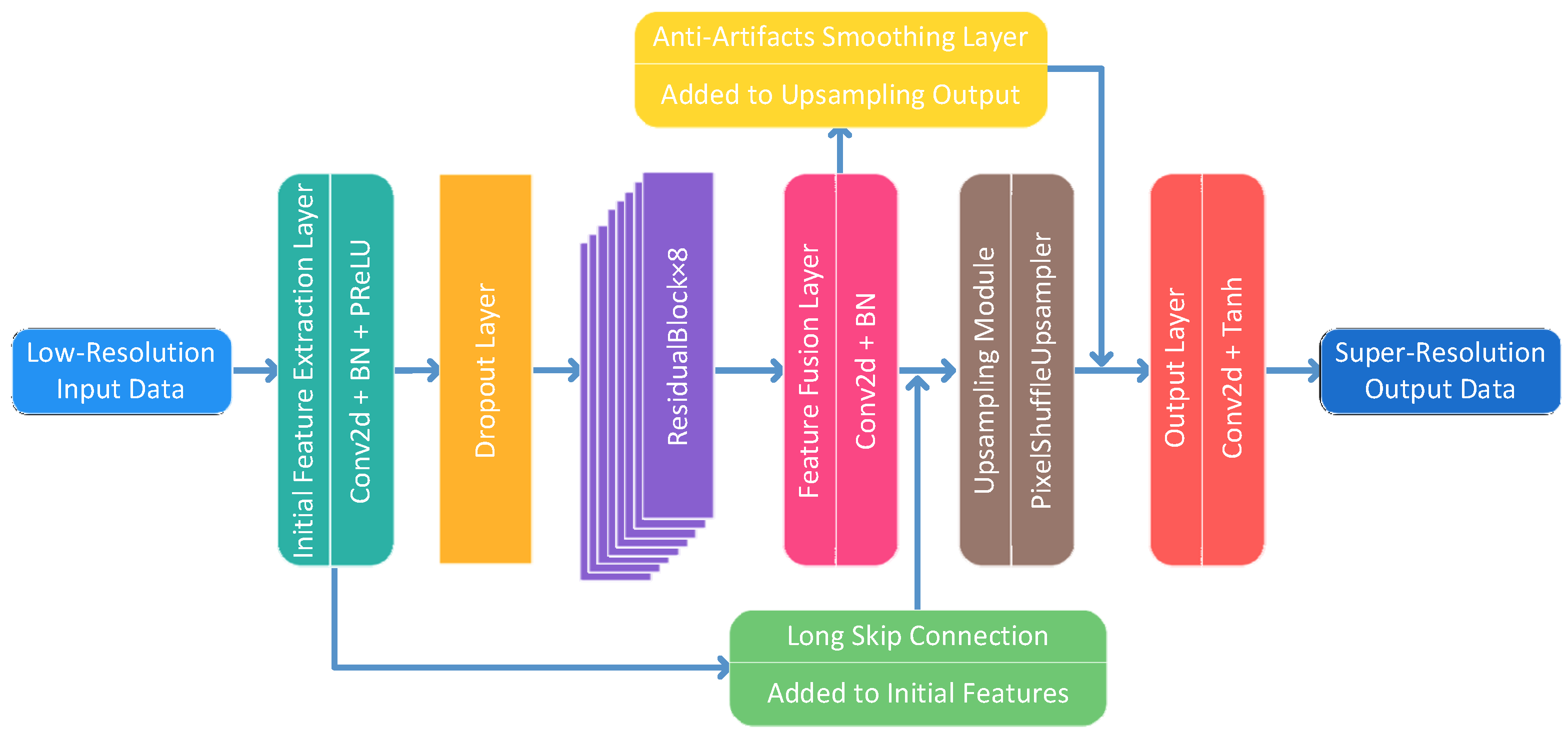
The generator adopts a “feature extraction-residual enhancement-feature fusion-upsampling” framework, comprising 8 improved residual blocks and an upsampling module. Its architecture is illustrated in Figure 2.

The generator accepts 32 × 32 resolution low-resolution(LR) geomagnetic grid data as input. First, an initial feature extraction module composed of a 3 × 3 convolutional layer (64 output channels), a batch normalization (BatchNorm2d) layer, a Parametric Rectified Linear Unit (PReLU) activation function, and a Dropout layer optimizes the initial feature mapping. Next, the feature map is fed into a residual learning module formed by eight improved residual blocks stacked in series. This module also incorporates global skip connections to fuse initial and deep features, mitigating the vanishing gradient issue [18]. Subsequently, the enhanced feature map is refined via an anti-artifact smoothing layer before entering a PixelShuffle-based upsampling module. It first expands channels using a 3 × 3 convolution, then achieves lossless resolution expansion through PixelShuffle. This is followed by a BatchNorm2d layer, a PReLU activation function, and a 1 × 1 convolutional layer; multi-scale features are fused herein, ultimately yielding high-fidelity high-resolution (HR) geomagnetic data outputs.

2.1.2. Discriminator Architecture

The discriminator employs a lightweight structure, extracting features via multi-layer convolution and downsampling. It utilizes a spatial-information-preserving classification head to distinguish real from fake images, and stabilizes training via strategies including gradient penalty and label smoothing. Its architecture is illustrated in Figure 3.

Comprising a feature extraction module and a classification head module, the discriminator captures texture features of geomagnetic data by incrementally increasing feature channel dimensions and reducing spatial dimensions layer by layer. Specifically, the shallow feature extraction unit takes single-channel magnetic anomaly intensity values as input, followed by a 3 × 3 convolutional layer and a Leaky Rectified Linear Unit (LeakyReLU) activation function. Four downsampling units, each employing a 3 × 3 convolutional structure, are progressively optimized.:

• Group 1: Channel dimension 64→64, stride = 2 at Layer 2;
• Group 2: Channel dimension 64→128, stride = 2 at Layer 4;
• Group 3: Channel dimension 128→256, stride = 2 at Layer 6;
• Group 4: Channel dimension 256→512, stride = 2 at Layer 8.

With a default input size of 64 × 64, the discriminator ultimately outputs a 4 × 4 × 512 high-dimensional feature map. BatchNorm2d is used to stabilize feature distribution, while LeakyReLU supports feature capture. For the classification head module: high-dimensional features are first compressed to 6 × 6 × 512 via adaptive average pooling (AdaptiveAvgPool2d) ((6,6)), then flattened into an 18,432-dimensional vector. This vector is processed through two fully connected layers and finally mapped to a probability value in the interval [0, 1] by the sigmoid activation function; values closer to 1 indicate greater consistency with real high-resolution geomagnetic data.

To enhance training stability, BatchNorm2d normalization is applied to all modules except the shallow feature extraction unit. Standardizing the output features of each convolutional layer prevents gradient divergence caused by late-stage feature distribution shifts and accelerates network convergence. Additionally, label smoothing is employed during training to further improve stability.

In summary, this discriminator balances computational efficiency and feature discrimination capability via a lightweight design (9 convolutional layers + 2 fully connected layers). Its single-sample probability output is directly usable for adversarial loss calculation. Meanwhile, the synergy between BatchNorm2d and label smoothing ensures stable convergence across diverse geomagnetic scenarios, providing reliable reverse supervision for generator optimization.

2.2. Loss Function

To ensure that the super-resolved geomagnetic anomaly data simultaneously achieves numerical fidelity and geophysical consistency, this study proposes a multi-objective loss function that integrates numerical accuracy, adversarial realism, and physics-informed constraints. The latter is enforced through spatial continuity and edge preservation terms, which embed fundamental potential-field principles into the optimization process. This synergistic design suppresses spurious artifacts while recovering structurally coherent anomalies critical for high-precision geomagnetic navigation.

Content Loss: Content loss ensures numerical consistency between super-resolution outputs and high-resolution reference data, and root-mean-square error (RMSE) is employed as the content loss function. Compared with mean-square error, RMSE exhibits greater sensitivity to outliers, thereby improving overall numerical accuracy. Its definition is as follows:

$${\mathcal{L}}_{\mathrm{content}}(\widehat{y},y)=\sqrt{{\displaystyle \frac{1}{N}}{\sum }_{i=1}^N ({\widehat{y}}_i-y_i{)}^2},$$

(2)

where $\widehat{y}$ denotes the model-generated super-resolution outputs, $y$ represents the high-resolution reference data, and $N$ is the number of data samples.

Adversarial Loss: Built on the Generative Adversarial Network (GAN) framework, adversarial loss guides the generator to produce more visually realistic super-resolution outputs via adversarial training between the discriminator and generator. Defined as a measure of the generator’s ability to induce misclassification of generated results by the discriminator, its expression is given by:

$${\mathcal{L}}_{\mathrm{adv}}\left(\widehat{y}\right)=-\mathbb{E}\left[\mathrm{l}\mathrm{o}\mathrm{g}\right(D\left(\widehat{y}\right)\left)\right],$$

(3)

where $D(\cdot )$ denotes the discriminator network, which distinguishes generated results from real high-resolution data. Notably, the adversarial loss weight is set to a small value to prioritize content fidelity over adversarial generation effects.

Feature-Matching Loss: This loss serves as a perceptual regularizer to align the intermediate-layer activations of the discriminator between generated and real geomagnetic anomaly fields. By minimizing the L1 distance across multi-scale feature maps, it ensures that the spectral statistics and textural patterns of the reconstructed data conform to the empirical distribution of shipborne and airborne measurements. Notably, this term complements the physics-based constraints by mitigating spectral flattening inherent in pixel-wise losses, without explicitly encoding potential-field theory. Its definition is:

$$L_{\mathrm{feature}}(G)={\sum }_{k=1}^K {\displaystyle \frac{1}{N_k}}||D_k(G(x))-D_k(y)|{|}_1,$$

(4)

where $G(x)$ represents the super-resolution output result of the generator for the low-resolution input $x$; $y$ represents the real high-resolution geomagnetic data; $D_k(z)$ represents the feature output of the $k$-th layer of the discriminator network; $N_k$ represents the total number of elements in the feature map of the k-th layer of the discriminator.

Spatial Continuity Loss: Rooted in potential-field theory, this loss penalizes abrupt pixel-wise variations by constraining the first-order gradients in horizontal, vertical, and diagonal directions. Geophysically, it reflects the Laplacian smoothness of crustal magnetic potentials in source-free regions, where the geomagnetic field must satisfy the condition that the sum of second spatial derivatives equals zero. By suppressing non-physical oscillations such as spurious negative anomalies or isolated extrema, this term ensures that the reconstructed field adheres to the continuity principles observed in marine magnetic surveys, particularly in data-sparse deep-ocean basins, and its definition is as follows:

$${\mathcal{L}}_{\mathrm{cont}}(\widehat{y})={\displaystyle \frac{1}{4}}\left({\overline{g}}_h+{\overline{g}}_v+{\overline{g}}_{d1}+{\overline{g}}_{d2}\right),$$

(5)

where ${\overline{g}}_h$ and ${\overline{g}}_v$ represent the average values of gradients in the horizontal and vertical directions, respectively; ${\overline{g}}_{d1}$ and ${\overline{g}}_{d2}$ represent the average values of gradients in two diagonal directions, respectively. They are obtained by calculating the absolute differences between adjacent pixels and taking the average.

Edge Preservation Loss: This loss preserves geologically significant discontinuities such as seafloor spreading centers and fault zones by constraining the Sobel-gradient maps of the generated data to match those of the reference high-resolution field. While spatial continuity enforces global smoothness, edge preservation retains local gradient maxima associated with crustal magnetization contrasts. The L1 penalty on gradient differences ensures that sharp anomaly boundaries critical for geomagnetic matching navigation are reconstructed without blurring, thereby balancing geological realism with numerical accuracy. Its definition is as follows:

$${\mathcal{L}}_{\mathrm{edge}}(\widehat{y},y)=\parallel {\nabla }_x\widehat{y}-{\nabla }_{x}y{\parallel }_1+\parallel {\nabla }_y\widehat{y}-{\nabla }_{y}y{\parallel }_1,$$

(6)

where ${\nabla }_x$ and ${\nabla }_y$ represent the gradients in the horizontal and vertical directions calculated based on the Sobel operator, respectively.

The Comprehensive Loss Function combines the above loss functions into the final objective function through a carefully designed weight configuration, balancing numerical accuracy and physical constraints:

$${\mathcal{L}}_{\mathrm{total}}={\lambda }_c{\mathcal{L}}_{\mathrm{content}}+{\lambda }_a{\mathcal{L}}_{\mathrm{adv}}+{\lambda }_f{\mathcal{L}}_{\mathrm{feature}}+{\lambda }_{cont}{\mathcal{L}}_{\mathrm{cont}}+{\lambda }_e{\mathcal{L}}_{\mathrm{edge}},$$

(7)

Herein, the weight parameters are set as follows: content loss weight ${\lambda }_c$ = 80.0, adversarial loss weight ${\lambda }_a$ = 0.001, feature-matching loss weight ${\lambda }_f$ = 0.01, spatial continuity loss weight ${\lambda }_{cont}$ = 0.01, edge preservation loss weight ${\lambda }_e$ = 30.0. Pre-experiments have verified that this configuration can effectively improve the quality of geomagnetic field super-resolution results.

The weights of the composite loss were determined through a systematic two-stage procedure.

• Grid-search phase: we constructed a five-dimensional discrete grid spanning ${\lambda }_c$ ∈ {40, 80, 120}, ${\lambda }_a$ ∈ {0.0005, 0.001, 0.005}, ${\lambda }_f$ ∈ {0.005, 0.01, 0.05}, ${\lambda }_{cont}$ ∈ {0.005, 0.01, 0.05} and ${\lambda }_e$ ∈ {15, 30, 45}. A total of 3⁵ = 243 combinations were evaluated on a held-out validation subset (20% of the Philippine Sea Plate tiles). The combination yielding the lowest RMSE while maintaining SSIM(Structural Similarity Index Measure) > 0.985 was selected, giving the optimal weights listed in Equation (7).
• Fine-tuning phase: each weight was then perturbed by ±20% in turn while keeping the others fixed; no single perturbation improved RMSE by more than 0.3%, indicating that the chosen point lies within a stable plateau.

3. Experiments

The technical principles of PC-GAN, including the network architecture design and loss function construction, have been fully elaborated in the previous sections. To verify the effectiveness and superiority of this method, systematic experiments will be conducted in this chapter. The experimental section will start with data sources and preprocessing, where the selection basis of experimental data and the preprocessing workflow will be clarified. Subsequently, by setting training parameters, determining evaluation metrics, and designing comparative methods as well as ablation experiments, the performance of PC-GAN in super-resolution reconstruction tasks of geomagnetic data across different marine regions will be comprehensively evaluated.

3.1. Data Source and Preprocessing

This study utilizes the EMAG2_V3 dataset, released by the National Oceanic and Atmospheric Administration (NOAA), as its primary data source (access link: https://www.ngdc.noaa.gov/geomag/emag2.html (accessed on 26 February 2025)). This dataset integrates multi-source observation data from 2010 to 2020, including satellite, shipborne, and airborne magnetic surveys, with a spatial resolution of 2 arc-minutes, approximately 3.7 km. Stored in Comma-Separated Values (CSV) format, its key fields include longitude index, latitude index, longitude/latitude in the WGS84 coordinate system, sea-level magnetic anomaly intensity, magnetic anomaly intensity at a continuous 4 km altitude, data source code, and error estimation. Sea-level magnetic anomaly intensity was selected as the core analysis variable in this study.

To rigorously examine the generalization capacity of PC-GAN under contrasting crustal and tectonic settings, four oceanic domains were selected that collectively expose the algorithm to anomalies generated by fundamentally different magnetic sources such as subduction zones, active spreading ridges and abyssal plains. In view of the large data demand for training deep networks, continuous and expansive marine areas were deliberately chosen to maximize the number of valid samples extracted from the EMAG2_V3 compilation. Their geographical ranges are as follows (Figure 4):

• Philippine Sea Plate (125–140° E, 15–30° N);
• Northwest Pacific Ocean (145–160° E, 30–45° N);
• East Pacific Rise (100–115° W, 10° S–5° N);
• South Mid-Atlantic Ridge (15–30° W, 25–40° S).

Following the selection of experimental regions, data preprocessing was conducted in five steps:

1.

Sub-grids covering four tectonically distinct marine regions were extracted from the NOAA EMAG2_V3 compilation. Samples flagged by the source-quality field were prioritized to ensure a high-fidelity foundation for subsequent processing.

2.

Grid cells containing missing values were interpolated using a gradient-aware Laplacian scheme that estimates absent data from the nearest valid neighbors while preserving local anomaly gradients, thereby preventing artificial discontinuities in later comparative experiments.

3.

The continuous anomaly field was cropped into non-overlapping 64 × 64-pixel patches, denoted HR. Their low-resolution 32 × 32 counterparts, denoted LR, were generated by nearest neighbor decimation with stride 2, ensuring one-to-one spatial correspondence between HR–LR pairs used for super-resolution training.

4.

A total of 192 64 × 64 patches were produced. To ensure reproducibility, a fixed random seed of 42 in NumPy was employed; by default, 70% of the patches were assigned to the training set and 30% to the test set.

• Normalization: pixel values were linearly rescaled to [−1, 1] to match the Tanh activation range of the generator.
• Augmentation: each LR-HR pair was rotated by 90°, 180° and 270°, and zero-mean Gaussian noise with a standard deviation of 0.01 was injected, expanding the training set by a factor of four and enhancing sample diversity for stable convergence.

5.

An early-stopping criterion monitored the validation loss; training was terminated if no improvement greater than 0.001 occurred within 20 consecutive epochs, mitigating overfitting and promoting generalization.

3.2. Training Configuration

A unified PC-GAN was trained on patches pooled from all four basins and subsequently tested on each region separately; region-specific weights were not employed. To ensure model convergence and super-resolution performance, the following training parameters were determined based on geomagnetic data characteristics, such as magnetic anomaly intensity range and grid dimensions and pre-experiment validation:

1.

Optimizer Selection: The Adam optimizer was used for model parameter updates, with hyperparameters set as follows: momentum coefficients β₁ = 0.9, β₂ = 0.999; weight decay of 1 × 10⁵ to mitigate overfitting; and a gradient clipping threshold of 1.0 to prevent gradient explosion.

2.

Learning Rate Scheduling: A cosine annealing with warm restarts strategy was employed to regulate learning rate. The initial learning rate was set to 2 × 10⁴, with restarts every 50 training epochs. After each restart, the learning rate was reduced to 50% of its initial value in the preceding cycle, thereby balancing the model’s exploratory capacity during early training with convergence stability in later stages.

3.

Training Batch and Epochs: The batch size was set to 32, with a total of 200 training epochs. An early stopping mechanism was implemented, using validation set RMSE as the monitoring metric. If the improvement in validation set RMSE was <0.001 for 20 consecutive epochs, training was terminated and the current optimal model parameters were saved, eliminating ineffective training and overfitting.

4.

All experiments were conducted on a single NVIDIA RTX-4060 GPU (8 GB). PC-GAN contains 24.5 M trainable parameters (generator G: 0.96 M; discriminator D: 23.6 M). Training one complete 200-epoch cycle on the four-region dataset with a batch size of 32 takes approximately 2.2 h, corresponding to 0.38 s per iteration; peak GPU memory consumption is 7.8 GB. A single forward pass requires 21.3 giga floating-point operations per second (GFLOPs) for the generator and 4.8 GFLOPs for the discriminator, measured using the PyTorch-OpCounter v0.1.1 library.

3.3. Evaluation Metrics

To comprehensively assess the performance of the super-resolution method, four quantitative metrics were employed, evaluating performance across dimensions of numerical accuracy, structural similarity, and error distribution:

PSNR (Peak Signal-to-Noise Ratio): PSNR measures the numerical accuracy between super-resolution outputs and real high-resolution data, with higher values indicating better reconstruction quality. Its definition is:

$$\mathrm{PSNR}=10{\mathrm{l}\mathrm{o}\mathrm{g}}_{10}\left({\displaystyle \frac{D{R}^2}{\mathrm{MSE}}}\right)$$

(8)

where $DR$ denotes the data dynamic range, that is, the difference between the maximum and minimum values, and “MSE” is the Mean Squared Error.

SSIM (Structural Similarity Index Measure) assesses the spatial structural similarity between super-resolution results and real data, incorporating considerations of geomagnetic anomaly amplitude, spatial gradient, and structural information. It ranges between [0, 1], with values closer to 1 indicating stronger structural consistency:

$$\mathrm{SSIM}(x,y)={\displaystyle \frac{(2{\mu }_x{\mu }_y+C_1)(2{\sigma }_{xy}+C_2)}{({\mu }_x^2+{\mu }_y^2+C_1)({\sigma }_x^2+{\sigma }_y^2+C_2)}}$$

(9)

where ${\mu }_x$ and ${\mu }_y$ are the means of $x$ and $y$, respectively; ${\sigma }_x^2$ and ${\sigma }_y^2$ are the variances of $x$ and $y$, respectively; ${\sigma }_{xy}$ is the covariance of $x$ and $y$; and $C_1$, $C_2$ are constants included to avoid division by zero.

RMSE (Root Mean Squared Error): RMSE quantifies the overall error between predicted and true values, reflecting the statistical dispersion of errors:

$$\mathrm{RMSE}=\sqrt{{\displaystyle \frac{1}{N}}\sum _{i=1}^N (x_i-{\widehat{x}}_i{)}^2}$$

(10)

where $x_i$ is the true value, ${\widehat{x}}_i$ is the predicted value, and $N$ is the number of samples.

MAE (Mean Absolute Error): MAE measures the average absolute deviation between predicted and true values, exhibiting lower sensitivity to outliers than RMSE:

$$\mathrm{MAE}={\displaystyle \frac{1}{N}}\sum _{i=1}^N |x_i-{\widehat{x}}_i|$$

(11)

where $x_i$ is the true value, ${\widehat{x}}_i$ is the predicted value, and $N$ is the number of samples.

3.4. Design of Comparative Methods

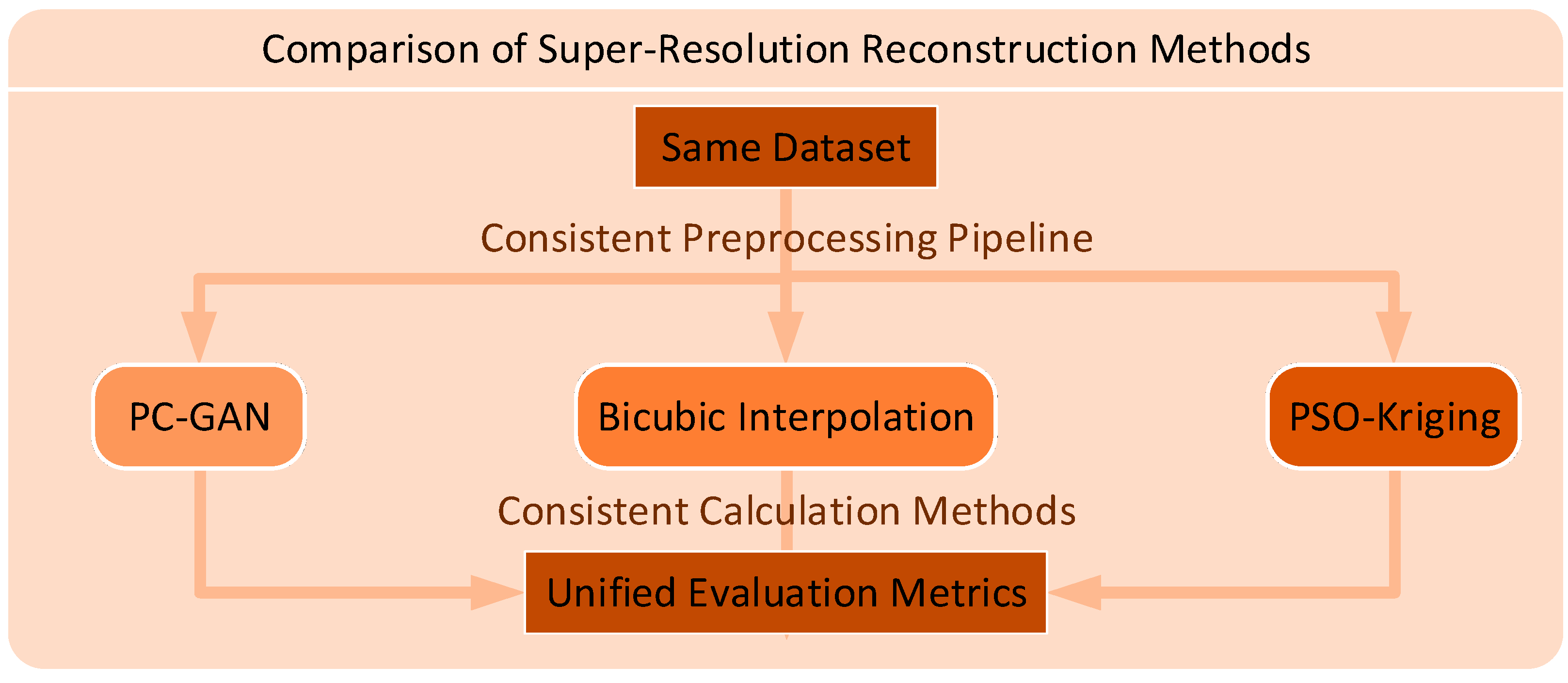
To rigorously benchmark the proposed PC-GAN, two reference algorithms were selected that, respectively, represent the state-of-the-art baselines in image super-resolution and in geophysical grid interpolation.

• Bicubic interpolation is the most widely adopted classic in the computer-vision community for single-image super-resolution; it is parameter-free, computationally lightweight, and universally treated as the lower-bound reference in deep learning studies [26].
• PSO-Kriging is the most recent variant of the standard Kriging family used in geomagnetic data processing. Traditional Kriging already serves as the geophysical baseline for sparse-grid interpolation, yet its semivariogram parameters are usually hand-tuned. By embedding particle-swarm optimization, PSO-Kriging automatically determines these parameters and has been shown to outperform ordinary Kriging, thus providing a stronger geophysical benchmark while remaining a non-deep learning approach [27].

Consequently, the pairing of bicubic interpolation and PSO-Kriging offers a balanced comparison: the former tests general image-reconstruction quality, whereas the latter tests adherence to geophysical spatial-statistics assumptions. Additional deep learning competitors (e.g., SRCNN or ESRGAN) were intentionally excluded because the present work itself is a generative-adversarial enhancement; contrasting against other neural architectures would shift the focus away from the central question of whether the newly introduced physics-informed constraints improve upon the generic SRGAN backbone. The experimental workflow is illustrated in Figure 5.

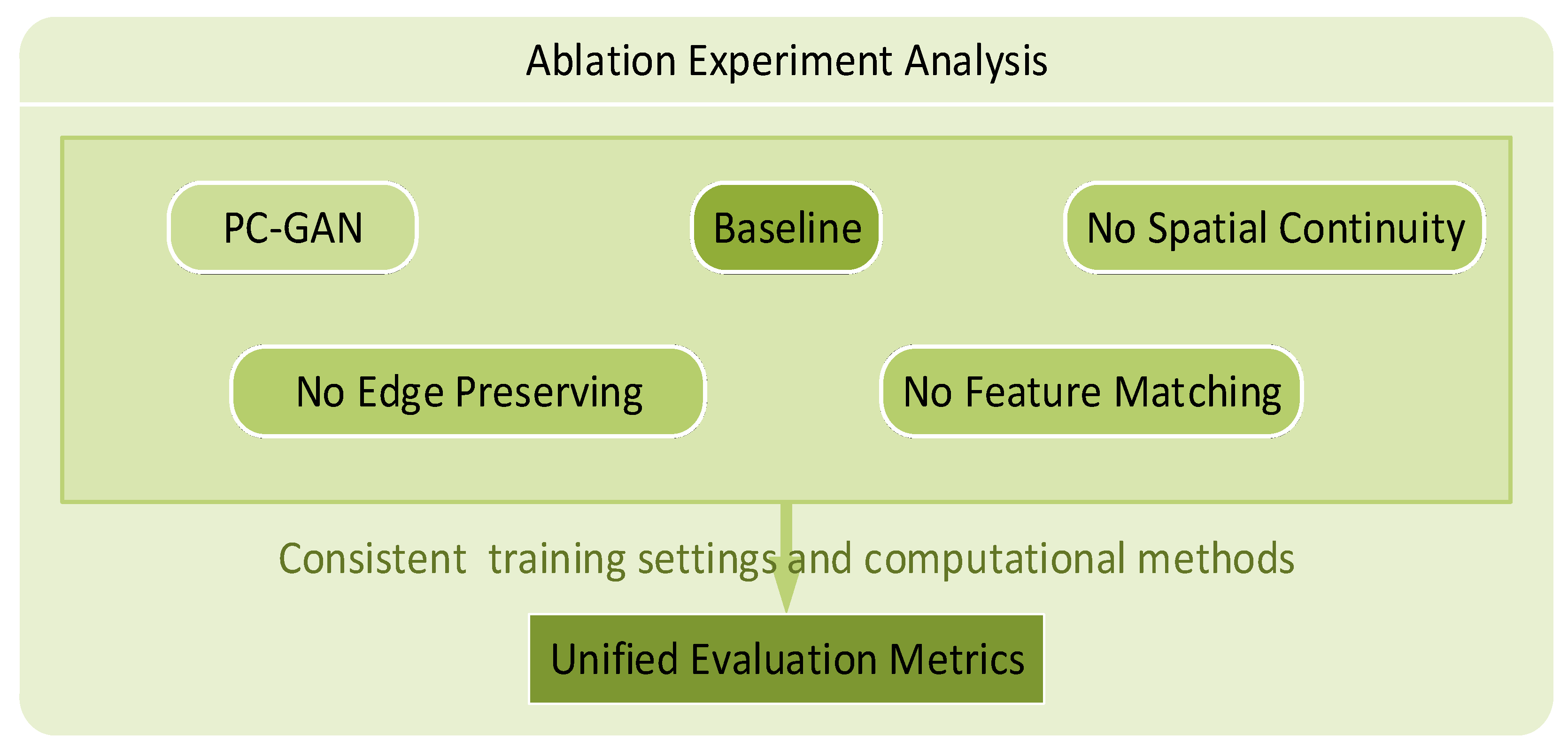
Additionally, five ablation studies were devised to quantify the individual contributions and combined influence of the PC GAN model’s three core loss terms, namely feature matching, spatial continuity and edge preservation, on the super resolution accuracy of geomagnetic anomaly reference maps. Using a baseline model as the control, the functional value of each component was quantified by removing one additional loss term or constraint module at a time. Experiments were conducted on samples from four typical sea areas in the EMAG2_V3 dataset, with RMSE, MAE, PSNR, and SSIM consistently adopted as evaluation metrics to ensure result fairness and comparability. The ablation experiment workflow is illustrated in Figure 6.

4. Results and Discussions

The entire workflow of experimental design has been completed in this chapter, covering data preprocessing, training configuration, and the determination of comparative methods as well as evaluation metrics. This provides a solid foundation for the generation of experimental results. The next chapter will conduct a systematic analysis of the experimental results. First, the performance differences between PC-GAN and traditional methods across the four marine regions will be compared using quantitative metrics. Then, the reconstruction effects will be intuitively presented by combining visualization results and residual analysis. Meanwhile, the role of each loss module will be verified through the results of ablation experiments. Finally, an in-depth discussion will be carried out on the advantages and applicable scenarios of PC-GAN in the super-resolution reconstruction of marine geomagnetic data.

4.1. Comparative Experimental Results

4.1.1. Quantitative Analysis of Numerical Metrics

To validate the superiority of PC-GAN in super-resolution reconstruction of marine geomagnetic anomaly reference maps, PSO-Kriging interpolation and bicubic interpolation were selected as comparative methods. Data were randomly selected from test sets constructed for four regions: the Philippine Sea Plate, East Pacific Rise, Northwest Pacific Ocean, and South Mid-Atlantic Ridge. Quantitative comparisons were conducted across two dimensions: numerical error and reconstruction quality. Experimental data for all methods were based on the same 32 × 32 low-resolution inputs and 64 × 64 high-resolution references, ensuring comparison fairness. Detailed results are presented in

Table 1. Performance of PC-GAN in Super-Resolution Reconstruction of Geomagnetic Anomaly Grid Data in the Philippine Sea Plate.

Algorithm	RMSE	MAE	PSNR	SSIM
Bicubic	1.222	0.795	33.700	0.947
PSO-Kriging	1.214	0.801	33.756	0.947
PC-GAN	0.880	0.611	36.550	0.976

,

Table 2. Performance of PC-GAN in Super-Resolution Reconstruction of Geomagnetic Anomaly Grid Data in the East Pacific Rise.

Algorithm	RMSE	MAE	PSNR	SSIM
Bicubic	1.380	0.921	34.633	0.940
PSO-Kriging	1.391	0.926	34.562	0.940
PC-GAN	1.057	0.806	36.951	0.945

,

Table 3. Performance of PC-GAN in Super-Resolution Reconstruction of Geomagnetic Anomaly Grid Data in the Northwest Pacific Ocean.

Algorithm	RMSE	MAE	PSNR	SSIM
Bicubic	1.212	0.880	36.857	0.960
PSO-Kriging	1.220	0.888	36.800	0.960
PC-GAN	1.125	0.897	37.502	0.963

and

Table 4. Performance of PC-GAN in Super-Resolution Reconstruction of Geomagnetic Anomaly Grid Data in the South Mid-Atlantic Ridge.

Algorithm	RMSE	MAE	PSNR	SSIM
Bicubic	1.481	1.033	34.415	0.934
PSO-Kriging	1.490	1.039	34.363	0.934
PC-GAN	1.197	0.915	36.260	0.945

. To quantify model stability, we trained the model five times from scratch while keeping the data split fixed. Across all four basins, RMSE, PSNR and SSIM exhibit small inter-run variability: RMSE standard deviation is no greater than 0.02 nT, PSNR standard deviation does not exceed 0.05 dB, and SSIM standard deviation remains below 0.001, indicating that PC-GAN produces consistently superior results.

As shown in Table 1, Table 2, Table 3 and Table 4, in the four regions with different geomagnetic characteristics, the super-resolution results of PC-GAN are significantly better than those of bicubic interpolation and PSO-Kriging interpolation in most quantitative indicators.

From the perspective of regional indicators, the Philippine Sea Plate shows the largest optimization margin for PC-GAN. Relative to bicubic and PSO-Kriging interpolation, the proposed method lowers RMSE by 28.0% and 27.5%, MAE by 23.1% and 23.6%, and simultaneously raises PSNR and SSIM, demonstrating a significant gain in structural similarity. In the East Pacific Rise, PC-GAN reduces RMSE by 23.4% and 23.9% (vs. the two methods), MAE by 12.5% and 13.0%, and PSNR/SSIM increases are smaller than in the Philippine Sea Plate. In the Northwest Pacific Ocean, PC-GAN’s RMSE reduction vs. the two methods is relatively small; MAE fluctuates but has a more uniform overall error distribution (no obvious trend), and PSNR/SSIM optimization margins are limited. In the South Mid-Atlantic Ridge, PC-GAN still maintains a significant RMSE reduction vs. the two methods, with stable optimization margins for MAE and PSNR, and a certain SSIM improvement.

From a principled perspective: Bicubic interpolation relies solely on nonlinear weighted fitting of pixel neighborhoods and lacks task-specific adaptation mechanisms. In scenarios with low adaptability requirements, its error gap with PC-GAN is small (due to low data fitting difficulty); as adaptability requirements rise, its over-smoothing leads to rapid error accumulation, and performance disadvantages become prominent. Although PSO-Kriging captures spatial dependence by using particle-swarm optimization to fit the semivariogram, its reliance on a single global variogram model limits local adaptability, and the resulting residuals grow in proportion to the heterogeneity of the target scene. By contrast, PC-GAN builds a comprehensive adaptation mechanism via a multi-objective loss function: content loss (centered on RMSE) ensures basic numerical accuracy, spatial continuity loss suppresses local unreasonable deviations, and edge preservation loss optimizes detailed feature restoration. This allows PC-GAN to targetedly meet different scenarios’ adaptability needs. Consequently, as adaptability demands intensify, the architectural advantages of PC-GAN are fully mobilized: it secures superior performance in every region, and the margin of optimization widens in direct proportion to the severity of the adaptation challenge.

4.1.2. Visual Comparison and Residual Analysis

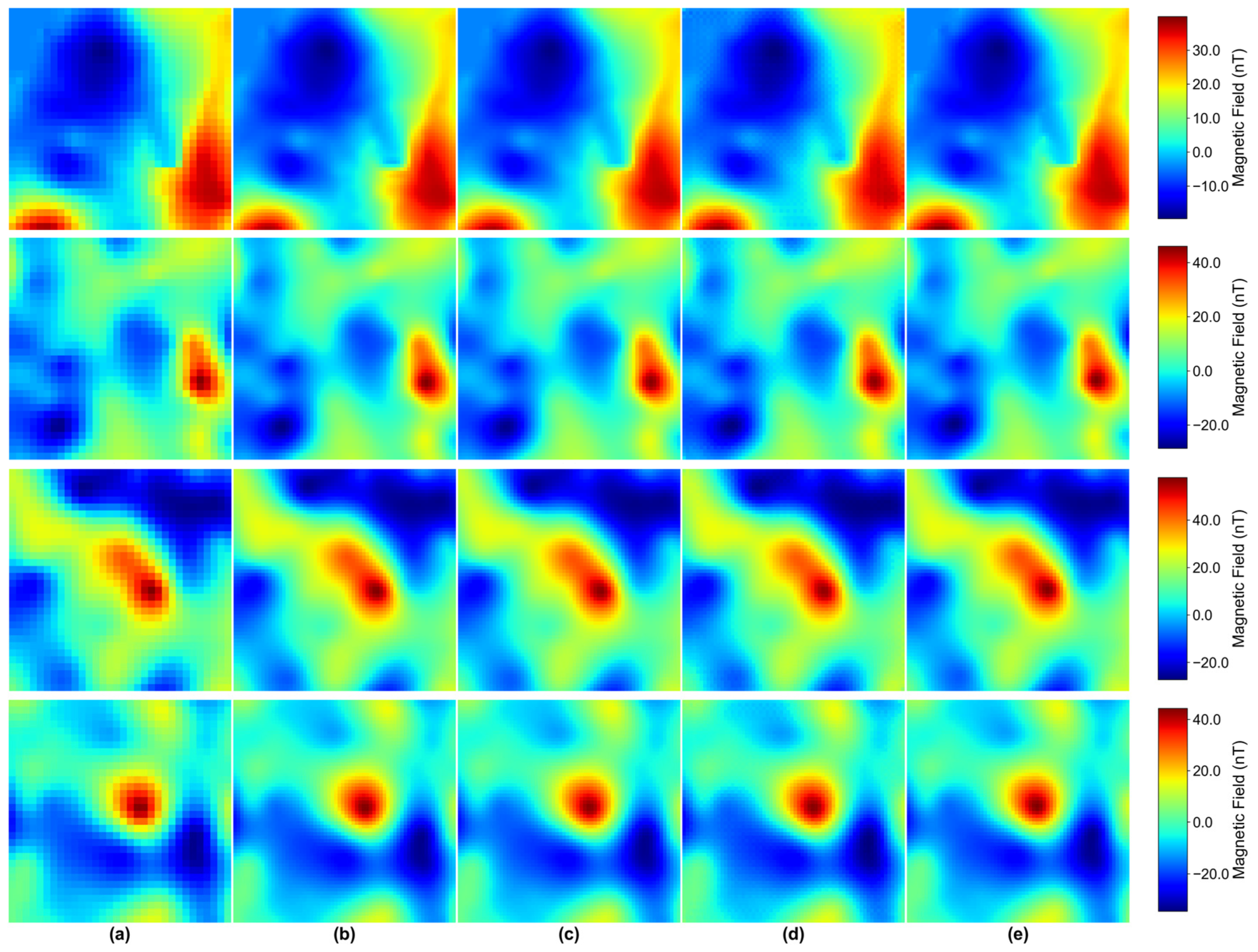
To intuitively validate the fidelity of geomagnetic anomaly details and spatial continuity of the proposed method, Figure 7 presents visual comparison results of all methods across the four regions. Specifically, Figure 7a shows 32 × 32 low-resolution input data; Figure 7b–d display 64 × 64 reconstruction results from bicubic interpolation, PSO-Kriging, and the proposed method, respectively; and Figure 7e provides the 64 × 64 real high-resolution reference data.

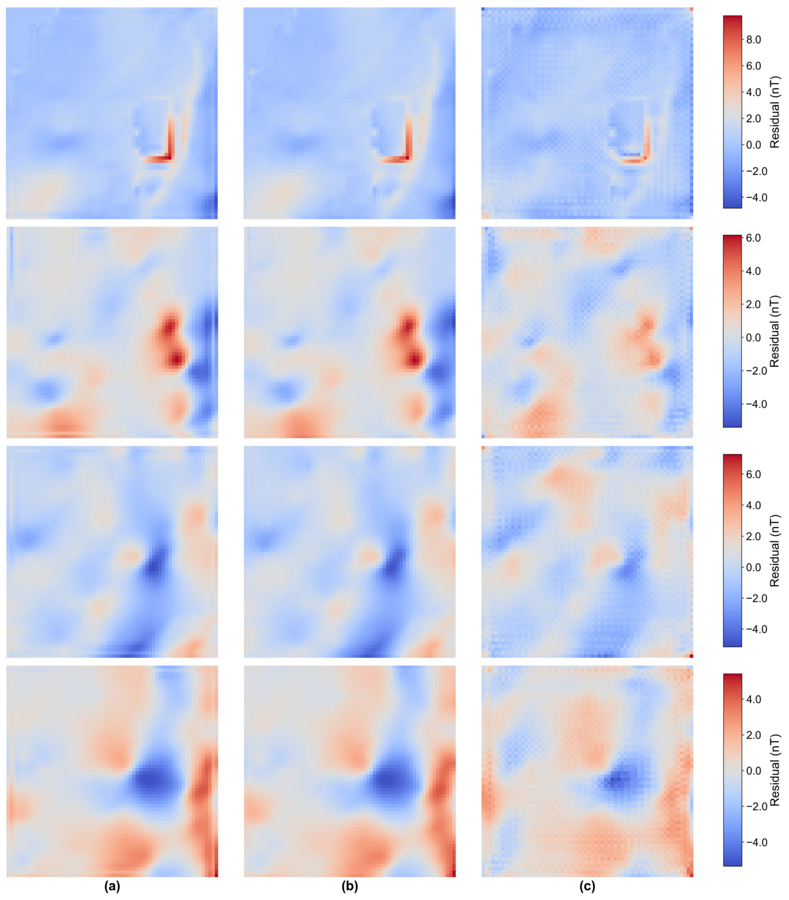
From the perspective of macro visual presentation, the reconstruction results of the three methods do not show extremely strong intuitive differences. Figure 8 shows the reconstruction residual comparison results of each method. Figure 8a–c are the residual maps of bicubic interpolation, PSO-Kriging, and the proposed method, respectively. The dark-colored areas in the residual map of bicubic interpolation are significantly more than those in the other two methods, with a wide error distribution. Especially in areas where geomagnetic anomalies change drastically, the color depth increases significantly, indicating that the errors in these detailed areas are significantly higher than those in other areas. Although the residual map of PSO-Kriging has fewer dark-colored areas than that of bicubic interpolation, there are still obvious dark red areas in places where the geomagnetic anomaly gradient changes sharply, indicating that the error control for local details is still insufficient. The residual map of the proposed method in this paper has a more uniform overall color, with errors distributed only in very few areas. The dark-colored high-error areas are significantly fewer, and the error distribution is more uniform. Even in areas with rich geomagnetic anomaly details, the error at error points is smaller and the color is more uniform. This result proves that the proposed method has better error control capability, and can achieve a balance between macro-feature restoration and detailed error suppression, further verifying its comprehensive advantages in numerical accuracy and physical rationality in geomagnetic anomaly super-resolution reconstruction.

4.2. Ablation Experiment Results

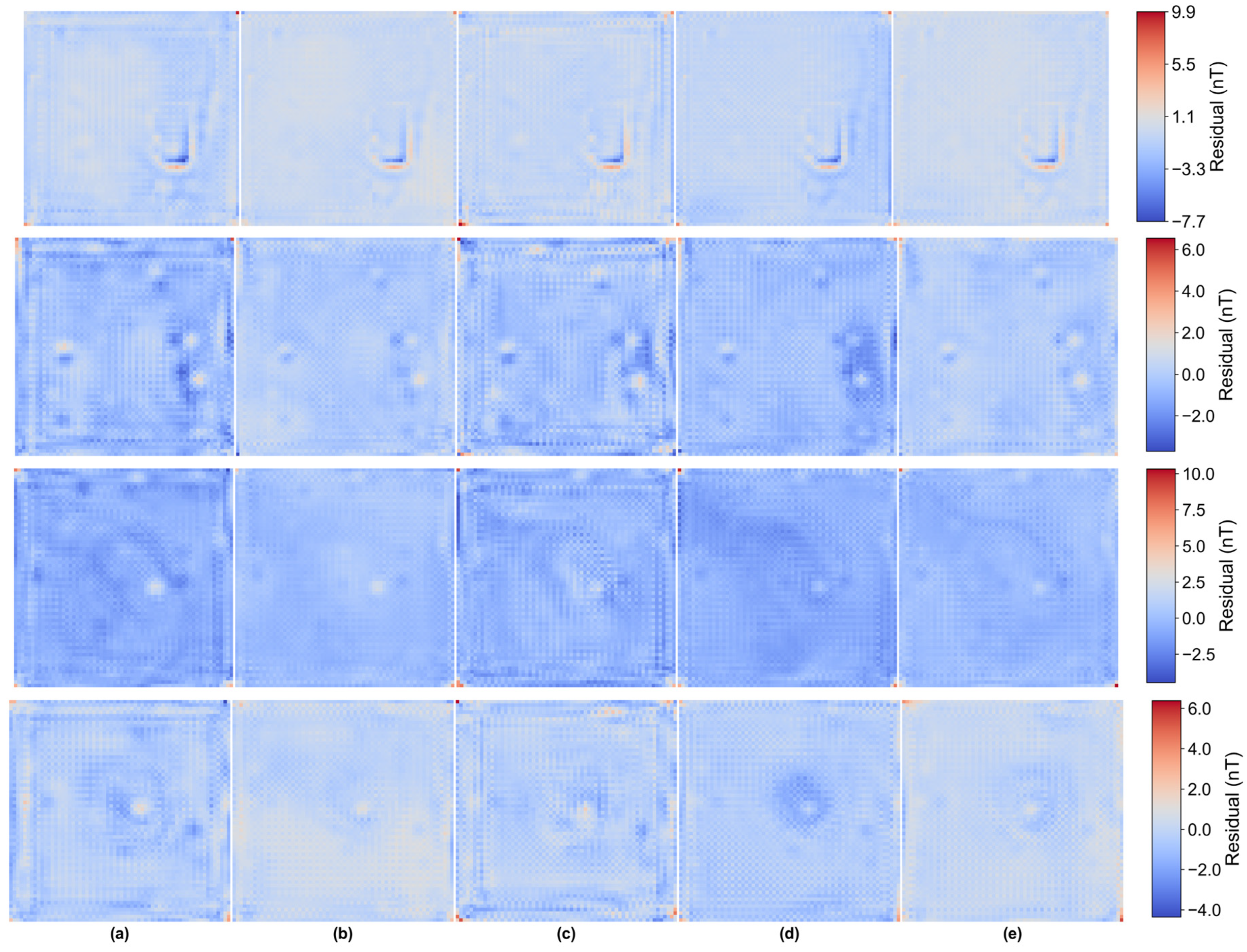
To quantify how each loss term in PC-GAN affects super-resolution accuracy, we first established a baseline model. Five ablation experiments were then conducted. These experiments isolate and combine the feature-matching, spatial-continuity and edge-preservation losses, allowing their individual contributions and joint effect on geomagnetic-anomaly reference maps to be compared with the full PC-GAN model. All experiments were conducted on four typical sea area samples from the EMAG2_V3 dataset, with consistent use of evaluation metrics: RMSE, MAE, PSNR, and SSIM to ensure result fairness and comparability. To intuitively reflect the error distribution differences between the ablation groups and the full PC-GAN model, residual maps of the super-resolution results for the four marine regions under different experimental settings are displayed in Figure 9. Specific quantitative results are presented in

Table 5. Super-resolution Reconstruction Performance of the Ablation Experiment Training Set.

Algorithm	RMSE	MAE	PSNR	SSIM
No Edge Preservation Loss	2.055	1.404	41.237	0.987
No Feature-Matching Loss	1.913	1.326	41.898	0.987
No Spatial Continuity Loss	1.510	0.967	44.795	0.995
Baseline	2.057	1.508	41.070	0.981
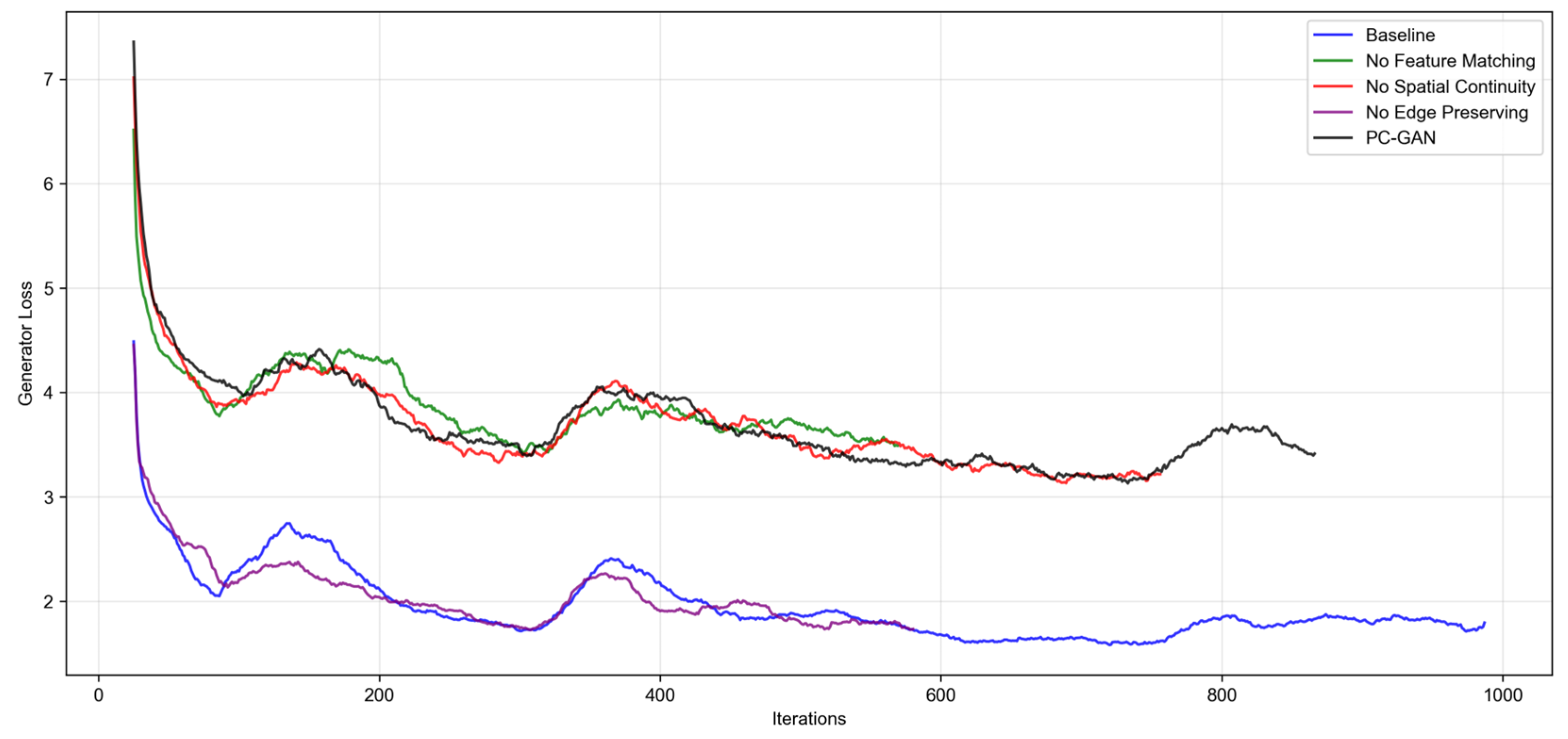
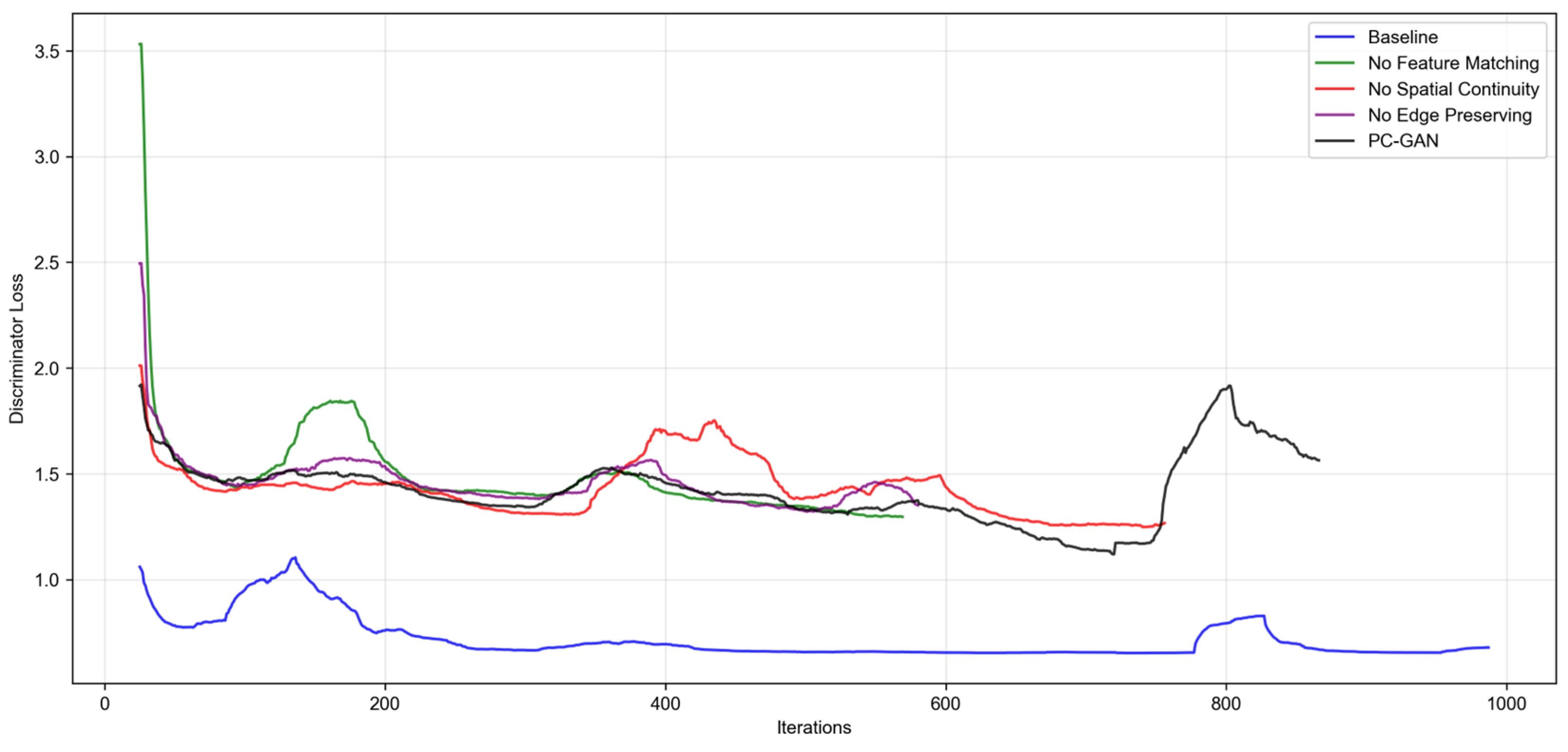
PC-GAN	1.414	0.964	44.908	0.995

, while generator and discriminator loss curves during training are shown in Figure 10 and Figure 11. All metrics are reported as mean ± standard deviation over five runs.

As indicated in Table 5, the full PC-GAN model outperforms all ablation groups and the baseline model in comprehensive performance. Omitting any core module degrades performance, and each module’s function aligns with the requirements of geomagnetic anomaly reconstruction: the baseline model exhibits the poorest metrics. By integrating the four modules, the full PC-GAN achieves a 31.26% reduction in RMSE, a 36.07% reduction in MAE, a 3.838 dB increase in PSNR, and an SSIM improvement to 0.995. This confirms that a single loss cannot fully meet the requirements, and synergistic interaction between modules is essential.

The baseline model’s generator loss decreases most rapidly: it drops to approximately 2 after 200 iterations, maintains stability, and finally stabilizes at around 1.8. This is attributed to its loss function, which features low complexity and fast convergence. However, the lack of refined constraints limits further improvement in the generator’s ability to learn geomagnetic anomaly details. The loss curves of the “without feature matching loss” and “without spatial continuity loss” groups show similar trends: they stabilize between 3.5 and 4.5 after 100–300 iterations, with both convergence speed and final loss values inferior to the full PC-GAN model. The full PC-GAN model’s generator loss decreases rapidly after 100 iterations, enters a stable convergence phase after 200 iterations, and finally stabilizes at approximately 3.2. This validates the synergistic effect of the three core modules: they not only ensure the generator’s learning efficiency but also prevent premature convergence caused by an overly simple loss function through refined constraints, thereby effectively enhancing model performance.

The baseline model’s discriminator loss decreases most rapidly and stably: it falls below 1 within 100 iterations and finally stabilizes at around 0.5. This is because its loss function only requires the discriminator to simply distinguish between generated and real data, resulting in a single learning objective and extremely fast convergence. However, this also leads to insufficient ability of the discriminator to judge the rationality of geomagnetic data, preventing it from providing accurate supervision for the generator. The discriminator losses of the “without feature matching,” “without spatial continuity,” and “without edge preservation” groups remain in the 1.5–2.5 range for an extended period with significant fluctuations: the “without feature matching” group rebounds after an initial decline, while the “without spatial continuity” and “without edge preservation” groups exhibit continuous oscillations. This is because feature matching, spatial continuity, and edge preservation losses require the discriminator to more rigorously verify whether generated data complies with geomagnetic physical laws, increasing learning complexity and thus causing slower convergence and larger loss fluctuations. The discriminator loss of the full PC-GAN model declines gradually after the 100th iteration and stabilizes between 1.2 and 1.8 for an extended period; the minor rise observed around iteration 800 coincides with the discriminator’s retraining in response to the generator’s advancement. This indicates that under the synergy of the four core modules, the discriminator must simultaneously perform two tasks: distinguishing between real and fake data, and supervising geomagnetic physical features. This more complex learning task results in higher loss than the baseline; however, this in-depth supervision provides more accurate feedback to the generator, which is the key to the model’s superior performance.

5. Conclusions

This study introduces PC-GAN as a new route toward enhancing the precision of marine geomagnetic reference maps and provides technical support for high-accuracy geomagnetic matching navigation. The main contributions are threefold:

• We redesign the SRGAN loss function by incorporating three terms: spatial continuity, edge preservation, and perceptual feature matching. This physics-informed combination yields a measurable accuracy gain.
• Comparative and ablation experiments demonstrate that PC-GAN outperforms both traditional methods and the original SRGAN, reducing RMSE by up to 28% and increasing PSNR by approximately 2.8 dB.

The present approach is still constrained by its two-dimensional assumption: the network operates only on surface grids and does not exploit along-track depth or airborne elevation information, so fine-scale recovery may be incomplete in complex 3-D geological settings. Moreover, the current inference time of about 0.13 s per 1° × 1° block may not meet real-time demands in field applications; further compression of both the computational graph and memory footprint is therefore required before deployment on embedded GPUs.

Future research will pursue two directions. First, the framework will be extended to three-dimensional data by introducing depth-aware constraints to enable true 3-D geomagnetic map reconstruction. Second, the model will be optimized and fused with multi-source data to improve computational efficiency and robustness, allowing the super-resolution module to update reference maps online during shipborne or AUV operations.