A Boundary-Implicit Constraint Reconstruction Method for Solving the Shallow Water Equations

Abstract

To improve the accuracy of second-order cell-centered finite volume method in near-boundary regions for solving the two-dimensional shallow water equations, a numerical scheme with globally second-order accuracy was proposed. Having the primary objective to overcome the challenge of accuracy degradation in near-boundary regions and to develop a robust numerical framework combining high-order accuracy with strict conservation, the key research objectives had been as follows: Firstly, a physical variable reconstruction method combining a vertex-based nonlinear weighted reconstruction scheme and a monotonic upwind total variation diminishing scheme for conservation laws was proposed. While the overall computational efficiency was maintained, linear-exact reconstruction in near-boundary regions was achieved. The variable reconstruction in interior regions was integrated to achieve global second-order accuracy. Subsequently, a flux boundary condition treatment method based on uniform flow was proposed. Conservative allocation of hydraulic parameters was achieved, and flow stability in inflow regions was enhanced. Finally, a series of numerical test cases were provided to validate the performance of the proposed method in solving the shallow water equations in terms of high-order accuracy, exact conservation properties, and shock-capturing capabilities. The superiority of the method was further demonstrated under high-speed flow conditions. The high-precision numerical model developed in this study holds significant value for enhancing the predictive capability of simulations for natural disasters such as flood propagation and tsunami warning. Its robust boundary treatment methods also provide a reliable tool for simulating free-surface flows in complex environments, offering broad prospects for engineering applications.

1. Introduction

The second-order Godunov-type cell-centered finite volume method (FVM) which has efficiency, stability, and accuracy advantages in dealing with complex flow field problems was widely used for solving shallow water equations (SWEs) in hydraulics, oceanography, and environmental engineering [1,2,3,4]. Physical variable reconstruction was identified as the critical step to ensure global accuracy in the finite volume method [5]. Gradient reconstruction methods for unstructured grids were mainly classified into two categories: the Green–Gauss (GG) method [6,7] and the weighted least squares (WLSQ) method [8,9]. For the numerical solution of shallow water equations, the monotonic upstream-centered scheme for conservation laws (MUSCL) reconstruction method based on the piecewise linear assumption was established as the mainstream approach. MUSCL reconstruction was employed by performing linear reconstruction of conserved quantities within cells and integrating limiter techniques to suppress numerical oscillations, thereby maintaining high resolution while avoiding non-physical phenomena [10,11]. Hou et al. [10], Song et al. [12], and Yu et al. [13] have all employed the MUSCL approach to develop two-dimensional well-balanced shallow water flow models based on unstructured cell-centered finite volume methods. However, in their implementations, if a boundary cell has one edge on the boundary, the gradient has been computed using the cell centroid and two adjacent centroids within the computational domain. For boundary cells with two edges on the boundary, the boundary variable values have simply been set equal to the cell-centered values. Furthermore, the variable values on boundary faces have been constructed using a first-order extrapolation from the boundary cell centroid values [10,11]. Therefore, a reduction in the model’s accuracy has been observed in near-boundary regions.

Only limited research was specifically focused on the performance of gradient reconstruction algorithms in near-boundary regions [9,14,15,16]. Inaccurate boundary variable reconstruction leads to at least first-order accuracy loss in boundary regions compared to interior domains [17]. Zhang et al. proposed a novel vertex-based solution reconstruction method [18]. The vertex-based weighted least squares (VWLSQ) procedure was first employed, and cell-centered solutions were utilized to calculate the gradients at mesh vertices. Chen et al. proposed a grid-based partially implicit weighted least squares method (BIVWLSQ) [9]. This method enhanced the accuracy and efficiency of numerical simulations through an innovative reconstruction strategy. It has been successfully applied to transient wave problems and the solution of Euler equations [14,15,19,20]. BIVWLSQ demonstrated high efficiency and robustness in handling complex flow problems, particularly excelling in capturing shocks and discontinuities in these applications.

To accurately capture shock waves and ensure the robustness of numerical simulations, high-performance slope limiters were typically required [18,21]. Some commonly used slope limiters failed to strictly guarantee the monotonicity principle [22]. Therefore, nonlinear weighting strategies were extensively employed in spatial reconstruction on unstructured grids, in addition to traditional slope limiting strategies [23]. These high-order methods based on nonlinear weighting strategies primarily followed the weighted essentially non-oscillatory (WENO) scheme [24]. Numerical oscillations near discontinuities were effectively suppressed by dynamically adjusting weights and combining smoothness indicators from multiple sub-stencils, while high accuracy and resolution were preserved in smooth regions [9,15,23].

The treatment of boundary conditions was a critical component in two-dimensional shallow water flow simulations [25,26]. Two primary approaches have been implemented for enforcing boundary conditions in mathematical models: the ghost cell method [25] and the direct numerical flux computation method [10,11,12,26]. The inflow hydrograph was typically prescribed; however, the rational allocation of hydraulic parameters at the inflow boundary based on cross-sectional discharge became a key research focus for most flood propagation simulations. The Manning and Chezy formulas have been utilized by Song et al. [12] to calculate weights based on water depth and grid edge length at boundaries for discharge allocation. A uniform flow approach has been adopted by Hou et al. [25] on inflow boundary grids by determining the longitudinal slope of the channel, through which water levels have been determined and hydraulic parameters across boundary grids have been allocated.

Globally second-order accurate schemes have not been thoroughly investigated for the accuracy of the second-order cell-centered finite volume method in solving two-dimensional shallow water equations in near-boundary regions. A global second-order method that enhances near-boundary accuracy has been proposed in this study based on the existing framework [9,12,13]. First, hyperbolic partial differential equations are employed to create a mesh using triangular cells of arbitrary geometry. Second, a monotonic upstream-centered scheme for conservation laws with MUSCL-TVD is adopted for physical variable reconstruction in interior regions, while BIVWLSQ reconstruction scheme is applied in near-boundary regions. This approach maintains overall computational efficiency while achieving linear-exact reconstruction near boundaries. Subsequently, the Harten–Lax–van Leer-Contact (HLLC) approximate Riemann solver is selected to compute fluxes at cell interfaces. Finally, a flux boundary condition treatment method based on uniform flow theory is designed, which significantly enhances flow stability in inflow regions through conservative allocation of hydraulic parameters. A series of numerical test cases validate the proposed model, with results compared against existing experimental data.

2. Governing Equations and Numerical Methods

2.1. Modified Shallow Water Equations

The standard two-dimensional shallow water equations are as follows:

$${\displaystyle \frac{\mathsf{\partial }U}{\mathsf{\partial }t}}+{\displaystyle \frac{\mathsf{\partial }E}{\mathsf{\partial }x}}+{\displaystyle \frac{\mathsf{\partial }G}{\mathsf{\partial }y}}=S$$

(1)

where $U$ is the vector of conservative variables; $E$ and $G$ are the convective fluxes in the x- and y-directions, respectively; $t$ is the temporal variable; $x$ and $y$ are the spatial coordinates; and $S$ is the source term.

$$\begin{gathered} U=\left[\begin{array}{c}h\\ hu\\ hv\end{array}\right],E=\left[\begin{array}{c}hu\\ h{u}^2+g{h}^2/2\\ huv\end{array}\right],G=\left[\begin{array}{c}hv\\ huv\\ h{v}^2+g{h}^2/2\end{array}\right], \\ S=S_b+S_f=\left[\begin{array}{c}0\\ -gh\mathsf{\partial }b/\mathsf{\partial }x\\ -gh\mathsf{\partial }b/\mathsf{\partial }y\end{array}\right]+\left[\begin{array}{c}0\\ -gh{\displaystyle \frac{n^{2}u\sqrt{u^2+v^2}}{h^{4/3}}}\\ -gh{\displaystyle \frac{n^{2}v\sqrt{u^2+v^2}}{h^{4/3}}}\end{array}\right]. \end{gathered}$$

(2)

where $h$ is the water depth; $u$ and $v$ are the flow velocities in the x- and y-directions, respectively; $g$ is the gravitational acceleration; $S_b$ and $S_f$ are the bed slope source term and friction source term, respectively; and $n$ is the Manning’s roughness coefficient.

In this work, sloped-bottom triangular cell grids and a cell-centered bed slope term calculation method are adopted. To avoid calculating correction terms, the modified form of the governing equations [12] is employed:

$${\displaystyle \frac{\mathsf{\partial }U}{\mathsf{\partial }t}}+{\displaystyle \frac{\mathsf{\partial }E}{\mathsf{\partial }x}}+{\displaystyle \frac{\mathsf{\partial }G}{\mathsf{\partial }y}}=S$$

(3)

$$\begin{gathered} U=\left[\begin{array}{c}h\\ hu\\ hv\end{array}\right],E=\left[\begin{array}{c}hu\\ h{u}^2+g\left(h^2-b^2\right)/2\\ huv\end{array}\right],G=\left[\begin{array}{c}hv\\ huv\\ h{v}^2+g\left(h^2-b^2\right)/2\end{array}\right], \\ S=S_b+S_f=\left[\begin{array}{c}0\\ -g\left(h+b\right)\mathsf{\partial }b/\mathsf{\partial }x\\ -g\left(h+b\right)\mathsf{\partial }b/\mathsf{\partial }y\end{array}\right]+\left[\begin{array}{c}0\\ -gh{\displaystyle \frac{n^{2}u\sqrt{u^2+v^2}}{h^{4/3}}}\\ -gh{\displaystyle \frac{n^{2}v\sqrt{u^2+v^2}}{h^{4/3}}}\end{array}\right]. \end{gathered}$$

(4)

where $b$ is the bottom elevation.

2.2. Time and Space Discretization for SWEs on Triangular Grids

Within an unstructured cell-centered triangular cell grid, the integral form of Equation (3) is expressed as

$$\underset{\Omega }{\int }{\displaystyle \frac{\mathsf{\partial }U}{\mathsf{\partial }t}}d\Omega +\underset{\Omega }{\int }{\displaystyle \frac{\mathsf{\partial }E}{\mathsf{\partial }x}}+{\displaystyle \frac{\mathsf{\partial }G}{\mathsf{\partial }y}}d\Omega =\underset{\Omega }{\int }Sd\Omega$$

(5)

where $\Omega$ is the control volume. By applying Green’s theorem to convert the area integral in Equation (5) into a line integral, the governing equation can be rewritten as

$$A_i{\displaystyle \frac{d{U}_i}{dt}}+{\displaystyle \sum _{k=1}^3}{F}_{i,k}{n}_{i,k}{l}_{i,k}=A_i{S}_i$$

(6)

where $A_i$ is the cell area; $i$ is the cell index; $n$ is the outward normal vector at the cell boundary; $k$ and $l$ are the edge index and length of cell $i$, respectively; and $F_{i,k}$ is the numerical flux, which can be obtained by solving the Riemann problem [27,28]. By employing a multi-stage Runge–Kutta scheme for temporal discretization of the time derivative terms in Equation (6) to achieve second-order temporal accuracy, the governing equation can be rewritten as

$$U^{n+1/2}=U^n+{\displaystyle \frac{∆t}{A_i}}{\left(-{\displaystyle \sum _{k=1}^3}{F}_{i,k}{n}_{i,k}{l}_{i,k}+A_i{S}_i\right)}_n$$

(7)

$$U^{n+1}={\displaystyle \frac{1}{2}}{U}^n+{\displaystyle \frac{1}{2}}{U}^{n+1/2}+{\displaystyle \frac{∆t}{{2A}_i}}{\left(-{\displaystyle \sum _{k=1}^3}{F}_{i,k}{n}_{i,k}{l}_{i,k}+A_i{S}_i\right)}_{n+1/2}$$

(8)

where $U^{n+1/2}$ is the intermediate variable.

2.3. MUSCL Reconstruction

To enhance the spatial accuracy of the scheme, higher-order reconstruction methods than piecewise-constant approximations must be adopted to reconstruct the left and right interface states when constructing local Riemann problems at cell interfaces. The numerical flux at the interface is then computed based on these reconstructed variables [10,11,17]. The reconstructed values of water depth and flow velocity at the interface are computed through linear reconstruction combined with a limiter function:

$$U_{i,k}=U_i^c+{\nabla }_i^{l}r$$

(9)

where $U_{i,k}$ is the reconstructed value at the $k$-th edge of cell $i$; $U_i^c$ is the variable value at the center of cell $i$; $r$ is the position vector from the cell center to the $k$-th edge center of cell $i$; and ${\nabla }_i^l$ is the limited gradient, defined as

$${\nabla }_i^l=\underset{k=\mathrm{1,2},3}{\mathit{min}}\left({\alpha }_k\right){\nabla }_i^{un}$$

(10)

where ${\nabla }_i^{un}$ is the unlimited gradient and ${\alpha }_k$ is the limiter function, which is computed as follows:

$${\alpha }_k=\left\{\begin{array}{cc}\mathit{min}\left[1,{\displaystyle \frac{\mathit{max}\left(0,U_{i,k}^{nc}-U_i^c\right)}{U_{i,k}^{un}-U_i^c}}\right]& if{U}_{i,k}^{un}-U_i^c>0\\ 1& if{U}_{i,k}^{un}-U_i^c=0\\ \mathit{min}\left[1,{\displaystyle \frac{\mathit{min}\left(0,U_{i,k}^{nc}-U_i^c\right)}{U_{i,k}^{un}-U_i^c}}\right]& if{U}_{i,k}^{un}-U_i^c<0\end{array}\right.$$

(11)

where $U_{i,k}^{nc}$ is the variable value at the center of the neighboring cell sharing the $k$-th edge with cell $i$.

2.4. BIVWLSQ Boundary Variable Reconstruction

The well-posedness of the Navier–Stokes equations fundamentally relies on initial-boundary value conditions, where errors in boundary values directly affect the accuracy of the entire flow field. Therefore, the simultaneous acquisition of second-order accurate variable values within cells and at boundary face elements is critical to ensuring globally consistent second-order accuracy in the finite volume method [9,18]. In this work, an implicit near-boundary gradient reconstruction method is employed, in which boundary constraints are fully considered during the gradient reconstruction process. The gradient calculation and boundary value computation are integrated into a unified system for solving. This implicit strategy is further combined with the explicit vertex-based weighted least squares method. For gradient computation at mesh vertices, adjacent cells are utilized as stencils, as illustrated in Figure 1.

Assuming $a$ vertex is the target for gradient reconstruction, the cell-centered variables of its adjacent cells are expressed based on the Taylor expansion formula as follows:

$$f_{i }=f_a+\nabla f_a∆r_{ai}+h.o.t\approx f_a+{\displaystyle \frac{\mathsf{\partial }{f}_a}{\mathsf{\partial }x}}∆x_{ai}+{\displaystyle \frac{\mathsf{\partial }{f}_a}{\mathsf{\partial }y}}∆y_{ai}$$

(12)

where $f_{i }$ is the cell-centered variable value; $f_a$ is the vertex-centered variable value at vertex $a$; $\nabla f_a=\left({\displaystyle \frac{\mathsf{\partial }{f}_a}{\mathsf{\partial }x}},{\displaystyle \frac{\mathsf{\partial }{f}_a}{\mathsf{\partial }y}}\right)$ is the gradient at vertex $a$; $∆r_{ai}={\left(∆x_{ai},∆y_{ai}\right)}^T$ is the position vector from vertex $a$ to the centroid of adjacent cell $i$. If vertex $b$ is located on the boundary, additional gradient stencils are supplemented to provide sufficient information for gradient reconstruction. The strategy of using ghost cells as supplementary stencils is abandoned, and boundary face elements containing the target vertex are incorporated into the gradient stencils:

$$f_{bi }=f_b+\nabla f_b∆r_{bbi}+h.o.t\approx f_b+{\displaystyle \frac{\mathsf{\partial }{f}_b}{\mathsf{\partial }x}}∆x_{bbi}+{\displaystyle \frac{\mathsf{\partial }{f}_b}{\mathsf{\partial }y}}∆y_{bbi}$$

(13)

where $f_b$ is the cell-centered variable value; $f_{bi }$ is the boundary face-centered variable value; $\nabla f_b=\left({\displaystyle \frac{\mathsf{\partial }{f}_b}{\mathsf{\partial }x}},{\displaystyle \frac{\mathsf{\partial }{f}_b}{\mathsf{\partial }y}}\right)$ is the gradient at vertex $b$; and $∆r_{bbi}={\left(∆x_{bbi},∆y_{bbi}\right)}^T$ is the position vector from vertex $b$ to the centroid of its adjacent boundary face.

For the cell-centered finite volume method on unstructured grids, the WLSQ is employed to solve the unknown grid variables $f_a$, $f_b$, $\nabla f_a$, and $\nabla f_b$. The weighted sum of squared higher-order residuals from all stencils is obtained:

$$\begin{array}{cc}\hfill f\left(f_b,{\displaystyle \frac{\mathsf{\partial }{f}_b}{\mathsf{\partial }x}},{\displaystyle \frac{\mathsf{\partial }{f}_b}{\mathsf{\partial }y}}\right)=& {\displaystyle \sum _{i=1}^{N_i}}{\omega }_i{\left(f_i-f_b-{\displaystyle \frac{\mathsf{\partial }{f}_b}{\mathsf{\partial }x}}∆x_{bi}-{\displaystyle \frac{\mathsf{\partial }{f}_b}{\mathsf{\partial }y}}∆y_{bi}\right)}^2\hfill \\ & +{\displaystyle \sum _{i=1}^{N_{bi}}}{\omega }_{bi}{\left(f_{bi}-f_b-{\displaystyle \frac{\mathsf{\partial }{f}_b}{\mathsf{\partial }x}}∆x_{bbi}-{\displaystyle \frac{\mathsf{\partial }{f}_b}{\mathsf{\partial }y}}∆y_{bbi}\right)}^2\hfill \end{array}$$

(14)

where $N_i$ and $N_{bi}$ are the total numbers of cells and boundary face elements adjacent to the target vertex $b$, respectively; ${\omega }_i$ and ${\omega }_{bi}$ are the weights for the corresponding cells and boundary face elements, calculated as follows:

$${\omega }_{i\left(bi\right)}={\displaystyle \frac{1}{{L_{bi\left(bbi\right)}}^n}}$$

(15)

where $L_{bi}$ and $L_{bbi}$ are the distances from vertex $b$ to the adjacent cell and boundary face element, respectively; $n$ is the exponent. When $n=0$, it is equivalent to solving an unweighted least squares problem.

To obtain the optimal solution for the unknowns by minimizing the higher-order residual terms in Equation (14), the following equations are derived:

$$\begin{array}{cc}\hfill {\displaystyle \frac{\mathsf{\partial }f}{\mathsf{\partial }{f}_b}}=-{\displaystyle \sum _{i=1}^{N_i}}{2\omega }_i& \left(f_i-f_b-{\displaystyle \frac{\mathsf{\partial }{f}_b}{\mathsf{\partial }x}}∆x_{bi}-{\displaystyle \frac{\mathsf{\partial }{f}_b}{\mathsf{\partial }y}}∆y_{bi}\right)\hfill \\ & -{\displaystyle \sum _{i=1}^{N_{bi}}}2{\omega }_{bi}\left(f_{bi}-f_b-{\displaystyle \frac{\mathsf{\partial }{f}_b}{\mathsf{\partial }x}}∆x_{bbi}-{\displaystyle \frac{\mathsf{\partial }{f}_b}{\mathsf{\partial }y}}∆y_{bbi}\right)\hfill \\ \hfill {\displaystyle \frac{\mathsf{\partial }f}{\mathsf{\partial }\frac{\mathsf{\partial }{f}_b}{\mathsf{\partial }x}}}=-{\displaystyle \sum _{i=1}^{N_i}}{2\omega }_i& \left(f_i-f_b-{\displaystyle \frac{\mathsf{\partial }{f}_b}{\mathsf{\partial }x}}∆x_{bi}-{\displaystyle \frac{\mathsf{\partial }{f}_b}{\mathsf{\partial }y}}∆y_{bi}\right)∆x_{bi}\hfill \\ & -{\displaystyle \sum _{i=1}^{N_{bi}}}2{\omega }_{bi}\left(f_{bi}-f_b-{\displaystyle \frac{\mathsf{\partial }{f}_b}{\mathsf{\partial }x}}∆x_{bbi}-{\displaystyle \frac{\mathsf{\partial }{f}_b}{\mathsf{\partial }y}}∆y_{bbi}\right)∆x_{bbi}\hfill \\ \hfill {\displaystyle \frac{\mathsf{\partial }f}{\mathsf{\partial }\frac{\mathsf{\partial }{f}_b}{\mathsf{\partial }y}}}=-{\displaystyle \sum _{i=1}^{N_i}}{2\omega }_i& (f_i-f_b-{\displaystyle \frac{\mathsf{\partial }{f}_b}{\mathsf{\partial }x}}∆x_{bi}-{\displaystyle \frac{\mathsf{\partial }{f}_b}{\mathsf{\partial }y}}∆y_{bi})∆y_{bi}\hfill \\ & -{\displaystyle \sum _{i=1}^{N_{bi}}}2{\omega }_{bi}(f_{bi}-f_b-{\displaystyle \frac{\mathsf{\partial }{f}_b}{\mathsf{\partial }x}}∆x_{bbi}-{\displaystyle \frac{\mathsf{\partial }{f}_b}{\mathsf{\partial }y}}∆y_{bbi})∆y_{bbi}\hfill \end{array}$$

(16)

Equation (16) forms a system of linear equations and can be simplified as

$$A_b{X}_b=B_b$$

(17)

$$A_b=\left[\begin{array}{ccc}{\displaystyle \sum _{i=1}^{N_i}}{\omega }_i& {\displaystyle \sum _{i=1}^{N_i}}{\omega }_i∆x_{bi}& {\displaystyle \sum _{i=1}^{N_i}}{\omega }_i∆y_{bi}\\ {\displaystyle \sum _{i=1}^{N_i}}{\omega }_i∆x_{bi}& {\displaystyle \sum _{i=1}^{N_i}}{\omega }_i{∆x_{bi}}^2& {\displaystyle \sum _{i=1}^{N_i}}{\omega }_i∆x_{bi}∆y_{bi}\\ {\displaystyle \sum _{i=1}^{N_i}}{\omega }_i∆y_{bi}& {\displaystyle \sum _{i=1}^{N_i}}{\omega }_i∆x_{bi}∆y_{bi}& {\displaystyle \sum _{i=1}^{N_i}}{\omega }_i{∆y_{bi}}^2\end{array}\right]$$

$$\begin{gathered} +\left[\begin{array}{ccc}{\displaystyle \sum _{i=1}^{N_{bi}}}{\omega }_{bi}& {\displaystyle \sum _{i=1}^{N_{bi}}}{\omega }_{bi}∆x_{bbi}& {\displaystyle \sum _{i=1}^{N_{bi}}}{\omega }_{bi}∆y_{bbi}\\ {\displaystyle \sum _{i=1}^{N_{bi}}}{\omega }_{bi}∆x_{bbi}& {\displaystyle \sum _{i=1}^{N_{bi}}}{\omega }_{bi}{∆x_{bbi}}^2& {\displaystyle \sum _{i=1}^{N_{bi}}}{\omega }_{bi}∆x_{bbi}∆y_{bbi}\\ {\displaystyle \sum _{i=1}^{N_{bi}}}{\omega }_{bi}∆y_{bbi}& {\displaystyle \sum _{i=1}^{N_{bi}}}{\omega }_{bi}∆x_{bbi}∆y_{bbi}& {\displaystyle \sum _{i=1}^{N_{bi}}}{\omega }_{bi}{∆y_{bbi}}^2\end{array}\right], \\ {B}_b=\left[\begin{array}{c}{\displaystyle \sum _{i=1}^{N_i}}{\omega }_i{f}_i+{\displaystyle \sum _{i=1}^{N_{bi}}}{\omega }_{bi}{f}_{bi}\\ {\displaystyle \sum _{i=1}^{N_i}}{\omega }_i{f}_i∆x_{bi}+{\displaystyle \sum _{i=1}^{N_{bi}}}{\omega }_{bi}{f}_{bi}∆x_{bbi}\\ {\displaystyle \sum _{i=1}^{N_i}}{\omega }_i{f}_i∆y_{bi}+{\displaystyle \sum _{i=1}^{N_{bi}}}{\omega }_{bi}{f}_{bi}∆y_{bbi}\end{array}\right],X_b=\left[\begin{array}{c}{f}_b\\ {\displaystyle \frac{\mathsf{\partial }{f}_b}{\mathsf{\partial }x}}\\ {\displaystyle \frac{\mathsf{\partial }{f}_b}{\mathsf{\partial }y}}\end{array}\right] \end{gathered}$$

(18)

At each grid vertex, the variable gradient is obtained by solving the linear equation given in Equation (17). The cell gradient is then approximated using the vertex gradients. Inspired by the WENO scheme, the BIVWLSQ method proposed in this work employs a nonlinear weighted averaging approach to approximate the cell gradients [9,23,24].

The WENO scheme on unstructured grids employs the sum of squares of the partial derivatives of all orders for a $k$th-order polynomial describing the local variable distribution as a smoothness indicator to quantify the local flow field smoothness [20]. Taking cell $i$ as an example, where vertex $b$ belongs to this cell, the smoothness indicator $I_b$ for variable $f$ at vertex $b$ in a second-order spatial scheme can be simplified as

$$I_b=\left[{\left({\displaystyle \frac{\mathsf{\partial }{f}_b}{\mathsf{\partial }x}}\right)}^2+{\left({\displaystyle \frac{\mathsf{\partial }{f}_b}{\mathsf{\partial }y}}\right)}^2\right]\times A_i$$

(19)

where $A_i$ is the area of the current cell; the nonlinear weights for each grid point in the target cell can be expressed as

$${\gamma }_l={\displaystyle \frac{1}{{L_l}^m}},\widetilde{{\gamma }_l}={\displaystyle \frac{{\gamma }_l}{{\left(\epsilon +I_b\right)}^2}},{\omega }_b={\displaystyle \frac{\widetilde{{\gamma }_b}}{{\sum }_{l=1}^{N_v}\widetilde{{\gamma }_l}}}$$

(20)

where $L_l$ is the distance from the grid point to the cell center; ${\gamma }_l$ is the inverse distance weighting coefficient; and $\epsilon$ is a small positive constant (typically ranging from 10⁻⁶ to 10⁻²; 10⁻⁴ is adopted in this paper) to prevent division by zero. The cell gradient is approximated by reconstructing the grid point gradients as follows:

$$\nabla f_i={\displaystyle \sum _{b=1}^{N_v}}{\omega }_b\nabla f_b$$

(21)

The iterative near-boundary variable reconstruction algorithm with nonlinear weighting proceeds as follows:

(1)

Initialize the inner boundary variable value $F_0^0$ based on boundary conditions;

(2)

Compute the cell gradient $\nabla f_i^m$ at the current time step using Equations (18)–(21);

(3)

Calculate the updated inner boundary value $F_0^m$ and evaluate the convergence criterion.

$$‖{\displaystyle \frac{F_0^m-F_0^{m-1}}{F_0^{m-1}}}‖\le \beth ,m\le N$$

(22)

where $\beth$ and $N$ are the maximum allowable error and maximum number of iterations for the inner iteration termination criteria, respectively.

(4)

If either condition is met, the iteration terminates; otherwise, Steps (2) and (3) are repeated until the criteria are satisfied.

2.5. HLLC Flux Calculation

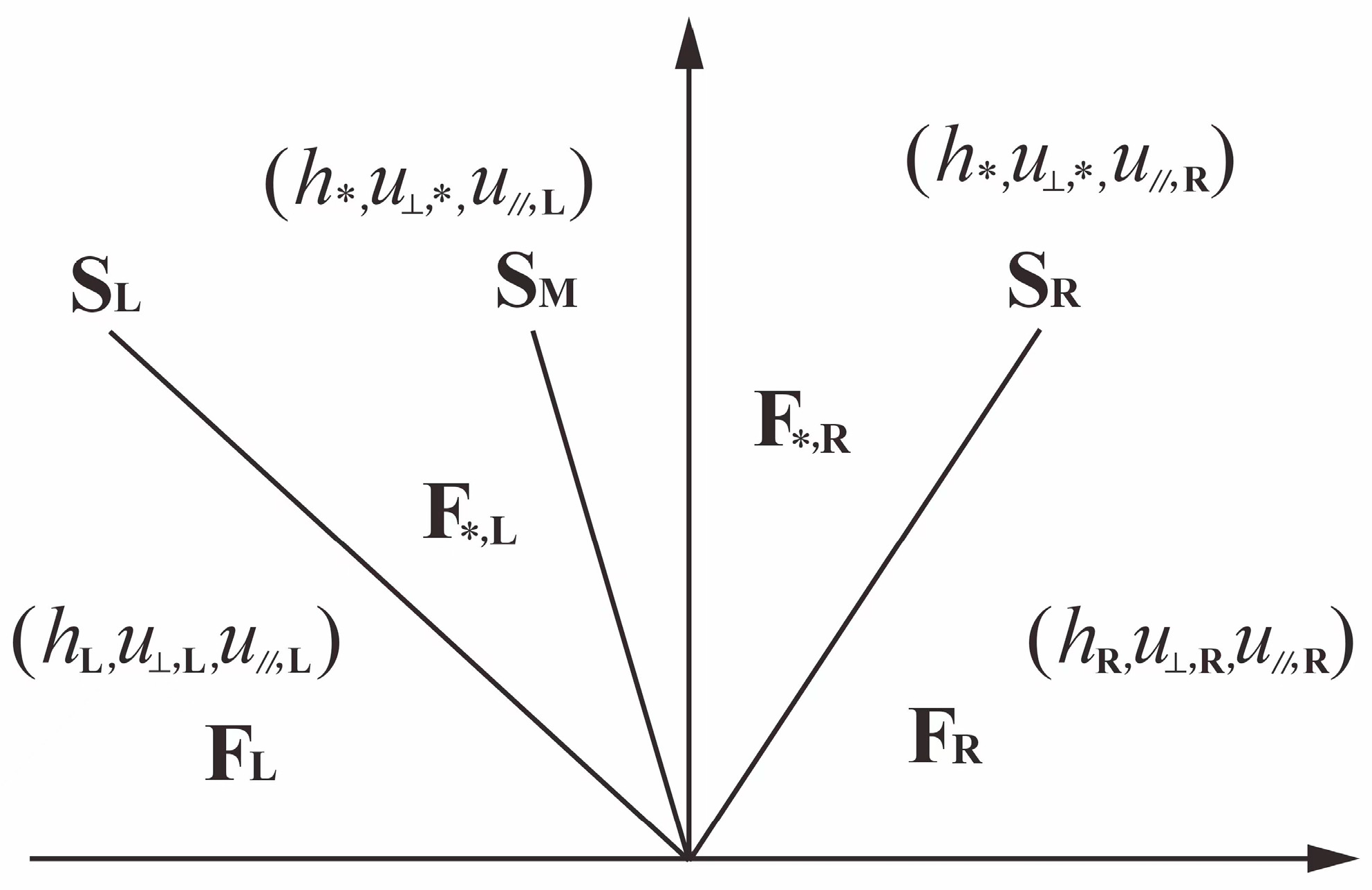
The Harten–Lax–van Leer-Contact (HLLC) scheme is adopted to resolve these Riemann problems due to its computational efficiency and sufficient accuracy for simulation purposes [3,10]. The HLLC scheme satisfies the entropy condition and adapts to wet–dry interface computations when wave speeds are appropriately estimated. The structure of the Riemann solution and the corresponding computational formulas are shown in Figure 2 and expressed as follows:

$$F=\left\{\begin{array}{cc}{F}_L& if 0\le S_L\\ F_{\ast ,L}& if S_L<0\le S_M\\ F_{\ast ,R }& if S_M<0\le S_R\\ F_R & if S_R<0\end{array}\right.$$

(23)

where $S_L$, $S_M$, and $S_R$ are the wave speeds of the left wave, contact wave, and right wave, respectively; $F_L$ and $F_R$ are the numerical fluxes on the left side of the left wave and the right side of the right wave, respectively; and $F_{\ast ,L}$ and $F_{\ast ,R}$ are the numerical fluxes on the left and right sides of the contact wave, respectively. $F_L$ and $F_R$ are calculated as follows:

$$F=\left[\begin{array}{c}h{U}_{\perp }\\ hu{U}_{\perp }+0.5g\left(h^2-b^2\right)n_x\\ hv{U}_{\perp }+0.5g\left(h^2-b^2\right)n_y\end{array}\right]$$

(24)

The numerical fluxes on the left and right sides of the contact wave, denoted as $F_{\ast ,L}$ and $F_{\ast ,R }$, are calculated using Equation (25) and Equation (26), respectively.

$$F_{\ast ,L}=\left[\begin{array}{c}{F}_{\ast ,1}\\ F_{\ast ,2}{n}_x-u_{\parallel ,L}{F_{\ast ,1}n}_y\\ F_{\ast ,2}{n}_y+u_{\parallel ,L}{F_{\ast ,1}n}_x\end{array}\right]$$

(25)

$$F_{\ast ,R}=\left[\begin{array}{c}{F}_{\ast ,1}\\ F_{\ast ,2}{n}_x-u_{\parallel ,R}{F_{\ast ,1}n}_y\\ F_{\ast ,2}{n}_y+u_{\parallel ,R}{F_{\ast ,1}n}_x\end{array}\right]$$

(26)

where $F_{\ast ,1}$ and $F_{\ast ,2}$ are the first and second components of the normal numerical flux calculated using the HLL scheme, respectively.

$$F_{\ast }={\displaystyle \frac{S_R{F}_{\perp ,L}-S_L{F}_{\perp ,R}+S_R{S}_L\left(q_{\perp ,R}-q_{\perp ,L}\right)}{S_R-S_L}}$$

(27)

where $F_{\perp }$ and $q_{\perp }$ can be evaluated with Equations (28) and (29) as

$$F_{\perp }=\left[\begin{array}{c}h\left(u{n}_x+v{n}_y\right)\\ h{\left(u{n}_x+v{n}_y\right)}^2+{\displaystyle \frac{1}{2}}g\left(h^2-b^2\right)\end{array}\right]$$

(28)

$$q_{\perp }=\left[\begin{array}{c}h\\ h\left(u{n}_x+v{n}_y\right)\end{array}\right]$$

(29)

This study adopts the double rarefaction wave assumption and incorporates dry bed conditions to compute left and right wave speeds. The intermediate state is approximated via Roe averaging under the double rarefaction wave assumption, following Einfeldt’s wave speed estimation formula [12].

$$S_L=\left\{\begin{array}{cc}{u}_{\perp ,R}-2\sqrt{g{h}_R}& if h_L=0\\ \mathit{min}\left(u_{\perp ,L}-\sqrt{g{h}_L},u_{\perp ,\ast }-\sqrt{g{h}_{\ast }}\right)& if h_L>0\end{array}\right.$$

(30)

$$S_R=\left\{\begin{array}{cc}{u}_{\perp ,L}+2\sqrt{g{h}_L}& if h_R=0\\ \mathit{max}\left(u_{\perp ,R}+\sqrt{g{h}_R},u_{\perp ,\ast }+\sqrt{g{h}_{\ast }}\right)& if h_R>0\end{array}\right.$$

(31)

$$S_M={\displaystyle \frac{S_L{h}_R\left(u_{\perp ,R}-S_R\right)-S_R{h}_L\left(u_{\perp ,L}-S_L\right)}{h_R\left(u_{\perp ,R}-S_R\right)-h_L\left(u_{\perp ,L}-S_L\right)}}$$

(32)

where the Roe-averaged values of $u_{\perp ,\ast }$ and $h_{\ast }$ can be given as follows:

$$u_{\perp ,\ast }={\displaystyle \frac{\sqrt{h_L{u}_{\perp ,L}}+\sqrt{h_R{u}_{\perp ,R}}}{\sqrt{h_L}+\sqrt{h_R}}}, h_{\ast }={\displaystyle \frac{1}{2}}\left(h_L+h_R\right)$$

(33)

2.6. Source Term Treatment

2.6.1. Slope Source Term Treatment

Since the improved form of the two-dimensional shallow water equations is adopted in this work, the harmonized model does not require any correction terms. A cell-centered approximation method is employed to handle the bed slope term [12]:

$$S_{i,bx}=-{\int }_{\Omega }g\left(h+b\right){\displaystyle \frac{\mathsf{\partial }b}{\mathsf{\partial }x}}d\Omega =-g\left(h+b\right)A_i{\left.{\displaystyle \frac{\mathsf{\partial }b}{\mathsf{\partial }x}}\right|}_i$$

(34)

$$S_{i,by}=-{\int }_{\Omega }g\left(h+b\right){\displaystyle \frac{\mathsf{\partial }b}{\mathsf{\partial }y}}d\Omega =-g\left(h+b\right)A_i{\left.{\displaystyle \frac{\mathsf{\partial }b}{\mathsf{\partial }y}}\right|}_i$$

(35)

2.6.2. Friction Source Term Treatment

Balancing stability and computational efficiency, this study employs the semi-implicit scheme proposed by Wylie and Streeter for handling friction source terms [12].

$$S_{i,fx}=-{\int }_{\Omega }gh{n}^{2}u\sqrt{u^2+v^2}/h^{4/3}d\Omega =-g{n}^2\sqrt{u^2+v^2}/h^{4/3}{\left(hu\right)}^{n+1}$$

(36)

$$S_{i,fy}=-{\int }_{\Omega }gh{n}^{2}v\sqrt{u^2+v^2}/h^{4/3}d\Omega =-g{n}^2\sqrt{u^2+v^2}/h^{4/3}{\left(hv\right)}^{n+1}$$

(37)

2.7. Boundary Conditions

This study employs the direct numerical flux computation method to handle boundary conditions [10,11,25]. Assuming the physical variables on the left side of the boundary are computed using the BIVWLSQ method, the physical variables on the right side are constructed through boundary conditions.

2.7.1. Solid Wall Boundary Condition

For the no-slip boundary condition, both normal and tangential velocities are set to zero, while the water surface elevation and bed elevation on both sides of the boundary are equal. Thus, the physical states on the right side of the boundary are constructed as follows:

$$h_R=h_L,u_{\perp ,R}={-u}_{\perp ,L},u_{\parallel ,R}={-u}_{\parallel ,L}$$

(38)

2.7.2. Free Outflow Boundary Condition

For the free outflow boundary condition, disturbances at this boundary do not affect the flow regime within the computational domain. Therefore, the physical quantities on the right side of the boundary are directly assigned the values from the left side. The formulations are defined as follows:

$$h_R=h_L, u_{\perp ,R}=u_{\perp ,L}, u_{\parallel ,R}=u_{\parallel ,L}$$

(39)

2.7.3. Water Level Boundary Condition

For the water level boundary condition, the temporal variation in the water level is typically prescribed at the boundary. Since the physical variables on the left side of the boundary are known, the right-side variables can be determined using the method of characteristics:

$$h_R=H\left(t\right), u_{\perp ,R}=u_{\perp , L}+2\sqrt{g{h}_L}-2\sqrt{g\left(H\left(t\right)-b_L\right)}, u_{\parallel ,R}=u_{\parallel ,L}$$

(40)

2.7.4. Flow Velocity Boundary Condition

For the flow velocity boundary condition, the normal velocity component $u_{\perp ,R}$ is typically specified on the right side of the boundary. Since the physical quantities on the left side of the boundary are known, they can be determined via the method of characteristics:

$$h_R={\displaystyle \frac{1}{4g}}{\left(u_{\perp ,L}+2\sqrt{g{h}_L}-u_{\perp ,R}\right)}^2$$

(41)

2.7.5. Unit-Width Discharge Boundary Condition

For the unit-width discharge boundary condition, the outward normal unit-width discharge $q_{\perp ,R}=q\left(t\right)$ is typically prescribed at the boundary based on the method of characteristics:

$$2c_R^3-c_R^2\left(u_{\perp ,L}+{2c}_L\right)+g{q}_{\perp ,R}=0$$

(42)

where $c_L$ and $c_R$ are defined as $\sqrt{g{h}_L}$ and $\sqrt{g{h}_R}$, respectively. The value of $c_R$ is solved iteratively using the Newton–Raphson method, and the normal flow velocity is subsequently determined from the known unit-width discharge.

2.7.6. Flow Boundary Condition

This study employs a uniform flow approach for inflow, determines the water levels at the boundaries, distributes hydraulic parameters across the boundary grids, and couples them into the flux computation component of the model [25]. The flow rate for each grid is expressed as:

$$Q_{\perp ,i}=A_{i}C\sqrt{R_{i}J}={\displaystyle \frac{1}{n}}{l}_i{h}_i^{5/3}{J}^{1/2}={\displaystyle \frac{1}{n}}{l}_i{\left(z-z_b\right)}^{5/3}{J}^{1/2}$$

(43)

where $A_i$ is the flow area, $C$ is the Chezy coefficient, and $J$ is the average slope. The total cross-sectional flow rate is given by

$$Q_{\perp }={\displaystyle \frac{1}{n}}{J}^{1/2}{\displaystyle \sum _{i=1}^m}{l}_i{\left(z-z_b\right)}^{5/3}$$

(44)

The binary search method is employed to iteratively approximate the solution of Equation (44), enabling the determination of water levels along the inflow boundary and subsequent derivation of water depths at this boundary. Flow distribution is implemented through Chezy’s formula and Manning’s formula. The formulation is defined as follows:

$$Q_{\perp ,i}={\displaystyle \frac{Q_{\perp }{l}_i{h}_i^{5/3}}{{\sum }_{k=1}^m{l}_k{h}_k^{5/3}}}$$

(45)

Given the known water level and discharge, unit-width discharge and flow velocity are calculated using Equation (46).

$$q_{\perp ,i}={\displaystyle \frac{Q_{\perp }{h}_i^{5/3}}{{\sum }_{k=1}^m\left({l_{k}h}_k^{5/3}\right)}},u_{\perp ,i}={\displaystyle \frac{q_{\perp ,i}}{h_i}}$$

(46)

2.8. Stability Criterion

As an explicit scheme is adopted to solve the shallow water equations, the time step is constrained by stability criteria to ensure numerical stability. The formulation is defined as follows:

$$N_{cfl}=∆t{\displaystyle \frac{\mathit{max}\left(\sqrt{gh}+\sqrt{u^2+v^2}\right)}{\mathit{min}\left(d_{c,LR}\right)}}$$

(47)

where $d_{c,LR}$ is the distance from the cell center to the cell boundary center. When the $N_{cfl}$ number is too large, the propagation speed of physical information will exceed the capture capability of the numerical method, resulting in severe non-physical oscillations in the computational results. When the $N_{cfl}$ number is much smaller than 1, it implies the use of extremely small time steps, which will significantly increase computational time and resource consumption. According to reference [10,13], $N_{cfl}$ is the Courant number specified in the range $0<N_{cfl}\le 1$, and $N_{cfl}=0.5$ is adopted in this work.

3. Test Cases

This section employs a series of benchmark validations comprising analytical solutions, experimental datasets, and field-scale dam-break scenarios with recorded measurements to verify the proposed model. For steady-state simulations, the numerical convergence is evaluated through the global relative error metric. This error metric, formulated by Zhou et al. [29], incorporates volume-weighting for unstructured grids. The formulation is defined as follows:

$$R\left(q\right)=\sqrt{{\displaystyle \frac{{\sum }_i^{N_C}\left[A_i{\left(\frac{q^n-q^{n-1}}{q^n}\right)}^2\right]}{{\sum }_i^{N_c}{A}_i}}}$$

(48)

where $A_i$ is mesh cell area and $N_C$ is number of mesh cells. The numerical solution is deemed to have converged to a steady state when $R\left(h\right)<{10}^{-6}$ is satisfied.

3.1. Preservation of Still Water over a Two-Dimensional Bump

This test case represents a two-dimensional hydrostatic problem with a dry–wet interface over non-flat terrain, aiming to verify that the model exhibits favorable C-property [10,12,30]. The bottom elevation in the test case is

$$\begin{array}{cc}b\left(x,y\right)=\mathit{max}[\mathrm{0,0.25}-5\left({\left(x-0.5\right)}^2+{\left(y-0.5\right)}^2\right)]& 0\le x,y\le 1\end{array}$$

(49)

The computational result is depicted in Figure 3, demonstrating static water levels and a flow rate of 0 m²/s throughout the simulation. These findings confirm that the proposed model achieves robust C-properties in scenarios involving non-flat riverbeds and dry–wet interfaces.

3.2. Oblique Water Leap for Supercritical Flow

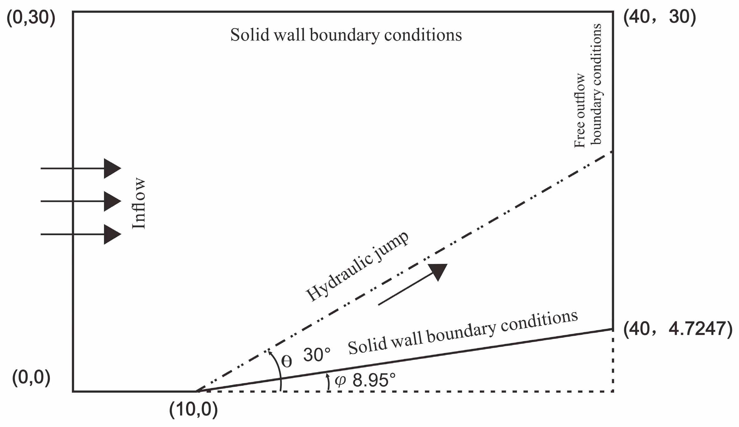
The two-dimensional shallow water equations model developed in this study is validated using a classic oblique hydraulic jump test case. This validation aims to assess the model’s convergence performance and capability in simulating discontinuities within high-velocity flows [13]. The computational domain is illustrated in Figure 4. The initial conditions are specified as follows: water depth = 1 m, inflow velocity = 8.57 m/s, and outflow boundary condition is set as free discharge. Previous studies [30] demonstrate that the angle between the oblique front of the jump and the inflow direction approximates 30°, with the water depth on the upper surface of the jump measuring approximately 1.5 m while the lower surface remains at 1 m. The water depths before and after the jump satisfy the following equation:

$${\displaystyle \frac{h_2}{h_1}}={\displaystyle \frac{1}{2}}\left(\sqrt{1+8F_r^2 {\mathit{sin}}^2\beta }-1\right)$$

(50)

where $h_1$ is the pre-jump water depth, $h_2$ is the post-jump water depth, and $F_r$ is the pre-jump Froude number.

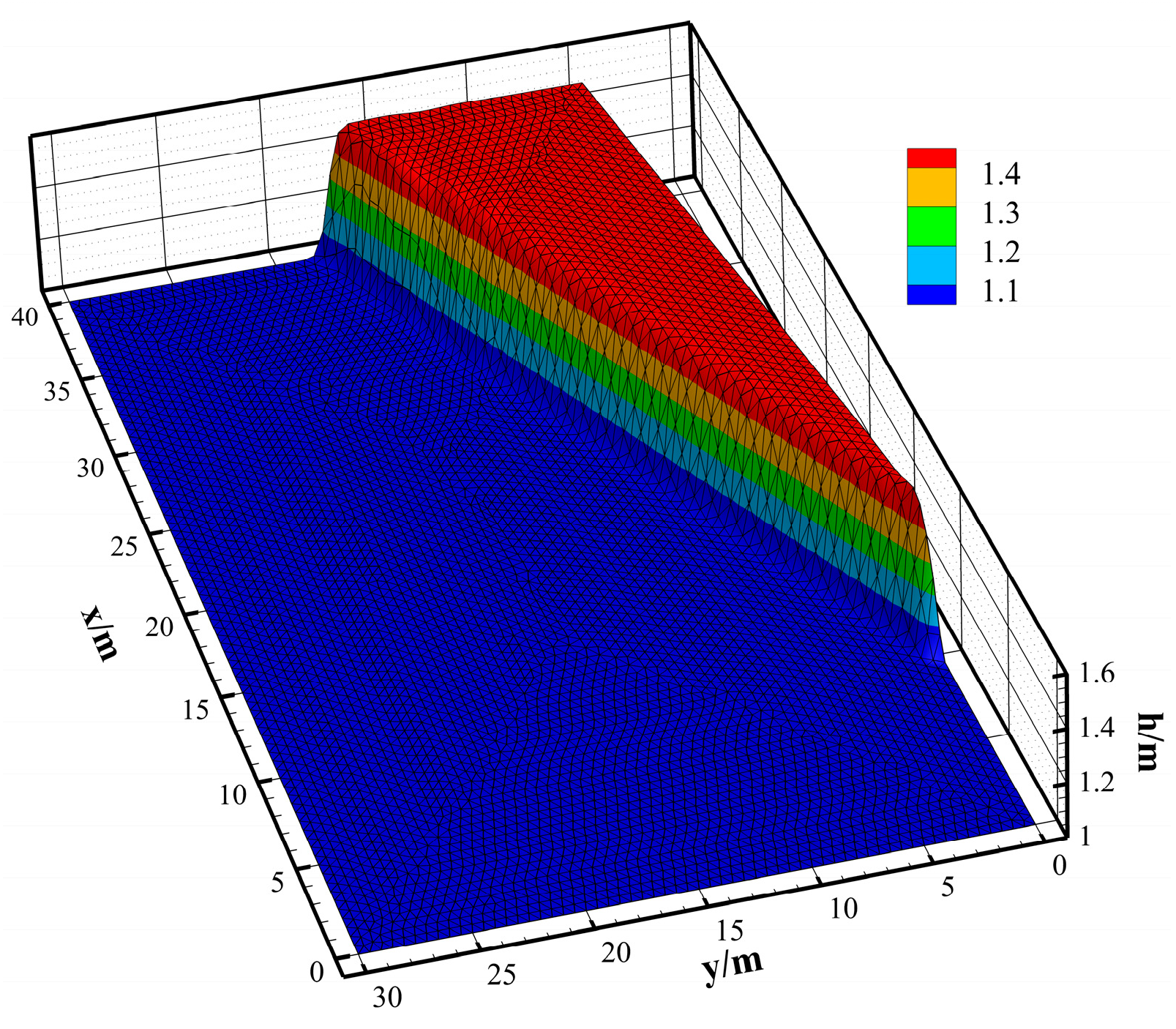
The steady-state results demonstrate an oblique hydraulic jump water depth of $h=1.499$ m (mean absolute error < 0.001) with angle $\theta =30°$, which aligns closely with theoretical and analytical solutions. The corresponding simulation results after stabilization are shown in Figure 5. Compared to Yu et al.’s [13] result of 1.498 m, the model reduces the mean absolute error by 50%.

3.3. Stoker Dam-Break Test Case

The Stoker dam-break test case simulates water flow under flat-bed, resistance-free assumptions. Its theoretical solution, originally derived by Stoker in 1957, is widely adopted for hydrodynamic model validation due to its explicit analytical formulation [13,14]. This study validates the proposed model capability in handling unsteady flow through a rectangular channel measuring 1000 m in length and 100 m in width. A zero-thickness virtual dam is positioned at $x = 500$ m, with initial upstream and downstream water depths set at 5 m and 0.2 m, respectively. Instantaneous dam failure occurs at $t = 0$ s.

Numerical and theoretical solutions for water depth and velocity at t = 20 s, 40 s, and 60 s are compared in Figure 6. The comparative analysis demonstrates strong agreement between model predictions and theoretical benchmarks. Minor numerical oscillations are observed near shock fronts in velocity profiles, though with minimal amplitude. These results confirm the model’s robust accuracy in resolving shock waves and flow discontinuities.

3.4. Two-Dimensional Symmetric Dam-Break Case

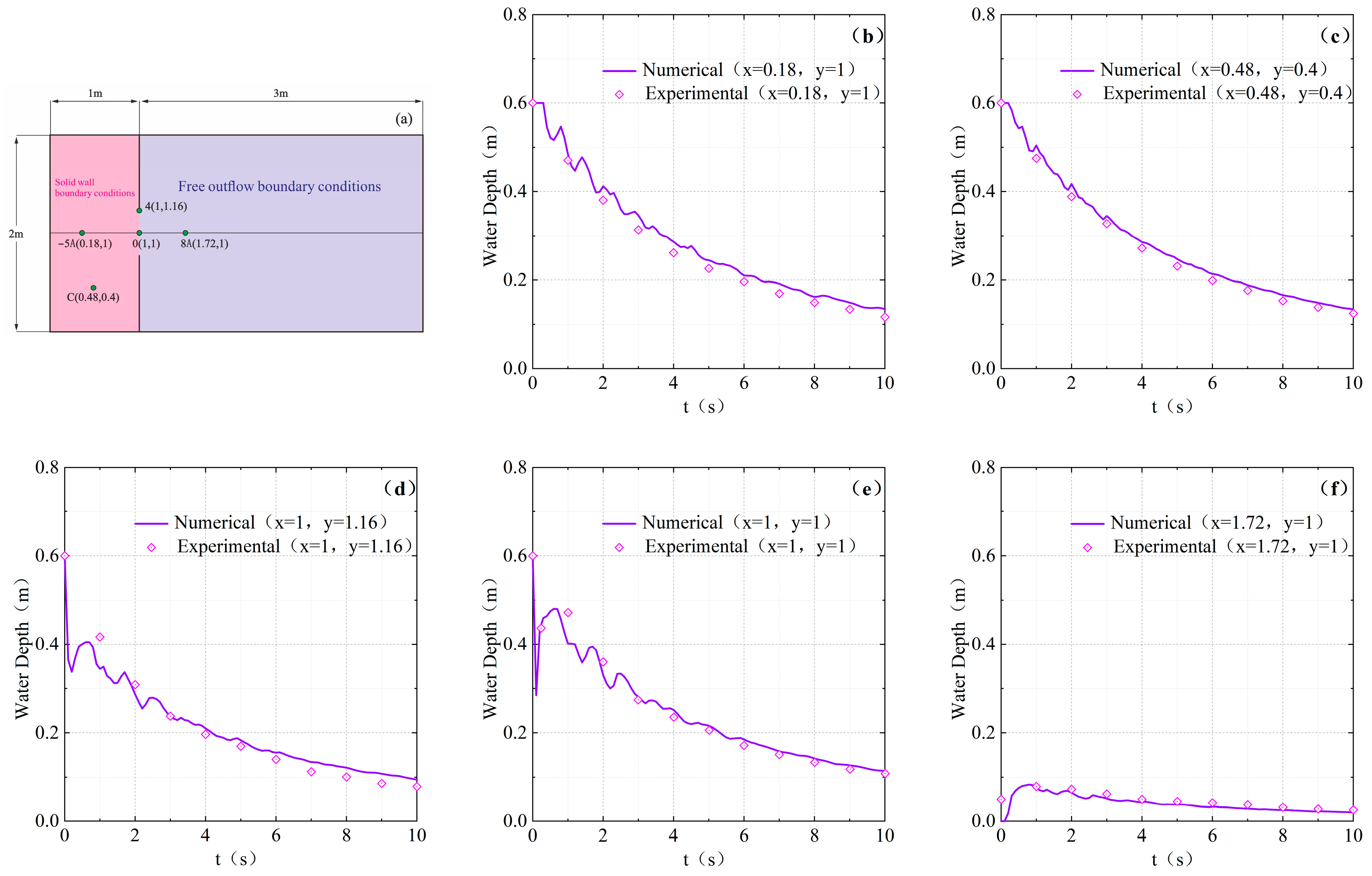
Experimental data from the symmetrical dam-break flume tests conducted by Fraccarollo and Toro [31] are widely used to validate the accuracy of two-dimensional hydrodynamic models [32]. The computational domain is illustrated in Figure 7a. Initial water depths in the upstream and downstream regions are 0.6 m and 0 m, respectively. A 2 m long dam with a symmetrical 0.4 m long central breach connects the reservoir and floodplain, allowing water discharge into the downstream region. The floodplain boundaries employ free outflow conditions on three sides, with the exception of the solid-wall boundary at the dam.

Numerical and experimental water depths at different measurement points are compared in Figure 7. The relative errors at each measurement point are as follows: 7% at point −5A, 6% at point C, 11% at point 4, 6% at point 0, and 18% at point 8A. During the initial phase following dam failure, the flow near the breach exhibits strong three-dimensional characteristics dominated by non-hydrostatic pressure effects. These phenomena cannot be fully captured by the two-dimensional shallow water equations, resulting in slightly underestimated water depths at measurement points 4 and 0 within the first 2 s. Overall, the model demonstrates good agreement with measured water depths across other locations.

3.5. Dam-Break Flow in an L-Shaped Channel

This test case involves a two-dimensional dam-break experiment in an L-shaped 90° curved channel [33,34]. The experimental area comprises a 1.40 m × 1.40 m square reservoir and a 7.25 m long L-shaped 90° curved channel containing six measurement points. The system features flat topography with a Manning coefficient of $n=0.0095 s/m^{1/3}$.

Numerical and experimental solutions are shown in Figure 8. The relative errors at each measurement point are as follows: 0.9% at point P1, 10% at point P2, 8% at point P3, 9% at point P4, 21% at point P5, and 7% at point P6. As demonstrated in Figure 8a–c, measurement points P2, P3, and P4 exhibit two distinct rapid water level rises. The first surge results directly from the abrupt water release following dam failure, while the second arises from flow-blocking effects at the channel’s right-angle bend. Measurement points P5 and P6, located beyond the influence of the bend-induced hydraulic resistance, display only a single rapid water level increase. The model accurately predicts the arrival timings of both flood surges, with numerical solutions at all measurement points showing strong consistency with experimental measurements.

3.6. Toce Urban Inundation Case

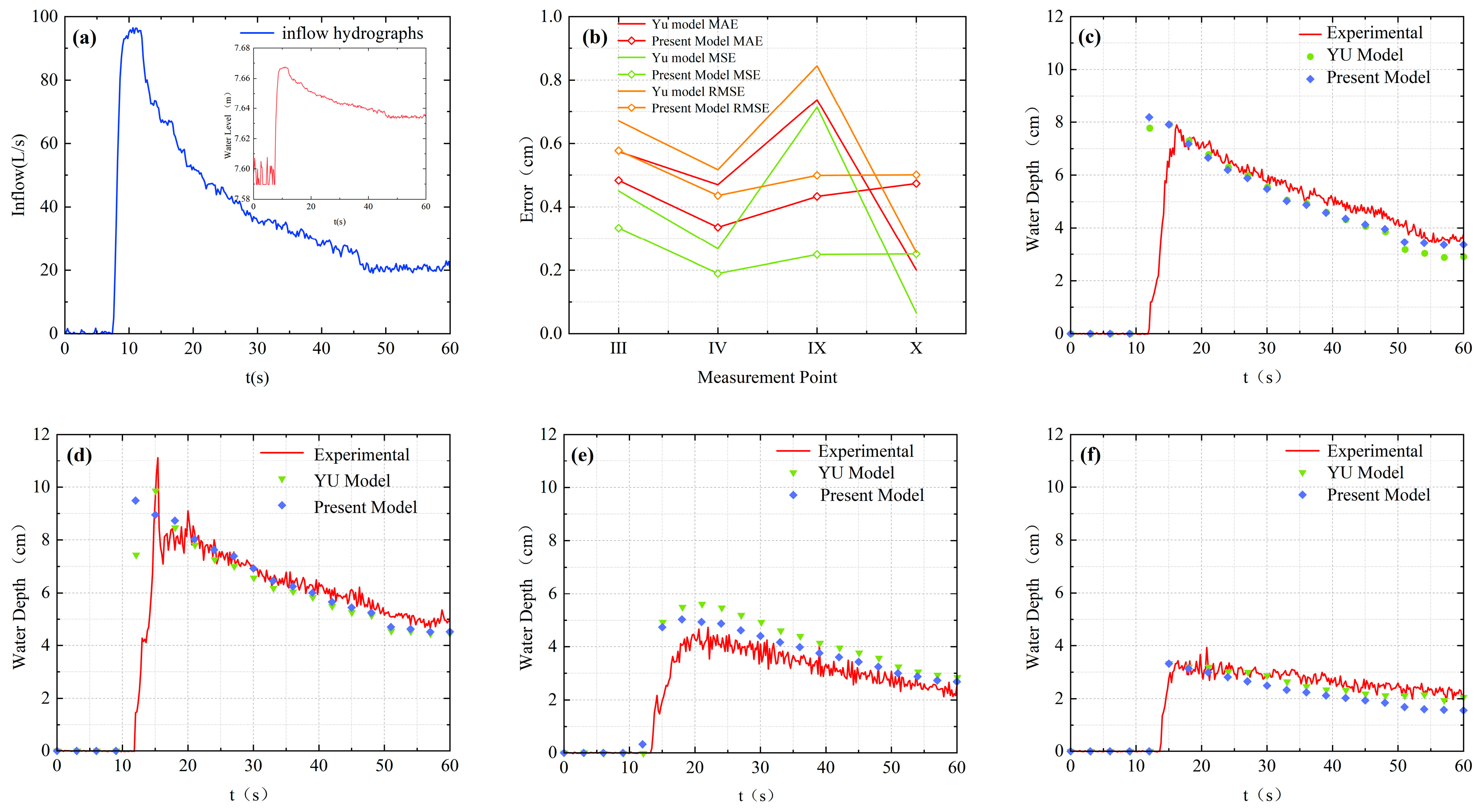
To investigate urban flood propagation characteristics, the Italian CESI (Centro Elettrotecnico Sperimentale Italiano) conducted a series of urban flood simulation experiments [35], which have been widely adopted to validate model applicability in urban areas [36,37,38]. This study selects a regular urban building layout and low inflow conditions for numerical flood simulation to evaluate the capability of the proposed two-dimensional hydrodynamic model in resolving flood dynamics within densely built urban environments. Buildings are treated using the solid-wall boundary method [36]. The upstream inflow and water level conditions derived from the proposed discharge boundary treatment are illustrated in Figure 9a, which exhibit consistent trends.

The entire experimental domain is initially dry. Numerical simulations are performed for 60 s using the proposed model, with results compared against experimental measurements [35] and Yu et al.’s [13] unstructured triangular grid-based solutions. Validation focuses on four measurement points: two upstream of buildings (P3 and P4), one between buildings (P9), and one downstream of buildings (P10), as shown in Figure 9. Error analysis employs three metrics: mean absolute error (MAE), mean squared error (MSE), and root mean squared error (RMSE).

Comparison results at the four measurement points demonstrate strong agreement between the proposed model, experimental data, and literature values. However, due to the model’s second-order accuracy limitations and the inherent constraints of shallow water equations in resolving short-wave dynamics, neither the proposed model nor existing models [13,36,37,38] fully capture rapid water level fluctuations during abrupt discharge reduction and surge phases, a common limitation shared by other two-dimensional shallow water equation-based models [37].

Excluding measurement point P10, the proposed model significantly outperforms the Yu model [13], with overall reductions of 0.2573 cm in MAE, 0.4741 cm in MSE, and 0.2763 in RMSE. Compared to the Yu model, relative improvements reach 12.98% in MAE, 31.67% in MSE, and 12.08% in RMSE. Notably, the absolute error decreases substantially during rapid discharge reduction phases after 40 s.

4. Conclusions

This study resolved the low-accuracy challenge of the second-order cell-centered finite volume method in solving two-dimensional shallow water equations near boundaries. An iterative near-boundary reconstruction method with a nonlinear weighting strategy was developed, coupled with MUSCL-TVD reconstruction in interior regions. A uniform flow-based flux boundary treatment was proposed to ensure conservative allocation of hydraulic parameters, eliminating the need for iterative unit-width discharge calculations. Numerical results demonstrated that the combined BIVWLSQ and MUSCL-TVD reconstruction achieved linear-exact gradients in both interior and near-boundary regions. By integrating a nonlinear weighting strategy inspired by WENO scheme, the method exhibited enhanced shock-capturing capabilities. A uniform flow approach was adopted for dry-bed channels to achieve conservative allocation of hydraulic parameters. This method enhanced flow stability in the inflow region and eliminated the need for iterative unit-width discharge calculations. The computational efficiency was demonstrated to be superior to traditional unit-width discharge calculation methods. The proposed model possessed robust positivity-preserving properties, effectively handled dry-wet interfaces, and maintained strict mass conservation during steady-state convergence. It enabled accurate, stable, and efficient simulations of complex flows over irregular topography in intricate basins. This study still employs classical approaches in temporal discretization schemes and flux calculation methods, and has not yet achieved coordinated optimization across dimensions such as temporal discretization and flux computation. Future work will focus on exploring advanced numerical schemes compatible with these aspects and integrating GPU acceleration technologies to comprehensively enhance the model’s computational performance.

References

1. Zhao, J.; Liang, Q. Novel Variable Reconstruction and Friction Term Discretisation Schemes for Hydrodynamic Modelling of Overland Flow and Surface Water Flooding. Adv. Water Resour. 2022, 163, 104187. [Google Scholar] [CrossRef]
2. Wang, W.; Chen, W.; Huang, G.; Liu, J.; Zhang, D.; Wang, F. A Hybrid Shallow Water Approach with Unstructured Triangular Grids for Urban Flood Modeling. Environ. Model. Softw. 2023, 166, 105748. [Google Scholar] [CrossRef]
3. Aleksyuk, A.I.; Malakhov, M.A.; Belikov, V.V. The Exact Riemann Solver for the Shallow Water Equations with a Discontinuous Bottom. J. Comput. Phys. 2022, 450, 110801. [Google Scholar] [CrossRef]
4. Jian, J.; He, S.; Liu, W.; Liu, S.; Guo, L. A Refined Method for the Simulation of Catchment Rainfall–Runoff Based on Satellite–Precipitation Downscaling. J. Hydrol. 2025, 653, 132795. [Google Scholar] [CrossRef]
5. Diskin, B.; Thomas, J.L.; Nielsen, E.J.; Nishikawa, H.; White, J.A. Comparison of Node-Centered and Cell-Centered Unstructured Finite-Volume Discretizations: Viscous Fluxes. AIAA J. 2010, 48, 1326–1338. [Google Scholar] [CrossRef]
6. Nishikawa, H. From Hyperbolic Diffusion Scheme to Gradient Method: Implicit Green–Gauss Gradients for Unstructured Grids. J. Comput. Phys. 2018, 372, 126–160. [Google Scholar] [CrossRef]
7. Deka, M.; Brahmachary, S.; Thirumalaisamy, R.; Dalal, A.; Natarajan, G. A New Green–Gauss Reconstruction on Unstructured Meshes. Part I: Gradient Reconstruction. J. Comput. Phys. 2020, 422, 108325. [Google Scholar] [CrossRef]
8. Kong, L.; Dong, Y.; Liu, W.; Zhang, H. An Improved Global-Direction Stencil Based on the Face-Area-Weighted Centroid for the Gradient Reconstruction of Unstructured Finite Volume Methods. Chin. Phys. B 2020, 29, 100203. [Google Scholar] [CrossRef]
9. Chen, Z.; Zhang, F.; Liu, J.; Chen, B. A Vertex-Based Reconstruction for Cell-Centered Finite-Volume Discretization on Unstructured Grids. J. Comput. Phys. 2022, 451, 110827. [Google Scholar] [CrossRef]
10. Hou, J.; Liang, Q.; Zhang, H.; Hinkelmann, R. An Efficient Unstructured MUSCL Scheme for Solving the 2D Shallow Water Equations. Environ. Model. Softw. 2015, 66, 131–152. [Google Scholar] [CrossRef]
11. Wang, X.; Hou, J.; Gao, X.; Wang, T.; Zhou, Q.; Li, Y.; Sun, X. Urban Inundation Response Law Analysis to Characteristics of Designed Rainstorms Based on Coupled Hydrodynamic and Rainfall-Tracking Model. J. Hydrol. 2024, 632, 130870. [Google Scholar] [CrossRef]
12. Song, L.; Zhou, J.; Guo, J.; Zou, Q.; Liu, Y. A Robust Well-Balanced Finite Volume Model for Shallow Water Flows with Wetting and Drying over Irregular Terrain. Adv. Water Resour. 2011, 34, 915–932. [Google Scholar] [CrossRef]
13. Yu, H.; Huang, G.; Wu, C. Efficient Finite-Volume Model for Shallow-Water Flows Using an Implicit Dual Time-Stepping Method. J. Hydraul. Eng. 2015, 141, 4015004. [Google Scholar] [CrossRef]
14. Ghoudi, T.; Mohamed, M.S.; Seaid, M. Novel Adaptive Finite Volume Method on Unstructured Meshes for Time-Domain Wave Scattering and Diffraction. Comput. Math. Appl. 2023, 141, 54–66. [Google Scholar] [CrossRef]
15. Wei, Y.; Zhang, F.; Liu, J.; Su, H.; Xu, C. A Constrained Boundary Gradient Reconstruction Method for Unstructured Finite Volume Discretization of the Euler Equations. Comput. Fluids 2023, 252, 105774. [Google Scholar] [CrossRef]
16. May, S.; Berger, M. Two-Dimensional Slope Limiters for Finite Volume Schemes on Non-Coordinate-Aligned Meshes. SIAM J. Sci. Comput. 2013, 35, A2163–A2187. [Google Scholar] [CrossRef]
17. Wang, Q.; Ren, Y.; Pan, J.; Li, W. Compact High Order Finite Volume Method on Unstructured Grids III: Variational Reconstruction. J. Comput. Phys. 2017, 337, 1–26. [Google Scholar] [CrossRef]
18. Zhang, F.; Liu, J.; Chen, B. Modified Multi-Dimensional Limiting Process with Enhanced Shock Stability on Unstructured Grids. Comput. Fluids 2018, 161, 171–188. [Google Scholar] [CrossRef]
19. Li, Z.; Ou, G.; Chen, L.; Ji, W.; Tao, W. An Implicit Scheme for Least-Square Gradient in Coupled Algorithm. Int. J. Numer. Methods Fluids 2025, 97, 795–819. [Google Scholar] [CrossRef]
20. Li, T.; Zou, Y.; Zou, S.; Chang, X.; Zhang, L.; Deng, X. Learning to Solve PDEs with Finite Volume-Informed Neural Networks in a Data-Free Approach. J. Comput. Phys. 2025, 530, 113919. [Google Scholar] [CrossRef]
21. Chen, Z.; Zhang, F.; Liu, J.; Chen, B. An Iterative Near-Boundary Reconstruction Strategy for Unstructured Finite Volume Method. J. Comput. Phys. 2020, 418, 109621. [Google Scholar] [CrossRef]
22. Nishikawa, H.; White, J.A. An Efficient Cell-Centered Finite-Volume Method with Face-Averaged Nodal-Gradients for Triangular Grids. J. Comput. Phys. 2020, 411, 109423. [Google Scholar] [CrossRef]
23. Zhang, J.; Xia, Y.; Xu, Y. Structure-Preserving Finite Volume Arbitrary Lagrangian-Eulerian WENO Schemes for the Shallow Water Equations. J. Comput. Phys. 2023, 473, 111758. [Google Scholar] [CrossRef]
24. Liu, X.; Osher, S.; Chan, T. Weighted Essentially Non-oscillatory Schemes. J. Comput. Phys. 1994, 115, 200–212. [Google Scholar] [CrossRef]
25. Hou, J.; Wang, Y.; Zhang, Z.; Li, B.; Wang, J.; Zhang, D. Inflow Boundary Optimized Method in Two-dimensional Hydrophobic Model. Adv. Eng. Sci. 2022, 54, 39–46. [Google Scholar] [CrossRef]
26. Ru, Z.; Liu, H.; Tu, G.; Huang, W. Water-Balanced Inlet and Outlet Boundary Conditions of the Lattice Boltzmann Method for Shallow Water Equations. Comput. Fluids 2023, 256, 105860. [Google Scholar] [CrossRef]
27. Zia, A.; Banihashemi, M.A. Simple Efficient Algorithm (SEA) for Shallow Flows with Shock Wave on Dry and Irregular Beds. Int. J. Numer. Methods Fluids 2008, 56, 2021–2043. [Google Scholar] [CrossRef]
28. Ghaeini-Hessaroeyeh, M.; Namin, M.M.; Fadaei-Kermani, E. 2-D Dam-Break Flow Modeling Based on Weighted Average Flux Method. Iran. J. Sci. Technol. Trans. Civ. Eng. 2021, 46, 1515–1525. [Google Scholar] [CrossRef]
29. Zhou, J.G.; Causon, D.M.; Mingham, C.G.; Ingram, D.M. The Surface Gradient Method for the Treatment of Source Terms in the Shallow-Water Equations. J. Comput. Phys. 2001, 168, 1–25. [Google Scholar] [CrossRef]
30. Wang, X.; Chen, G. Well-Balanced and Positivity-Preserving Wet-Dry Front Reconstruction Scheme for Ripa Models. Appl. Numer. Math. 2025, 213, 38–60. [Google Scholar] [CrossRef]
31. Fraccarollo, L.; Toro, E.F. Experimental and Numerical Assessment of the Shallow Water Model for Two-Dimensional Dam-Break Type Problems. J. Hydraul. Res. 1995, 33, 843–864. [Google Scholar] [CrossRef]
32. O’Dea, E.; Bell, M.J.; Coward, A.; Holt, J. Implementation and Assessment of a Flux Limiter Based Wetting and Drying Scheme in NEMO. Ocean Model. 2020, 155, 101708. [Google Scholar] [CrossRef]
33. Gottardi, G.; Venutelli, M. Central Scheme for Two-Dimensional Dam-Break Flow Simulation. Adv. Water Resour. 2004, 27, 259–268. [Google Scholar] [CrossRef]
34. Ion, S.; Marinescu, D.; Cruceanu, S.-G. Numerical Scheme for Solving a Porous Saint-Venant Type Model for Water Flow on Vegetated Hillslopes. Appl. Numer. Math. 2022, 172, 67–98. [Google Scholar] [CrossRef]
35. Testa, G.; Zuccalà, D.; Alcrudo, F.; Mulet, J.; Soares-Frazão, S. Flash Flood Flow Experiment in a Simplified Urban District. J. Hydraul. Res. 2007, 45, 37–44. [Google Scholar] [CrossRef]
36. Kim, B.; Sanders, B.F.; Schubert, J.E.; Famiglietti, J.S. Mesh Type Tradeoffs in 2D Hydrodynamic Modeling of Flooding with a Godunov-Based Flow Solver. Adv. Water Resour. 2014, 68, 42–61. [Google Scholar] [CrossRef]
37. Costabile, P.; Costanzo, C.; De Lorenzo, G.; Macchione, F. Is Local Flood Hazard Assessment in Urban Areas Significantly Influenced by the Physical Complexity of the Hydrodynamic Inundation Model? J. Hydrol. 2020, 580, 124231. [Google Scholar] [CrossRef]
38. Saleem, M.W.; Rashid, M.; Haider, S.; Khalid, M.; Elfeki, A. Simulation of Urban Flooding Using 3D Computational Fluid Dynamics with Turbulence Model. Results Eng. 2025, 25, 103609. [Google Scholar] [CrossRef]
Figure 1. The BIVWLSQ method template used in the model between variable f and position vector r.
Jmse 13 02036 g001
Figure 2. Riemann solution structure between left wave S L , contact wave S M , right wave S R , flux F, Water depth h, and flow velocity u.
Jmse 13 02036 g002
Figure 3. Comparison of analytical and numerical solutions of water level and unit width discharge at convergence in the y = 0.5 m cross-section.
Jmse 13 02036 g003
Figure 4. Experimental configuration for oblique water leap for supercritical flow.
Jmse 13 02036 g004
Figure 5. Water depth contour plot of the oblique hydraulic jump at convergence.
Jmse 13 02036 g005
Figure 6. Comparison of numerical and theoretical solutions (a) 20 s, (b) 40 s, and (c) 60 s.
Jmse 13 02036 g006
Figure 7. Experimental model and comparison of numerical and experimental solutions (a) model computational domain, (b) −5A, (c) C, (d) 4, (e) 0, (f) 8A.
Jmse 13 02036 g007
Figure 8. Comparison of numerical and experimental solutions (a) P1, (b) P2, (c) P3, (d) P4, (e) P5, (f) P6.
Jmse 13 02036 g008
Figure 9. Inflow curve and comparison of numerical and experimental solutions (a) inflow curve, (b) error comparison, (c) P3, (d) P4, (e) P5, (f) P6.
Jmse 13 02036 g009
Disclaimer/Publisher’s Note: The statements, opinions and data contained in all publications are solely those of the individual author(s) and contributor(s) and not of MDPI and/or the editor(s). MDPI and/or the editor(s) disclaim responsibility for any injury to people or property resulting from any ideas, methods, instructions or products referred to in the content.