Abstract
Understanding the variability of turbulence intensity (TI) under different wind regimes is essential for the design and safety of offshore wind turbines. The IEC Normal Turbulence Model (NTM), though widely adopted in industry, does not incorporate directional dependence or account for extreme wind events such as typhoons, which can lead to substantial underestimation of turbulence in complex offshore environments. In this study, field measurements from two coastal sites in China, Huilai and Pingtan, were analyzed. At Pingtan, two months of observations captured both normal and typhoon-affected winds, providing a unique dataset for assessing turbulence under typhoon-affected conditions. The results show that wind speeds during the typhoon-affected period were approximately 14% higher than those during normal periods. At Huilai, TI was evaluated under northeasterly and southeasterly sea breezes, revealing that the IEC NTM underestimated TI by 15–42%, with more pronounced discrepancies under northeasterly winds. Based on these findings, revised NTM parameters and correction factors are proposed for different wind conditions, enhancing the applicability of the model to offshore wind turbine design. This work underscores the importance of incorporating directional and event-specific modifications into IEC turbulence standards to ensure reliable structural assessment across diverse wind regimes.
1. Introduction
Wind turbulence is one of the most critical factors influencing the aerodynamic performance and structural safety of wind turbines. It directly drives unsteady aerodynamic loads, accelerates fatigue damage, and shortens turbine service life. This issue is particularly important for offshore wind turbines, which are increasingly deployed in regions with complex meteorological conditions and highly variable marine boundary layers. With the rapid global expansion of offshore wind energy as a cornerstone of carbon-neutral energy transition, the ability to accurately model turbulence has become essential for both resource assessment and reliable turbine design [1].
While standardized models such as the IEC Normal Turbulence Model (NTM) are widely used in design practices [2,3], they are predominantly derived from onshore measurement data and assume stationary, Gaussian-distributed turbulence with predefined empirical parameters [4,5,6]. These assumptions may not adequately represent the physical characteristics of turbulence in coastal and offshore environments, where mesoscale processes and marine boundary layer dynamics play a critical role [7,8]. The offshore boundary layer is often characterized by different thermal stratification, lower surface roughness, and higher wind shear compared with onshore environments. Processes such as sea-air temperature differences lead to stable or convective conditions that alter turbulence generation and dissipation mechanisms.
Numerous field studies have demonstrated that offshore turbulence often exhibits pronounced non-Gaussian features, such as intermittency [9], high kurtosis [10], and asymmetry [11]. These deviations are particularly evident under stable or transitional stratification, where mixing mechanisms differ from those in terrestrial turbulence. In addition, typhoon-induced turbulence introduces further modeling challenges: field campaigns have shown that turbulence intensity, gust factors, and integral length scales during typhoon events far exceed those under non-cyclonic conditions [12,13]. Lin reported specific wind characteristics during typhoons according to the field measurements in Pingtan, China [14]. Qin emphasized the non-stationary nature of typhoon winds [15].
To reduce these discrepancies, recent research has increasingly focused on recalibrating turbulence models using site-specific observations. Ishihara [16] and Leu [17] analyzed wind data from offshore platforms and compared the observed turbulence intensity with the IEC regulations, while Dai [18,19] further segregated sea breeze and land breeze based on wind direction data, thereby comparing their differences in turbulence intensity. Cheng investigate the wind speed data in coastal areas indicate the effort of land–sea breeze for wind energy development [20]. Large-eddy simulations combined with field data have also been used to explore wake alignment and directional variability [21,22]. These studies consistently indicate that the IEC model underestimates offshore turbulence and turbine loads, particularly under monsoon, sea breeze, and typhoon conditions.
Despite these advances, there is still limited evidence combining both typhoon-affected measurements and seasonal sea breeze variability, which are highly relevant for the rapidly growing offshore wind sector in East Asia. To address these open questions discussed above, the present study conducted field measurement campaigns at two representative offshore sites in the southeastern coastal regions (Figure 1): Huilai, which exhibits strong directional wind effects due to monsoon and topographic influences; and Pingtan, which experiences both typical marine and typhoon wind conditions. Unlike approaches that rely on pre-averaged or lower-frequency data, this study deploys high-precision instruments sampling at 1 Hz that enables the direct computation of turbulence statistics from the raw data. This method effectively avoids the potential smoothing effect and loss of turbulent fluctuations inherent in using mean values (e.g., 2 min or 10 min mean wind speed), leading to a more accurate and fundamental determination of parameters like turbulence intensity.
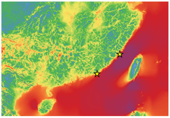
Figure 1.
Distribution of mean wind speed and two filed measurement campaign locations along the southeast coast of China.
Based on the observed differences in wind statistics between these sites, targeted analyses are performed to investigate turbulence properties, wind veer and directional variability, and the influence of extreme wind events. The objective of this study is to recalibrate the IEC Normal Turbulence Model using rare typhoon-affected and seasonal sea breeze datasets and to propose revised parameterizations that better represent offshore turbulence for wind turbine design. Referring to the previous approach [16,17,18,19], this study creates a unified recalibration that accounts for both extreme events and seasonal variability.
The remainder of this paper is structured as follows: Section 2 introduces the fundamentals of turbulence modeling and the field observation setup. Section 3 describes the data processing methodology and presents the parameter calibration results. Section 4 concludes with key findings and future work.
2. Methodology
2.1. Overview of the IEC NTM Model
The International Electrotechnical Commission (IEC) has developed a comprehensive series of standards for wind turbines, such as IEC 61400-1 for design requirements and IEC 61400-12-1 for power performance testing. These standards are widely adopted across the wind energy industry to ensure consistency and reliability in wind turbine assessment and certification [2,3]. According to IEC 61400-12-1, which governs the power performance measurement of electricity-producing wind turbines, wind speed data should be collected continuously at a sampling frequency of at least 1 Hz. The data acquisition system is required to record either the raw high-frequency measurements or aggregated 10 min statistics. Each 10 min data block must include key indicators such as the mean wind speed, standard deviation, and maximum and minimum wind speeds.
For subsequent analysis, the collected data are segmented into non-overlapping 10 min intervals, which represent the standard time base for wind resource assessment and load simulation. The mean wind speed and standard deviation for each interval are computed using the following formulations:
where is the number of original measured data within the 10 min period, is the original measured data sample, is the mean wind speed of the 10 min period, and is the standard deviation of the 10 min period.
TI is a key parameter for characterizing the level of wind turbulence and is defined as the ratio of the standard deviation of wind speed to its corresponding mean value, expressed as:
According to IEC 61400-1, the Normal Turbulence Model (NTM) is recommended for characterizing turbulence under standard wind conditions. Within the NTM framework, the representative turbulence intensity value, denoted as , corresponds to the 90th percentile of the standard deviation of the longitudinal wind component. IEC standards define three primary components of turbulence standard deviation: , , and are defined as the longitudinal (main wind direction), lateral, and upward wind velocity standard deviation, respectively. The mean and standard deviation values of turbulence standard deviation is often assumed to follow a log-normal distribution, which enables the derivation of its mean and standard deviation for different turbulence classes. The distribution parameters can be approximated using the following expressions [2]:
where and are the mean and standard deviation value of wind speed standard deviation , is the reference value of the turbulence intensity, is the mean wind speed, and , , , and are the model parameters. According to the IEC regulations [2,3], the value of reference turbulence intensity is based on three categories: higher (A), medium (B), and low (C) turbulence characteristics. The value of of each category is 0.16, 0.14, and 0.12.
The mean wind speed dataset is analyzed using the ‘Method of Bins’, which segments the wind speed range into contiguous intervals of 1 m/s, each centered at an integer wind speed (e.g., 5.0 m/s, 6.0 m/s, etc.). Within each bin, the probability density function (PDF) of the mean wind speed is computed, allowing for a detailed statistical characterization of wind speed distribution across the observed range. To evaluate the turbulence characteristics, the 90th percentile of the turbulence standard deviation is calculated for each bin. Under the assumption that turbulence fluctuations follow a normal distribution, serves as a representative upper bound metric. This parameter is particularly important for estimating extreme fatigue loads and guiding the structural design of wind turbines. The mathematical formulation for is given by:
where and are the mean and standard deviation of the turbulence standard deviation within each wind speed bin. The factor 1.28 corresponds to the z-score of the 90th percentile for a standard normal distribution.
Substitute Equations (4) and (5) into Equation (6). The 90th percentile of turbulence standard deviation can be formulated as:
Thus, the turbulence intensity can be calculated as:
2.2. Field Observation Campaign
As part of this study, two field observation campaigns were carried out to investigate the higher-order statistical characteristics of natural wind. The first campaign was conducted in Pingtan, Fujian Province, from August to September 2023, covering a 2-month period including Typhoon Haikui. The second campaign was then conducted in Huilai County, Guangdong Province, from June 2024 to May 2025, covering one full year to capture seasonal directional variability. Both campaigns continuously recorded wind speed and direction at a sampling frequency of 1 Hz using anemometer-based instrumentation, including an ultrasonic anemometer and a cup anemometer. The choice of 1 Hz sampling complies with the minimum requirement specified in IEC 61400-12-1 for power performance assessment, particularly when high-frequency turbulence data are unavailable.
The monitoring stations were carefully selected to minimize topographical interference and ensure unobstructed wind exposure. At Pingtan, the weather station was installed on the rooftop approximately 100 m from the shoreline (Figure 2a). At Huilai, the station was mounted on the rooftop about 600 m from the shoreline (Figure 2b). The instrumentation setups for both sites were designed to optimize measurement accuracy and minimize interference. At Pingtan and Huilai, the instruments were installed 25 m and 44 m above ground, which are both on the rooftop of the tallest buildings in the surrounding area (Figure 2c). The T-bar structures oriented toward the prevailing sea breeze direction with no nearby obstructions or tall buildings. The cup and ultrasonic anemometers were mounted with sufficient separation to minimize aerodynamic interference (Figure 2d,e).
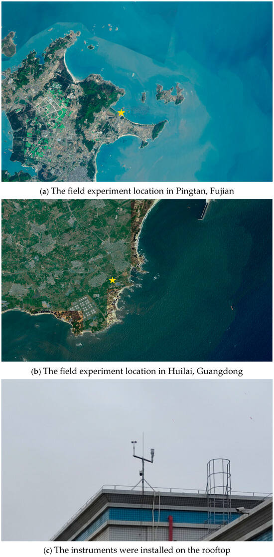
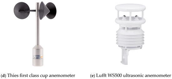
Figure 2.
Field measurement setup and anemometers.
Wind speed data were primarily recorded using a Thies first class cup anemometer (Adolf Thies GmbH & Co. KG, Göttingen, Germany), while a Lufft WS500 ultrasonic anemometer (OTT HydroMet Fellbach GmbH, Kempten, Germany) served as a backup sensor. In addition to wind speed, the ultrasonic anemometer continuously recorded supplementary meteorological parameters, including wind direction, temperature, humidity, and atmospheric pressure. Although meteorological data such as temperature, humidity, and atmospheric pressure is not included in this study, we recognize that collecting this data would have been beneficial for analyzing the impact of seasonal changes on the wind speed model. The key technical specifications of both instruments are summarized in Table 1.

Table 1.
Technical specifications of anemometers.
2.3. Data Processing
2.3.1. Post-Process Method
To ensure compliance with IEC international standards for wind data analysis and turbulence characterization, a comprehensive post-processing methodology is implemented in this study. This method addresses the requirements of IEC 61400-12-1 for power performance assessment and IEC 61400-1 for turbulence model evaluation, providing a standardized and reproducible framework for offshore wind resource assessment [14,15]. The proposed procedure consists of the following steps:
- 1.
- Step 1: Data Segmentation and Pre-Processing
Continuous wind speed time histories recorded at 1 Hz are divided into non-overlapping 10 min segments, corresponding to the standard reference interval adopted in wind engineering. This segmentation results in 600 samples per segment in this study. The use of 10 min blocks is critical because many wind statistics, such as turbulence intensity and gust factors, are defined for 10 min periods in IEC standards. Prior to segmentation, raw data are screened for obvious anomalies (e.g., sensor errors recorded as 99, 999 or N/A) using threshold filters, ensuring consistency and reliability for subsequent analysis.
- 2.
- Step 2: Statistical Computation of Wind Parameters
For each segment, the 10 min mean wind speed, standard deviation, and mean wind direction are computed using Equations (1)–(3).
- 3.
- Step 3: Directional Filtering
To isolate coastal wind regimes of interest, only segments with mean wind directions within predefined sea breeze boundaries are retained. This ensures that subsequent statistical evaluation focuses exclusively on periods dominated by offshore flow, which is critical for nearshore wind energy applications.
- 4.
- Step 4: Stationarity Assessment
A key requirement for turbulence characterization is that wind speed time series are statistically stationary over the averaging interval. To assess this, the Reverse Arrangement Test (RAT) is applied to exclude non-stationary segments, ensuring that the turbulence samples used for regression were representative and reliable for NTM recalibration. Originally introduced by Kendall nd later refined by Mann, the RAT is a nonparametric rank-based test designed to detect monotonic trends in time series data [23].
For a segment of size , the RAT test statistic counts the number of inversions (reverse arrangements) in the sequence. The expected value and variance of under the null hypothesis (stationarity) are:
The standardized test statistic is given by:
At a 95% confidence level, segments satisfying are considered stationary.
- 5.
- Step 5: Method of Bins and Turbulence Characterization
For segments passing the stationarity criterion, the Method of Bins [2] is employed to group standard deviations according to mean wind speed bins (typically 1 m/s intervals). Within each bin, the following parameters , , and are computed.
- 6.
- Step 6: Advanced Analysis for Offshore Wind Design
Beyond basic turbulence characterization, the processed data allow further derivation of turbulence intensity and directional variability, which are critical for site classification, load modeling, and probabilistic reliability assessments.
2.3.2. Software Implementation
The entire post-processing chain is automated using STORM (Statistic, Turbulence, Open-field, Record, Measurement), a custom-built tool developed in this study. STORM includes the following components:
- Data Loading and Quality Control: Handles raw SCADA or logger data and applies plausibility checks;
- Stationarity Testing Module: Implements RAT with graphical diagnostics (z-value distribution plots);
- Statistical Aggregation: Automates the Method of Bins and computes turbulence parameters;
- Regulatory Compliance: Cross-checks processed results against IEC 61400 thresholds;
- Visualization Tools: Provides figures for wind roses, TI curves, z-value histograms, and bin-wise turbulence plots.
Unlike traditional spreadsheet-based processing, STORM significantly reduces manual effort and computational errors, enabling the efficient handling of large datasets while maintaining full traceability and reproducibility.
3. Results
3.1. Extreme Conditions of Field Observation at Pingtan, Fujian
Typhoon Haikui originated as a tropical depression over the western North Pacific on 27 August 2023 and gradually intensified while moving west–northwest. By September 3, it had reached category 3 equivalent strength, with maximum sustained winds up to approximately 195 km/h near its core. The path of Typhoon Haikui (2023), including its trajectory across Taiwan and final landfall in Fujian, is illustrated in Figure 3. The storm center is approximately 200 km south of the measurement site when it passed through. Therefore, the captured data is valuable for evaluating turbulence under typhoon-affected conditions rather than true extreme winds.
Figure 3.
Path of Typhoon Haikui.
To further utilize this valuable dataset, the wind speed observations were systematically classified into two distinct groups: typhoon-affected and normal sea breeze. Specifically, the period from 31 August to 5 September 2023 was designated as the Typhoon Haikui group, while the remaining days were assigned to the normal sea breeze group. In both cases, the prevailing wind direction was around 25°, nearly perpendicular to the coastline. Since Typhoon Haikui passed south of the site, its main impact was to increase wind speed through outer circulation rather than to change wind direction.
In order to compare with the IEC turbulence models, the turbulence intensities for NTM Models A, B, and C of each bin are calculated using Equation (7) and parameters in IEC regulations [2]. The turbulence intensity curves for NTM Models A, B, and C are represented as red, green, and blue dashed lines, respectively. Additionally, the 90th percentile of the measured turbulence intensity curve is represented by a black dashed line and the turbulence intensities of original 10 min segments of Typhoon Haikui are calculated and represented as pink crosses in Figure 4.
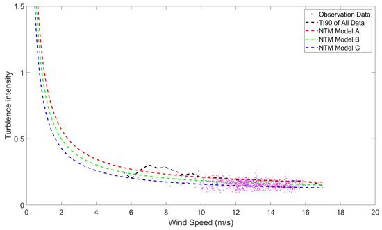
Figure 4.
Turbulence intensities of typhoon-affected sea breeze.
It is evident that the wind speed measurements during the passage of Typhoon Haikui were predominantly concentrated in the range of 10–16 m/s, which is markedly higher than the long-term average wind speed at the site. Data samples below 10 m/s were relatively scarce, and therefore the corresponding turbulence intensity values are of limited reference value. Focusing on wind speeds above 10 m/s, the 90th percentile of the observed turbulence intensity closely matches that predicted by NTM Model A, with the two distributions nearly overlapping. It should be noted that the recorded wind data corresponds to the outer circulation of Typhoon Haikui rather than its eyewall or central core. For the wind data captured from the central region of the typhoon, the new IEC turbulence category A+ is recommended for the recalibration analysis.
The results of the turbulence intensity of typhoon-affected sea breeze and NTM Model A are shown in Table 2.
Table 2.
Turbulence intensity of typhoon-affected sea breeze.
Similar procedures are conducted for normal sea breeze, and the results are presented in Figure 5.
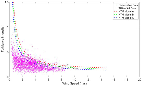
Figure 5.
Turbulence intensities of normal sea breeze.
In contrast, the wind speed measurements outside the typhoon-affected period were primarily concentrated below 8 m/s, which is consistent with the site’s typical wind regime. Analysis of the observational results indicates that the 90th percentile curve of observed TI lies between NTM Models A and B, aligning more closely with Model B for wind speeds above 6 m/s. This suggests that NTM Model B provides a more appropriate representation of the local wind characteristics.
The results of the turbulence intensity of normal sea breeze and NTM Model B are shown in Table 3.
Table 3.
Turbulence intensity of normal wind.
3.2. Directional Variablity of Field Observation at Huilai, Guangdong
According to the monthly wind rose analysis, the prevailing wind at Huilai is northeast throughout the year, especially in winter, while in summer the dominant wind occasionally shifts to southeast for about one month, as shown in Figure 6a. The main direction of the northeast sea breeze in this study is approximately 65°. To ensure that the majority of the sea breeze component is captured, a wind direction range of ±35° from the central direction is defined (Figure 6b). In addition, the main direction of the southeast sea breeze is 150°, with a wind direction range of ±50° (Figure 6c).
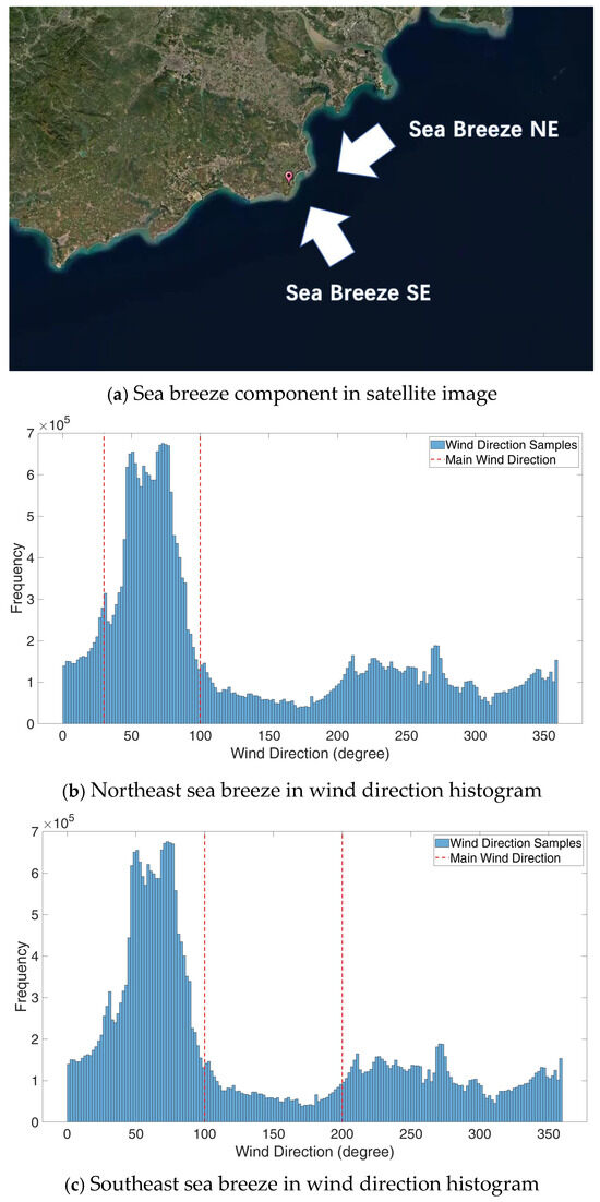
Figure 6.
Sea breeze in wind direction histogram.
The turbulence intensity curves for NTM Models A, B, and C are represented as a red, green, and blue dashed line in Figure 7, respectively. Additionally, the 90th percentile of the measured turbulence intensity curve is represented by a black dashed line and the turbulence intensities of original 10 min segments of sea breeze are calculated and represented as pink crosses. The results of stationary and non-stationary data of northeast sea breeze are presented in Figure 7a,b, respectively.
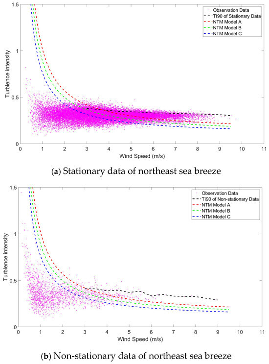
Figure 7.
Turbulence intensities of northeast sea breeze.
It is clear that all three Normal Turbulence Models (NTMs) consistently underestimate turbulence intensity when compared with field measurement data, aligning with findings reported in prior studies [16]. However, the degree of underestimation observed in our coastal site for northeasterly winds (15–42%) is substantially more severe than the 10–20% reported in their open-sea study [16]. This discrepancy is likely due to the channeling effect of the Taiwan Strait and land–sea interactions. Specifically, the 90th percentile of the observed turbulence intensity exceeds that of Model A by approximately 15% at 5 m/s and by 42% at 9 m/s. Moreover, while the turbulence intensity predicted by NTM Model A decreases steadily as wind speed increases, the turbulence intensity derived from field data remains relatively stable across the same range, consistent with recent observations in offshore wind environments [24].
The results of the turbulence intensity of stationary northeast sea breeze are shown in Table 4.
Table 4.
Turbulence intensity of stationary data for northeast sea breeze.
Similar procedures are conducted for southeast sea breeze, and the results are presented in Figure 8. The results of stationary and non-stationary data of southeast sea breeze are presented in Figure 8a,b, respectively.
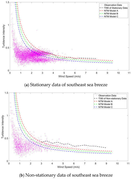
Figure 8.
Turbulence intensities of southeast sea breeze.
Although the NTM Models B and C also systematically underestimate turbulence intensity relative to field measurements, the 90th percentile values of the measured turbulence intensity are very close to those of NTM Model A. Specifically, at 4 m/s, the 90th percentile of the measured turbulence intensity is about 2% higher than Model A, while at 9 m/s, it is approximately 5% lower. This suggests that NTM Model A offers a more conservative and representative estimate of the upper turbulence intensity bound under the observed conditions, especially in the lower wind speed range where the deviation is slightly positive.
The results of the turbulence intensity of stationary southeast sea breeze are shown in Table 5.
Table 5.
Turbulence intensity of stationary data for southeast sea breeze.
3.3. Recalibration of Parameters for the NTM Model
3.3.1. Typhoon-Affected and Normal Sea Breeze
The Method of Bins is used again for the analysis of wind speed standard deviation. The values, computed from each 10 min segment, are reorganized into bins based on integer wind speed values. Subsequently, the mean and standard deviation of wind speed standard deviation within each bin are calculated based on the raw data.
According to Equations (3) and (4), both and are linear with mean wind speed . Therefore, a regression analysis was conducted on these data, and the resulting regression line is depicted in red, while the IEC regulation is represented by a blue dashed line. This approach aligns with established methodologies in wind turbulence analysis and IEC standard compliance assessments [25,26].
The values of and of typhoon-affected sea breeze, normalized by the reference turbulence intensity , are presented as black cycles in Figure 9a,b, respectively. The IEC Model A curve is represented by a blue dashed line and the linear regression line of observation data by a red line in Figure 9.
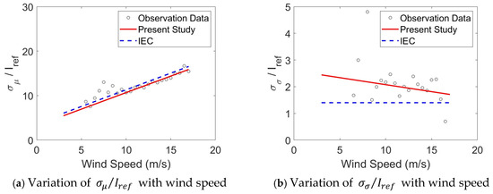
Figure 9.
Regression analysis of and for typhoon-affected sea breeze.
The values of and of normal sea breeze, normalized by the reference turbulence intensity , are presented in Figure 10a,b, respectively. The IEC Model B curve is represented by a blue dashed line and the linear regression line of observation data by a red line in Figure 10.
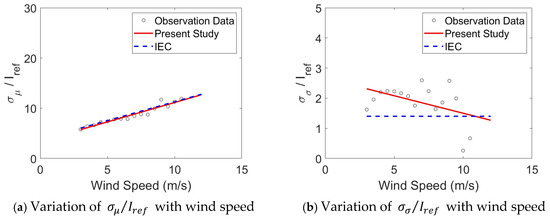
Figure 10.
Regression analysis of and for normal sea breeze.
As shown in Figure 9 and Figure 10, both typhoon-affected and normal sea breeze exhibit good agreement with the IEC standard model. Specifically, the turbulence intensity under typhoon-affected conditions is higher and closely aligns with NTM Model A ( = 0.16), which represents the highest turbulence level in the IEC specifications. To improve the modeling of standard deviation, the parameters and , as defined in Equation (3), have been identified as 0.743 and 3.241 through curve fitting, resulting in a significantly improved agreement with the measured data. The parameters and , as defined in Equation (4), have been identified as −0.052 and 2.599, respectively.
In contrast, the normal sea breeze corresponds more closely to NTM Model B ( = 0.14), characterized by lower turbulence intensity. The parameters and have been identified as 0.772 and 3.42 through curve fitting, also resulting in a significantly improved agreement with the measured data. The parameters and , as defined in Equation (4), have been identified as −0.116 and 2.661, respectively.
According to the regression analysis of variation of and , the NTM model parameters of the Pingtan observation campaign are determined using Equations (3) and (4). The results of the present study are shown in Table 6.
Table 6.
Proposed and IEC parameters.
3.3.2. Northeast and Southeast Sea Breeze
The values of and of northeast sea breeze, normalized by the reference turbulence intensity , are presented in Figure 11a,b, respectively. The IEC Model A curve is represented by a blue dashed line and the linear regression line of observation data by a red line in Figure 11.

Figure 11.
Regression analysis of and for northeast sea breeze.
Figure 11a illustrates the variation of with wind speed based on observational data, showing a linear increasing trend as wind speed rises. However, the observed values of are notably higher than those predicted by the IEC NTM model, indicating that the IEC model parameters do not accurately represent the observed data. To improve the modeling of standard deviation, the parameters and , as defined in Equation (3), have been identified as 1.648 and 1.074 through curve fitting, resulting in a significantly improved agreement with the measured data. Figure 11b illustrates the variation of with wind speed is a relatively flat trend, which is similar to IEC regulations. The parameters and , as defined in Equation (4), have been identified as 0.082 and 0.748, which closely align with the values recommended in IEC regulations, indicating consistency between the observed data and the standard model.
The values of and of southeast sea breeze, normalized by the reference turbulence intensity , are presented in Figure 12a,b, respectively. The IEC Model A curve is represented by a blue dashed line and the linear regression line of observation data by a red line in Figure 12.
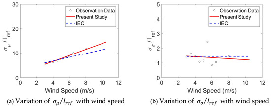
Figure 12.
Regression analysis of and for southeast sea breeze.
As shown in Figure 12, the results demonstrate a high level of consistency with the IEC standard model, indicating that the sea breeze from the southeast direction closely follows the turbulence characteristics defined by the IEC specifications. This good agreement suggests that the IEC model provides a reasonable representation of the southwest sea breeze regime.
The turbulence intensity of the sea breeze blowing from the northeast direction in the Huilai region of Guangdong Province is observed to be higher than that from the southeast direction. This difference can be primarily attributed to the influence of the Taiwan Strait. The northeast sea breeze traverses a longer and narrower passage over the Taiwan Strait, where complex land–sea interactions and topographical channeling effects enhance wind shear and turbulence generation. Additionally, the relatively cooler and more stable air masses over the strait promote stronger turbulence mixing as the airflow moves toward the coastal area. In contrast, the southeast sea breeze originates over the open South China Sea, where the airflow encounters fewer obstacles and a more uniform surface, resulting in comparatively lower turbulence intensity. Therefore, the unique geographic and meteorological conditions of the Taiwan Strait significantly contribute to the elevated turbulence intensity observed in the northeast sea breeze at Huilai.
According to the regression analysis of variation of and , the NTM model parameters of the Huilai observation campaign are determined using Equations (3) and (4). The results of present study are shown in Table 7.
Table 7.
Proposed and IEC parameters.
As previously discussed, these parameters for the mean value and standard deviation of of the NTM model are derived from a limited dataset of observational measurements. While multiple studies have confirmed the accuracy of the mean value of , recent observations indicate that the mean value parameters specified in IEC 61400-1 are consistently lower than those obtained from experimental data. This discrepancy highlights the need to reassess and update the representative standard deviation of wind speed in the next revision of IEC regulations to ensure better alignment with contemporary observational data and enhance the accuracy of turbulence modeling.
4. Conclusions
This study investigated the turbulence characteristics of offshore wind conditions at coastal sites in China, with a particular focus on the effects of sea breezes and typhoon events. By combining long-term observations with short-term typhoon-affected datasets, the analysis provided new insights into the applicability of IEC turbulence models in complex offshore environments. The findings reveal the limitations of the IEC NTM model in representing the turbulence characteristics of offshore wind conditions, particularly in coastal zones with pronounced sea breeze effects [27].
Two months of observations at Fujian included wind data influenced by Typhoon Haikui. Comparison of the results shows that both typhoon-affected and normal winds exhibit good agreement with the IEC NTM model, but they correspond to different model types: typhoon-affected winds align more closely with Model A, while normal winds are better represented by Model B. One-year field measurement at Guangdong demonstrated that the turbulence intensity of northeast sea breeze is approximately 30% higher than that predicted by the existing IEC NTM models. In contrast, the turbulence intensity of the southeast sea breeze is found to be close to the IEC model estimates.
This study provides advancements beyond previous research [16,17,18,19,20] in two key aspects. First, the use of high-frequency data from precision instruments allows for a more accurate determination of turbulence statistics. Second, it offers a novel comparative analysis of the turbulence characteristics of typhoon-affected versus normal conditions. The recalibrated model enhances wind turbine design by more accurately simulating the wind time series, which is the critical input for wind turbine simulations. This leads to more realistic predictions of operational and extreme loads, thereby improving the accuracy of subsequent stress analysis and structural optimization.
It is acknowledged that this study has certain limitations regarding the measurement sites. Firstly, the analysis is based on data from only two coastal sites, and the stations were located on the coast rather than offshore. Secondly, the typhoon-affected data are limited to a short period (6 days) and capture outer circulation effects rather than the typhoon core. Thirdly, the instrument measure the wind speed below typical wind turbine hubs height, which do not fully satisfy IEC requirements. Nevertheless, this study mainly focuses on methodology, aiming to show that turbulence models can be recalibrated using high-frequency wind data. To reduce site effects, the instruments were placed in elevated, open positions facing the sea.
Future research should focus on further refining and validating the proposed NTM parameters by incorporating longer-term field measurements from multiple offshore locations. Expanding the dataset will enhance the robustness of the new turbulence model and ensure its applicability across different coastal and deep-sea environments. Additionally, the dynamic response of wind turbines under different turbulence model should be investigated to quantify turbulence model’s direct impact on load prediction and design optimization.
Author Contributions
Conceptualization, S.D. and H.W.; methodology, S.D. and M.Y.; software, S.D. and Y.S.; validation S.D. and Y.S.; writing—original draft preparation, S.D.; writing—review and editing, S.D., Y.S. and Y.Z.; visualization, Y.Z.; supervision, J.-F.W.; funding acquisition, S.D. All authors have read and agreed to the published version of the manuscript.
Funding
This work was supported by the National Key R&D Program of China—Intergovernmental International Scientific and Technological Innovation and Cooperation Program (Grant No. 2023YFE0115400); the Shanghai Pujiang Program (Grant No. 22PJ1421200); the International Science and Technology Cooperation Project of Hubei Province (Grant No. 2024EHA030); and the Project of Shanghai Investigation, Design & Research Institute Co., Ltd. (Grant No. 2022QT(83)-035). The funders had no role in the design of the study; in the collection, analyses, or interpretation of data; in the writing of the manuscript; or in the decision to publish the results.
Data Availability Statement
The data presented in this study are not publicly available due to ownership and confidentiality restrictions.
Acknowledgments
The authors appreciate the valuable suggestions from Bert Sweetman at Texas A&M University, USA. The authors also appreciate the contributions from Caiyu Wang at Shanghai Investigation, Design, and Research Institute Co., Ltd., China, and Yan Nie at China Resources Power Technology Research Institute Company Limited, China.
Conflicts of Interest
Author Shu Dai and Yue Song were employed by the company Shanghai Investigation, Design, and Research Institute Co., Ltd. The remaining authors declare that the research was conducted in the absence of any commercial or financial relationships that could be construed as potential conflicts of interest.
References
- Shi, T.; Dai, S.; Tang, S.; Wang, H.; Song, Y.; Wen, J.F. Fatigue crack growth simulation of floating offshore wind turbine blades under non-Gaussian loading. Ocean Eng. 2025, 341, 122532. [Google Scholar] [CrossRef]
- IEC 61400-1:2019; Wind Turbines—Part 1: Design Requirements. International Electrotechnical Commission (IEC): Geneva, Switzerland, 2019.
- IEC 61400-12-1:2010; Wind Turbines—Part 12-1: Power Performance Measurements of Electricity Producing Wind Turbines. International Electrotechnical Commission (IEC): Geneva, Switzerland, 2010.
- Huang, Q.Q.; Cai, X.H.; Song, Y.; Kang, L. A numerical study of sea breeze and spatiotemporal variation in the coastal atmospheric boundary layer at Hainan Island, China. Bound.-Layer Meteorol. 2016, 161, 571–590. [Google Scholar] [CrossRef]
- Jiang, P.; Wen, Z.; Sha, W.; Chen, G. Interaction between turbulent flow and sea breeze front over urban-like coast in large-eddy simulation. J. Geophys. Res. Atmos. 2017, 122, 3421–3438. [Google Scholar] [CrossRef]
- Soares, P.M.M.; Lima, D.C.A. Global offshore wind energy resources using the new ERA-5 reanalysis. Environ. Res. Lett. 2020, 15, 1040a2. [Google Scholar] [CrossRef]
- Sathe, A.; Mann, J.; Gottschall, J.; Courtney, M.S. Can wind lidars measure turbulence? J. Atmos. Ocean. Technol. 2011, 28, 853–868. [Google Scholar] [CrossRef]
- Finocchio, P.M.; Biernat, K.A.; Doyle, J.D.; Reynolds, C.A. The influence of soil moisture on the sea-breeze circulation and the marine atmospheric boundary layer in idealized simulations. Mon. Weather. Rev. 2025, 153, 1651–1669. [Google Scholar] [CrossRef]
- Liu, L.; Hu, F. Finescale clusterization intermittency of turbulence in the atmospheric boundary layer. J. Atmos. Sci. 2020, 77, 2375–2392. [Google Scholar] [CrossRef]
- Yang, X.; Yang, Y.; Li, M.; Wang, P. Effects of free-stream turbulence on non-Gaussian characteristics of fluctuating wind pressures on a 5:1 rectangular cylinder. J. Wind. Eng. Ind. Aerodyn. 2021, 217, 104759. [Google Scholar] [CrossRef]
- Ha, Y.; Ahn, H.; Park, S.; Park, J.; Kim, K. Development of Hybrid Model Test Technique for Performance Evaluation of a 10 MW Class Floating Offshore Wind Turbine Considering Asymmetrical Thrust. Ocean. Eng. 2023, 272, 113783. [Google Scholar] [CrossRef]
- Wang, X.; Huang, P.; Yu, X.-F.; Wang, X.-R.; Liu, H.-M. Near ground wind characteristics during typhoon Meari: Turbulence intensities, gust factors, and peak factors. J. Cent. South Univ. 2017, 24, 2421–2430. [Google Scholar] [CrossRef]
- Duan, Z.; Yao, X.; Li, Y.; Lei, X.; Fang, P.; Zhao, B. Investigation of turbulent momentum flux in the typhoon boundary layer. J. Geophys. Res. Ocean. 2017, 122, 2259–2268. [Google Scholar] [CrossRef]
- Lin, L.; Chen, K.; Xia, D.; Wang, H.; Hu, H.; He, F. Analysis on the wind characteristics under typhoon climate at the southeast coast of China. J. Wind. Eng. Ind. Aerodyn. 2018, 182, 37–48. [Google Scholar] [CrossRef]
- Qin, Z.; Xia, D.; Dai, L.; Zheng, Q.; Lin, L. Investigations on wind characteristics for typhoon and monsoon wind speeds based on both stationary and non-stationary models. Atmosphere 2022, 13, 178. [Google Scholar] [CrossRef]
- Ishihara, T.; Yamaguchi, A.; Sarwar, M.W. A Study of the Normal Turbulence Model in IEC 61400-1. Wind. Eng. 2012, 36, 759–766. [Google Scholar] [CrossRef]
- Leu, T.S.; Yo, J.M.; Tsai, Y.T.; Miau, J.J.; Wang, T.C.; Tseng, C.C. Assessment of IEC 61400-1 normal turbulence model for wind conditions in Taiwan west coast areas. Int. J. Mod. Phys. Conf. Ser. 2014, 34, 1460382. [Google Scholar] [CrossRef]
- Dai, S.; Zheng, Y.; Song, Y.; Yang, W.; Shi, Y.; Wang, H.; Wen, J.F. Observation and Analysis of Sea Breeze Characteristics Over the Coastal Region of Shantou, China. In Proceedings of the ISOPE International Ocean and Polar Engineering Conference, Goyang, Republic of Korea, 1–6 June 2025; ISOPE: Cupertino, CA, USA; p. ISOPE–I. [Google Scholar]
- Dai, S.; Sweetman, B. Physics-based recalibration method of cup anemometers. Flow Meas. Meas. Meas. Instrum. 2023, 91, 102343. [Google Scholar] [CrossRef]
- Cheng, K.-S.; Ho, C.-Y.; Teng, J.-H. Wind characteristics in the Taiwan Strait: A case study of the first offshore wind farm in Taiwan. Energies 2020, 13, 6492. [Google Scholar] [CrossRef]
- Vahidi, D.; Porte-Agel, F. Influence of incoming turbulent scales on the wind turbine wake: A large-eddy simulation study. Phys. Fluids 2024, 36, 095177. [Google Scholar] [CrossRef]
- Ren, L.; Zhang, W.; Wang, Y.; Wang, H.; Yang, H.; Yao, P. Distribution characteristics and assessment of wind energy resources in the coastal areas of Guangdong. Sustain. Energy Technol. Assess. 2024, 59, 103249. [Google Scholar] [CrossRef]
- Chien, W.T.K.; Yang, S.F. Using reverse arrangement test to detect non-monotonic trends for semiconductor manufacturing and reliability tests. Int. J. Reliab. Qual. Saf. Eng. 2008, 15, 497–514. [Google Scholar] [CrossRef]
- Jeans, G. Converging profile relationships for offshore wind speed and turbulence intensity. Wind. Energy Sci. 2024, 9, 2001–2024. [Google Scholar] [CrossRef]
- Veers, P.S. Three-Dimensional Wind Simulation; Sandia National Laboratories: Albuquerque, NM, USA; Livermore, CA, USA, 1988; No. SAND88-0152. [Google Scholar]
- Kelley, N.D. Turbulence-Turbine Interaction: The Basis For the Development of the TurbSim Stochastic Simulator; National Renewable Energy Laboratory: Golden, CO, USA, 2004; No. NREL/TP-500-41137. [Google Scholar]
- Hevia-Koch, P.; Jacobsen, H.K. Comparing offshore and onshore wind development considering acceptance costs. Energy Policy 2019, 132, 9–19. [Google Scholar] [CrossRef]
Disclaimer/Publisher’s Note: The statements, opinions and data contained in all publications are solely those of the individual author(s) and contributor(s) and not of MDPI and/or the editor(s). MDPI and/or the editor(s) disclaim responsibility for any injury to people or property resulting from any ideas, methods, instructions or products referred to in the content. |
© 2025 by the authors. Licensee MDPI, Basel, Switzerland. This article is an open access article distributed under the terms and conditions of the Creative Commons Attribution (CC BY) license (https://creativecommons.org/licenses/by/4.0/).