Article

LSTM-Based Predefined-Time Model Predictive Tracking Control for Unmanned Surface Vehicles with Disturbance and Actuator Faults

Marine Electrical Engineering College, Dalian Maritime University, Dalian 116026, China
*
Author to whom correspondence should be addressed.
J. Mar. Sci. Eng. 2025, 13(10), 1914; https://doi.org/10.3390/jmse13101914
Submission received: 12 September 2025 / Revised: 29 September 2025 / Accepted: 3 October 2025 / Published: 5 October 2025
(This article belongs to the Special Issue The Control and Navigation of Autonomous Surface Vehicles)

Abstract

Predefined-time control has been extensively implemented in marine control systems due to its capability to enhance transient performance and achieve superior control specifications. However, inaccurate control execution resulting from faulty actuators can compromise this control strategy and critically undermine system performance. To address this challenge, this paper propose a predefined-time model predictive fault-tolerant control strategy for unmanned surface vessels (USVs) while considering actuator failures and ocean disturbances. Firstly, a novel predefined-time model predictive control (PTMPC) strategy is designed by incorporating contraction constraints derived from an auxiliary predefined-time control system into the proposed optimization framework. This ensures that the resulting control variables guarantee predefined-time convergence of tracking errors when applied to the USV system. Furthermore, a long short-term memory-based neural network for disturbance prediction is integrated into the control strategy, leveraging its exceptional capability in modeling temporal sequences to achieve accurate forecasting of ocean disturbances. Thirdly, the proposed control scheme utilizes its integrated fault observation mechanism to actively compensate for actuator failures through real-time fault estimation, ensuring predefined-time convergence performance while providing rigorous guarantees of closed-loop stability and feasibility. Finally, simulation results demonstrate the efficacy and superiority of the proposed algorithm.

1. Introduction

In recent decades, the rapid advancement of navigation and automation technologies has spurred considerable research interest in unmanned surface vessels (USVs), owing to their critical functions across diverse marine applications including environmental monitoring, resource exploration, and naval defense [1,2,3]. Among various control objectives proposed for these missions, trajectory tracking represents a widely adopted strategy for USVs, enabling precise adherence to stringent spatiotemporal paths. However, practical implementation confronts significant obstacles in achieving precise tracking control due to the inherent nonlinear dynamics of USVs and the operational complexity of maritime environments [4,5]. This necessitates the development of advanced nonlinear control strategies to reduce disturbance vulnerability, enhance fault tolerance, and improve mission efficiency. Motivated by practical requirements, diverse nonlinear control methodologies such as sliding mode control [6], backstepping control [7], adaptive control [8], neural network control [9], and fuzzy control [10] have been successfully employed for trajectory tracking of USVs. However, these approaches [6,7,8,9,10] frequently overlook inherent physical system constraints. For marine vessels, control inputs must enforce practical limitations on thrust generation, making the explicit incorporation of input constraints imperative in control strategy design [11].
In this regard, model predictive control (MPC) presents a promising solution by providing a systematic framework for handling constraints while ensuring optimal performance relative to specified criteria [12]. Conventional MPC strategies necessitate terminal sets and guarantee stability by enforcing state convergence into these sets within the prediction horizon through optimized decision variables [13]. However, for strongly coupled nonlinear USV control systems, the selection of appropriate terminal sets and constraints becomes particularly challenging, significantly impeding the practical implementation of MPC in marine applications [14]. Fortunately, Lyapunov-based MPC (LMPC) eliminates terminal set and constrant dependencies through an auxiliary Lyapunov-function-based controller, ensuring stability and feasibility while facilitating practical deployment in marine systems [15,16]. Nevertheless, persistent environmental perturbations, amplified by complex hydrodynamic interactions, pose a significant threat to the stability of USVs [11]. To mitigate these effects, of particular relevance to marine applications, neural network-based disturbance observers have emerged as a promising paradigm due to their inherent capability to accurately approximate complex nonlinear dynamics [17,18]. Among them, long short-term memory (LSTM) networks, with their sophisticated gating mechanisms, demonstrate exceptional proficiency in identifying and capturing long-range temporal dependencies—a critical advantage for predicting marine disturbances such as wind, waves, and ocean currents, which often exhibit strong temporal correlations and non-stationary behavior [19]. Unlike conventional observers that rely on simplified physical models, LSTM-based observers can learn directly from historical system data, effectively encoding the underlying temporal patterns of time-varying marine disturbances without requiring explicit mathematical models [20]. This capability makes them particularly suitable for marine environments where disturbances are repetitive yet influenced by long-term historical states. Consequently, the integration of an LSTM-based disturbance observer into the LMPC framework offers a principled and systematic methodology to enhance prediction accuracy and robustness in USV trajectory tracking, enabling more anticipative and adaptive control under realistic sea conditions.
Furthermore, the extensive application of USVs hinges upon their operational reliability in diverse and complex scenarios. Thrusters serve as critical propulsion components for USVs [21]. However, these actuators are susceptible to performance degradation due to environmental factors (e.g., seawater corrosion) or aging effects, potentially leading to failures such as mechanical deformation and drive motor overload [22]. Under such fault conditions, conventional control strategies may prove inadequate. Consequently, for safety-critical systems like USVs, the implementation of fault-tolerant control is of paramount importance to enhance operational reliability and ensure system integrity [23]. Reference [23] introduced an iterative adaptive observer utilizing neural network techniques to provide precise estimates of sensor failures. Reference [24] developed a nonlinear disturbance observer to estimate the aggregate disturbances, encompassing both external environmental influences and actuator failures, and demonstrated that the closed-loop signals are uniformly ultimately bounded. Nevertheless, actuator failures induce significant performance deterioration and control efficiency reduction, mandating fault-tolerant control architectures with rigorous transient response specifications to ensure operational integrity and achieve system control requirements [25]. Currently, with the rapid advancement of control theory, finite-time and fixed-time control strategies have been recognized as highly effective approaches for optimizing system convergence time [26,27]. Despite their significant contributions to enhancing control performance, these methods exhibit certain limitations: finite-time control is inherently dependent on initial conditions, making it difficult to determine the exact settling time when the system’s initial state is unknown [28]. Although fixed-time control eliminates the reliance on initial conditions, its convergence time cannot be explicitly specified by the designer, which restricts its applicability in scenarios requiring precise timing guarantees [29]. In contrast, the proposed predefined-time control strategy effectively overcomes these drawbacks. Predefined-time control allows the convergence time to be set arbitrarily by the control parameters in advance, ensuring that the system states reach stability within a user-defined duration [30]. This capability is particularly critical in the context of fault-tolerant and safety-critical control systems, where timely response is essential to maintain system integrity under adverse conditions. For USVs operating in uncertain marine environments, the ability to predefine the convergence time provides a crucial guarantee for rapid fault recovery and safe navigation, especially in the presence of actuator failures or sudden disturbances [31]. By integrating predefined-time stability with fault-tolerant control design, this approach not only enhances the robustness of the system but also offers a predictable and verifiable safety assurance, which is a fundamental requirement for modern autonomous marine systems. However, considering the diversity and uncertainty of the faults, achieving the predefined time control for the USV control system remains a significant challenge.
Building upon this analysis, this paper proposes a novel predefined-time MPC (PTMPC) framework to address external disturbances and actuator failures in USVs. Significantly, by integrating a predefined-time auxiliary control system with an LSTM neural network into the MPC architecture, the framework guarantees predefined time convergence of tracking errors under both disturbances and actuator faults. Concurrently, it leverages the inherent optimization capabilities of MPC to refine control inputs, thereby minimizing resource consumption while maintaining stability guarantees. The principal contributions of this work are as follows:
(1)
A novel model predictive optimization control framework has been developed by incorporating contraction constraints derived from a predefined-time Lyapunov function into the optimization problem. This formulation ensures that the resulting control inputs guarantee predefined-time convergence of tracking errors while substantially enhancing the control performance of MPC.
(2)
Leveraging the inherent capability of LSTM neural networks to model temporal dependencies in sequential data, oceanic disturbances can be accurately forecasted. Integrating these predictions into the control strategy substantially improves system robustness, enabling reliable operation in highly dynamic marine environments.
(3)
By integrating a predefined-time fault observer into the model predictive control architecture, precise fault information can be ascertained within a predefined-time interval. This strategic incorporation of temporal fault observation enhances the system’s transient performance while ensuring robust fault-tolerant capabilities, thereby extending operational viability across a broader spectrum of fault scenarios.
The rest of this article is organized as follows: The problem description and the ship and fault model are provided in Section 2. A predefined-time auxiliary control system integrating an LSTM neural network observer and a predefined-time fault observer is designed in Section 3. Model predictive optimization problem construction and proof of stability and feasibility are presented in Section 4. Simulation studies are demonstrated in Section 6. Finally, Section 7 concludes this article.
Notation: We write R for the set of real numbers, R n for the space of n-dimensional real column vectors, and R m × n for the space of m × n real matrices. For a matrix A , A denotes the induced Euclidean norm, and A T denotes the transpose of A . Let diag ( x 1 , , x n ) be the diagonal matrix with diagonal entries x 1 , , x n . For x = [ x 1 , , x n ] R n , define sig r ( x ) : = [ | x 1 | r sgn ( x 1 ) , , | x n | r sgn ( x n ) ] , where sgn ( · ) is the sign function.

2. Problem Statement

2.1. USVs Model

This study investigates three degrees of freedom horizontal motion in USVs under the conventional assumption of minimal roll and pitch angles [32]. As shown in Figure 1, a body-fixed reference frame is defined with the center of gravity as its origin to describe vessel motion. The kinematic formulation characterizes the displacement between this body frame and an Earth-fixed inertial frame. After eliminating heave, roll and pitch components, the analysis considers a homogeneous group of unmanned surface vessels with identical dynamic properties. The derived kinematic relationships are presented as follows:
η ˙ = R ( ψ ) ϑ ,
where η = x , y , ψ T denotes the position coordinate of x , y T and heading angle ψ of USVs in the earth-fixed inertial frame; and ϑ = u , v , r T denotes the velocity vector in the body-fixed coordinate frame, u and v are velocities of the vehicle in the surge and sway, r is the yaw velocity of the USV. R ( ψ ) is the rotation matrix in yaw and is denoted as follows:
R ( ψ ) = cos ( ψ ) sin ( ψ ) 0 sin ( ψ ) cos ( ψ ) 0 0 0 1 ,
with the following properties:
R ˙ ( ψ ) = R ( ψ ) S ( r ) ,
R T ( ψ ) R ( ψ ) = I 3 × 3 , ψ 0 , 2 π ,
where
S ( r ) = 0 r 0 r 0 0 0 0 0 .
The dynamic equation is formulated by incorporating the USV matrices M , C ( ϑ ) , and D ( ϑ ) within the body-fixed coordinate system, in accordance with Newton’s laws [32]
M ϑ ˙ + C ( ϑ ) ϑ + D ( ϑ ) ϑ = τ + τ ω ,
where
M = m 11 0 0 0 m 22 0 0 0 m 33
represents the inertia matrix including the added mass;
C ( ϑ ) = 0 0 m 22 v 0 0 m 11 u m 22 v m 11 u 0
denotes the Coriolis and centripetal matrix and
D ( ϑ ) = d 11 + d n 11 | u | 0 0 0 d 22 + d n 22 | v | 0 0 0 d 33 + d n 33 | r |
is the damping matrix. τ = τ 1 , τ 2 , τ 3 T is the control input vector of USVs, τ ω denotes external disturbances (induced by winds, waves and strong currents, etc).
Consider the coordinate transformation given by
ω = R ( ψ ) ϑ ,
where ω = ω u , ω v , ω r T . Together with the kinematic equation in (1) and the dynamic equation in (5) and properties of R ( ψ ) , the transformed dynamics become
x ˙ = ω h ( η , ω ) + R M 1 τ + d ω ,
where d ω = R M 1 τ ω . x = col ( η , ω ) is the state vector of USVs, and h ( η , ω ) = S ω R M 1 ( C + D ) R T ω .

2.2. The Fault Model of USVs

Considering the comprehensive thruster fault model in [3], the control input τ f ( t ) under the actuator failure is expressed as follows:
τ f ( t ) = Θ τ ( t ) + τ s ,
Θ = diag ( Θ 1 , Θ 2 , Θ 3 ) are the failure factor, which denotes a diagonal semi-positive-definite weighting matrix that characterizes the effectiveness of the thrusters and 0 < Θ j 1 . τ s = u s 1 , u s 2 , u s 3 T denotes as corresponding bias fault. ϕ j and u s j are unknown constants, where j = 1 , 2 , 3 .
Remark 1. 
The proposed fault model comprehensively captures realistic actuator failure modes in unmanned surface vessels through multiplicative Θ and additive bias fault components τ s . Multiplicative faults typically originate from mechanical degradation and electrical component aging, while additive faults arise from installation misalignment or persistent mechanical deviations. This integrated framework, incorporating both additive and multiplicative fault types, enables representation of diverse failure scenarios and is widely adopted in fault-tolerant control architectures for autonomous systems.
Considering the actuator saturation and fault, Equation (10) can be reformulated as follows:
x ˙ = ω h ( η , ω ) + R M 1 τ f + d ω = ω h ( η , ω ) + R M 1 Θ τ + R M 1 τ s + d ω = f ( x , τ ) .
Assumption 1. 
The external environmental disturbances suffered by USVs are bounded and slowly time-varying, i.e., | d ˙ ω j | δ 1 j , | d ω j | δ 2 j , j = 1 , 2 , 3 . δ 1 = δ 11 , δ 12 , δ 13 T and δ 2 = δ 21 , δ 22 , δ 23 T are the positive vectors.
Assumption 2. 
The bias fault τ s are bounded in such that | τ s j | τ ¯ s . The failure factor Θ = diag ( Θ 1 , Θ 2 , Θ 3 ) satisfies
0 Θ ̲ Θ i Θ ¯ 1
where the lower bound Θ ̲ and upper bound Θ ¯ are positive constants.
Remark 2. 
In practical marine environments, external disturbances acting on vessels primarily originate from physical environmental factors such as wind, waves, and currents. Given that these natural phenomena operate under finite energy and power constraints, Assumption 1 postulating bounded magnitude and rate of marine disturbances remains physically justified. Furthermore, Assumption 2 of known bounds for multiplicative fault factors in fault-tolerant control is widely applied in the field of maritime control systems. On one hand, in many practical engineering applications, particularly those involving high-reliability control systems, the upper and lower bounds of the fault factors can often be estimated using prior knowledge, such as historical fault data and the physical characteristics of the actuators. On the other hand, with the continuous advancement of sensor technologies and algorithms in intelligent vessels, it becomes feasible to roughly estimate the type and extent of actuator faults, thereby determining the bounds of the fault factors. Simultaneously, considering the inherent physical saturation characteristics of USV thrusters, the assumption of bounded actuator bias faults is equally well-founded.

2.3. Control Objective

The control objective of this study is to develop a predefined-time model predictive fault-tolerant control strategy incorporating LSTM neural networks. This framework achieves the tracking errors within the invariant set X , as defined in (50) converge to a neighborhood of the origin within a predefined time while compensating for external disturbances and actuator faults, and while simultaneously optimizing performance metrics and control efficacy. The system architecture is illustrated in Figure 2.

3. Design of the Auxiliary Control System

3.1. LSTM Network

MPC leverages its formidable optimization capabilities to generate high performance control input signals, making it widely applicable in advanced control systems. However, conventional MPC strategies depend critically on precise system models and real-time state measurements to dynamically optimize system behavior. In complex maritime environments, persistent oceanic disturbances, including wind, waves, and currents continuously affect vessel dynamics. Consequently, obtaining accurate system models for unmanned surface vehicles under such exogenous disturbances remains a significant challenge.
Neural networks provide a powerful methodology for learning and identifying unknown marine disturbances by leveraging their exceptional capability to capture input-output characteristics of nonlinear functions. Through historical data training, time-series prediction models such as recurrent neural networks can effectively learn the dynamic patterns of oceanic disturbances under evolving environmental conditions. Although recurrent neural networks capture temporal dependencies, they suffer from gradient explosion and vanishing gradient problems due to accumulated weights within sliding windows. Long Short-Term Memory networks address these limitations through specialized memory cells that extract sequential features from time-series data, enabling accurate long-term predictions. Combined with their computational efficiency and generalization capability, LSTMs represent an ideal choice for marine disturbance prediction and control tasks addressed in this work.
In the LSTM-based marine disturbance prediction strategy, we focus on the primary disturbance sources encountered by USVs such as ocean winds and waves. These external environmental factors significantly influence the vessel’s motion stability through complex hydrodynamic interactions. To more accurately characterize marine disturbances, this study employs multisource sensor data to construct the input features for the neural network, which include the vessel’s position and velocity, real-time wind speed, water flow velocity, and the thrust provided by the propulsion system. Additionally, the actual marine disturbance values are derived by solving the vessel model (10), serving as supervisory signals to form the training dataset for the LSTM disturbance observer, allowing it to learn the mapping relationship between inputs and outputs.
Specifically, the LSTM architecture employs three fundamental gating mechanisms: an input gate, an output gate, and a forget gate. The forget gate determines which information to retain or discard within the cell state via a sigmoid activation function σ , expressed mathematically as follows:
f t = σ W h f h t 1 + W u f u t + b f
where h t 1 denotes the previous hidden state, u t represents the current input vector, and σ ( · ) is the sigmoid activation function, with output ranges of [ 1 , 1 ] . The weight matrices W h f and W u f correspond to the hidden and input connections, respectively, while b f denotes the bias term.
Then it is necessary to determine which new information needs to be added to the unit status. The input gate is used to determine which information needs to be updated. Then, a t a n h function will be used to obtain the new candidate unit information, which may be updated into the unit state. The specific calculation method is as follows:
i t = σ ( W h i ζ t h t 1 + W u i u t + b i ) ,
c ˜ t = tanh W h c ζ t h t 1 + W u c u t + b c
where ⊗ means element-wise multiplication. c ˜ t is the candidate memory state, the weight matrices W h i , W h c , and W u i correspond to the hidden and input connections, respectively, while b i and b c denote the bias term. Notation t a n h ( · ) represent the hyperbolic tangent function, with output ranges of [ 1 , 1 ] .
Subsequently, the existing cell state information undergoes selective updating through a structured modulation process. During this phase, the forget gate selectively eliminates obsolete information, while the input gate strategically incorporates relevant data from candidate cell states, collectively generating an updated cell representation. This procedure is mathematically represented as follows:
c t = f t c t 1 + i t c ˜ t
where c t denotes the cell state. After updating the cell state, the output gate needs to process the sum of the inputs to describe the output cell state. Then, the output cell state is processed to obtain the network output y t , and its calculation is as follows:
o t = σ W h o h t 1 + W u o u t + b o
h t = o t tanh c t
y t = σ * W y h t + b y
where σ * ( · ) is the element-wise activation function, and W h o , W u o , and W y are the weight matrix and b o and b y are the bias terms.
Let T be the hypothesis class of machine learning models mapping u = { u 1 , , u z } R d u × z to y R d y and let G be the associated loss function class defined as follows:
G = { g : u , y ^ L B ( u ) , y ^ = L y , y ^ , B B }
where y ^ is the output vector of the machine learning model, and z is a positive integer, representing the sliding window of network, respectively. The loss function L B ( u ) , y ^ = L y , y ^ is explicitly defined as the squared Euclidean distance between the true output y and the predicted output y ^ , i.e., L y , y ^ = i = 1 d y ( y i y ^ i ) 2 . d u and d y correspond to the dimensions of u and y . Then, according to [33], given a dataset S = { ( u 1 , y 1 ) , , ( u m , y m ) } of m i.i.d. samples, and assuming the loss g G is bounded, the following inequality holds with probability at least 1 δ for all g G :
E [ L ( y , y ^ ) ] 1 m i = 1 m L ( y i , y ^ i ) + 2 R s ( G ) + 3 log 2 ( 2 δ ) 2 m
where E [ L ( y , y ^ ) ] expresses the mathematical expectation of L ( y i , y ^ i ) , y i represents the output corresponding to the i th sample. u i = { u 1 i , , u z i } R d u × z . As shown in Equation (21), the upper bound of the generalization error is governed by the training error 1 m i = 1 m L ( y i , y ^ i ) , the Rademacher complexity R s ( G ) , and a function of m and δ . The empirical Rademacher complexity is defined as follows:
R s ( G ) = E sup g G 1 m i = 1 m ϵ i g ( u i , y ^ i ) = E sup B T 1 m i = 1 m ϵ i L ( B ( u i ) , y ^ i )
ϵ i represents a sequence of independent and identically distributed Rademacher random variables, with P ( ϵ i = 1 ) = P ( ϵ i = 1 ) = 1 2 .
Furthermore, according to the above description, the LSTM network trained on m samples achieves, with confidence at least 1 δ , an upper bound for the prediction error at time t k between the estimated disturbance d ^ ω ( t k ) and true disturbance d ω ( t k ) :
L d ω ( t k ) , d ^ ω ( t k ) = d ω ( t k ) d ^ ω ( t k ) 2 2 1 m i = 1 m L d ω i , d ^ ω i + 2 R s ( G ) + 3 log 2 2 δ 2 m W
W is a constant value, intrinsically linked to the training dataset and the associated confidence level, d ^ ω represents the forecasting discrepancy of oceanic disturbances derived from the LSTM-based estimation framework for USVs.
Remark 3. 
The proposed Equation (23) establishes the generalization error bound of the LSTM architecture, explicitly relating it to empirical training error, Rademacher complexity, dataset cardinality, and statistical confidence levels. Equation (23) demonstrates that systematic augmentation of training samples or improvement of training accuracy effectively tightens this bound, ensuring compliance with rigorous closed-loop stability guarantees.
Remark 4. 
LSTM network is selected as the predictive model for marine disturbance observation due to its superior ability to capture long-term temporal dependencies, which is essential for time series forecasting tasks like marine disturbance prediction. Unlike convolutional neural networks [34], which focus on spatial features, LSTM excels in modeling sequential data with strong temporal dependencies. Additionally, while gated recurrent units [35] offers faster training, LSTM’s more refined gating mechanisms allow for better handling of long sequences. Compared to linear models such as adaptive filters, LSTM’s nonlinear nature makes it more effective in capturing the complex, non-stationary dynamics of marine disturbances caused by environmental factors like wind, waves, and currents. Thus, LSTM is deemed the suitable choice for this task.

3.2. Predefined-Time Fault Observer

In this section, the predefined-time fault observer is designed for the estimates of fault information in (11).
The estimation errors for the variables in the observer system are defined as the difference between the true values and their respective estimates. Specifically, for the unknown Θ and τ s , the estimation errors are as follows:
Define the estimation errors of observer ω ˜ = ω ω ^ , Θ ˜ = Θ Θ ^ , and τ ˜ s = τ s τ ^ s , where ω ^ = ω ^ u , ω ^ v , ω ^ r T , Θ ^ = diag ( Θ ^ 1 , Θ ^ 2 , Θ ^ 3 ) and τ ^ s = τ ^ s 1 , τ ^ s 2 , τ ^ s 3 T are the estimations of ω , Θ and τ s in the observer system, respectively.
Then, the predefined-time fault observer for USVs is designed as
ω ^ ˙ = d ^ ω + h ( η , ω ) + R M 1 ( Θ ^ τ + τ ^ s ) + π q 1 T c sig 1 + q 1 ( ω ˜ ) + π q 1 T c sig 1 q 1 ( ω ˜ ) + W sign ( ω ˜ ) , θ ^ ˙ = ( R M 1 T ) T ω ˜ + 2 π q 1 T c sign ( θ ^ ) , τ ^ ˙ s = ( ω ˜ T R M 1 ) T = ( M 1 ) T R T ω ˜ ,
where θ ˜ = Θ ˜ I 3 × 1 = θ ˜ 1 , θ ˜ 2 , θ ˜ 3 T , T = diag ( τ 1 , τ 2 , τ 3 ) , q 1 ( 0 , 1 ) , T c represents the designed observation time.
Consider the Lyapunov function candidate
V 1 = 1 2 ω ˜ T ω ˜ + 1 2 θ ˜ T θ ˜ + 1 2 τ ˜ s T τ ˜ s ,
and incorporating Equations (12) and (24), the time derivative of V 1 is as follows:
V ˙ 1 = ω ˜ T ω ˜ ˙ + θ ˜ T θ ˜ ˙ + τ ˜ s T τ ˜ ˙ s = ω ˜ T ( R M 1 Θ ˜ τ + R M 1 τ ˜ s + d ˜ ω π q 1 T c sig 1 + q 1 ( ω ˜ ) π q 1 T c sig 1 q 1 ( ω ˜ ) W sign ( ω ˜ ) ) + θ ˜ T θ ˜ ˙ + τ ˜ s T τ ˜ ˙ s = ω ˜ T ( R M 1 T θ ˜ + R M 1 τ ˜ s + d ˜ ω π q 1 T c sig 1 + q 1 ( ω ˜ ) π q 1 T c sig 1 q 1 ( ω ˜ ) W sign ( ω ˜ ) ) θ ˜ T ( R M 1 T ) T ω ˜ π q 1 T c θ ˜ T sign ( θ ^ ) π q 1 T c θ ˜ T sign ( θ ^ ) τ ˜ s T ( M 1 ) T R T ω ˜
Given that 0 θ i 1 , it follows that θ ^ i 0 and 0 θ ˜ i 1 during the observation procedure. Consequently, 0 θ ˜ i 1 q 1 1 and 0 θ ˜ i 1 + q 1 1 hold. And combining ω ˜ T W sign ( ω ˜ ) = W i = 1 3 | ω ˜ i | ω ˜ T d ˜ ω , Equation (26) can be reformulated as
V ˙ 1 π q 1 T c ( ω ˜ T ω ˜ ) 1 + q 1 2 π q 1 T c ( ω ˜ T ω ˜ ) 1 q 1 2 π q 1 T c ( θ ˜ T θ ˜ ) 1 + q 1 2 π q 1 T c ( θ ˜ T θ ˜ ) 1 q 1 2 π q 1 T c ( V 1 1 + q 1 2 + V 1 1 q 1 2 ) + C 1
where C 1 = τ ¯ s 2 2 + q 1 + τ ¯ s 2 2 q 1 .
According to [36], the observation errors θ ˜ and τ ˜ s will converge to the residual set
ω ˜ , θ ˜ , τ ¯ s | V 1 min 2 q 1 T c C 1 π 2 2 + q 1 , 2 q 1 T c C 1 π 2 2 q 1 = χ ¯ 1
in a predefined time, the settling time T p satisfies T p 2 T c , χ ¯ 1 is a positive constant.

4. Main Results

In this section, we have designed an auxiliary control system based on a predefined-time sliding mode control law, and proved that the designed control strategy can ensure that the tracking error converges to the neighborhood of the origin within the predefined time.
Define the error vectors e 1 = ω ω d = e 11 , e 12 , e 13 T . We can use the nonlinear terminal sliding surfaces s is propsed as follows:
s = e ˙ 1 + k 1 e 1 1 + p 2 + k ( e 1 ) e 1 1 p 2 ,
where k 1 = π q 2 T r I 3 × 3 denotes positive definite symmetric matrices composed of positive real numbers. k ( e 1 ) = diag ( k 21 ( e 11 ) , k 22 ( e 12 ) , k 23 ( e 13 ) ) , 0 > q 2 > 0 . k 2 j ( e 1 j ) are designed as follows:
k 2 j ( e 1 j ) = π q 2 T r , | e 1 j | > ε , 0 , otherwise .
where k 1 j , k 2 j are positive real numbers, j = 1 , 2 , 3 , ε > 0 is a small constant parameter.
According to (10) and (29), it can be further obtained:
s ˙ = R M 1 ( θ τ + τ s + M R T h ( η , ω ) + d ω ) ω ˙ d + ( 1 + p 2 ) k 1 e 1 p 2 e ˙ 1 + α 1 ,
where α 1 = α 11 , α 12 , α 13 T is designed as follows:
α 1 j = π q 2 T r ( 1 p 2 ) e 1 j p 2 e ˙ 1 j , | e 1 j | > ε 0 , otherwise
To achieve the tracking error converge in a predefined time, the control law τ a is designed as follows:
τ a = θ ^ 1 M R T ( h ( η , ω ) R M 1 τ ^ s R M 1 d ^ ω + ω ˙ d ( 1 + p 2 ) k 1 e 1 p 2 e ˙ 1 α 1 k 3 s 1 + p 2 k 4 s 1 p 2 e 1 ) ,
where k 3 = π q 2 T r I 3 × 3 and k 4 = π q 2 T r I 3 × 3 denote positive definite symmetric matrices composed of positive real numbers k 3 j and k 4 j .
Remark 5. 
Note that the auxiliary controller τ a given term α 1 , that causes singularity problem when e 1 j 0 . To reduce the chattering phenomenon, the following term k ( e 1 j ) can be adopted to replace the singular term. This strategy ensures that α 1 can be constrained within a bounded range.
Theorem 1. 
Suppose Assumptions 1 and 2 hold. Consider the USVs system (10), the control input u a designed in (33) guarantees that the tracking errors e 1 within set X can convergence to the neighbor of the origin within a predefined time, with the settling time bounded by 2 2 T r + 2 T c , where T r and T c represent the observation time of the predefined fault observers and the error convergence time as defined in the sliding mode controller, X is defined in Equation (50).
Proof. 
Consider the function V 1 = 1 2 e 1 T e 1 , take the derivative of V 1 , we get
V ˙ 1 = e 1 T e ˙ 1 = e 1 T ( s k 1 e 1 1 + p 2 k ( e 1 ) e 1 1 p 2 ) = e 1 T s e 1 T k 1 e 1 1 + p 2 e 1 T k ( e 1 ) e 1 1 p 2 .
For the function
V 2 = V 1 + 1 2 s T s ,
according (31) and (34), its time derivative becomes
V ˙ 2 = V ˙ 1 + s T s ˙ = e 1 T s e 1 T k 1 e 1 1 + p 2 e 1 T k ( e 1 ) e 1 1 p 2 + s T ( R M 1 ( θ ^ τ a + θ ˜ τ a + τ ^ s + τ ˜ s + M R T h ( η , ω ) + d ω ) ω ˙ d + ( 1 + p 2 ) k 1 e 1 p 2 e ˙ 1 + α 1 ) e 1 T k 1 e 1 1 + p 2 e 1 T k ( e 1 ) e 1 1 p 2 + s T ( R M 1 θ ˜ τ a + R M 1 τ ˜ s + R M 1 d ˜ ω k 3 s 1 + p 2 k 4 s 1 p 2
For the term e 1 T k ( e 1 ) e 1 1 p 2 of (36), when e 1 j ε , we can get
k ( e 1 j ) e 1 j 1 p 2 0 π q 2 T r e 1 j 1 p 2 + π q 2 T r ε 1 p 2
and when e 1 j > ε , we have
k ( e 1 j ) e 1 j 1 p 2 = k 2 j e 1 j 1 p 2 k 2 j e 1 j 1 p 2 + k 2 j ε 1 p 2
Therefore, we can obtain e 1 T k ( e 1 ) e 1 1 p 2 e 1 T k 2 e 1 1 p 2 + 3 π q 2 T r ε 2 p 2 . So we can get
V ˙ 2 π q 2 T r ( e 1 T e 1 ) 1 + p 2 2 π q 2 T r ( e 1 T e 1 ) 1 p 2 2 ( π q 2 T r + 3 2 ) ( s T s ) 1 + p 2 2 ( π q 2 T r + 3 2 ) ( s T s ) 1 p 2 2 + 3 2 s 2 2 + 1 2 R M 1 θ ˜ τ a 2 2 + 1 2 R M 1 τ ˜ s 2 2 + R M 1 d ˜ ω 2 2 + 3 π q 2 T r ε 2 p 2
Considering 3 2 ( s T s ) 1 p 2 2 + 3 2 ( s T s ) 1 + p 2 2 3 2 s 2 2 , we can get
V ˙ 2 π q 2 T r ( e 1 T e 1 ) 1 + p 2 2 π q 2 T r ( e 1 T e 1 ) 1 p 2 2 π q 2 T r ( s T s ) 1 + p 2 2 π q 2 T r ( s T s ) 1 p 2 2 + 1 2 R M 1 θ ˜ τ a 2 2 + 1 2 R M 1 τ ˜ s 2 2 + 1 2 R M 1 d ˜ ω 2 2 + 3 π q 2 T r ε 2 p 2 π q 2 T r ( e 1 T e 1 ) 1 + p 2 2 π q 2 T r ( e 1 T e 1 ) 1 p 2 2 π q 2 T r ( s T s ) 1 + p 2 2 π q 2 T r ( s T s ) 1 p 2 2 + M 1 2 2 τ max 2 2 + 2 M 1 2 2 χ ¯ 1 + M 1 2 2 W + 3 π q 2 T r ε 2 p 2 2 π q 2 T r V 2 1 + p 2 2 2 π q 2 T r V 2 1 p 2 2 + Λ ,
where Λ = M 1 2 2 τ max 2 2 + 2 M 1 2 2 χ ¯ 1 + M 1 2 2 W + 3 π q 2 T r ε 2 p 2 , τ max represents the maximum thrust that the actuator of vessel can exert under physical constraints. According to [36], we know that e 1 and s will converge to the neighbor of the residual set
lim t T r V 2 min q 2 T r Λ π 2 2 + q 2 , q 2 T r Λ π 2 2 q 2 = χ ¯ 2
in predefined time t r with V converging. Meanwhile, the settling time is 2 2 T r . The proof is completed. □

5. Predefined-Time Model Predictive Control for USVs

In this section, we combined the designed predefined time-assisted control system to formulate a predefined-time model predictive optimization problem, and proved the stability and feasibility of the proposed optimization problem.

5.1. Design of the Optimization Problem

To explicitly account for the physical constraints of USV actuators and achieve predefined time stability in the control system of USVs, input constraints and contraction constraints based on a predefined-time auxiliary control system are incorporated into the MPC optimization problem. The comprehensive formulation of the PTMPC problem at time instant t k is presented as follows:
min τ ^ U J = t k t k + T x ( s ) x d ( s ) Q 2 + τ ( s ) R 2 d s
s . t . x ^ ˙ ( t ) = f ( x ^ ( t ) , τ ^ ( t ) )
x ^ ( t k ) = x ( t k )
τ ^ ( t ) U
x ^ ( t ) X
V 2 x f ( x ^ ( t k ) , τ ^ ( t k ) ) V 2 x f ( x ^ ( t k ) , τ a ( t k ) )
where T is the prediction horizon; the weighting matrices Q and R are positive definite matrix; χ ^ is the predicted state with respect to the predictive control input τ ^ . The input constraint is defined as U = { τ | τ max i τ i τ max i } , i = 1 , 2 , 3 . τ max = τ max 1 , τ max 2 , τ max 3 T are respectively the bound of input of the system, X is designed in (50) of the following subsection. V 2 ( · ) is the corresponding Lyapunov function of (35).
Furthermore, based on (33) and (36), we can acquire the detailed expression of the constraint (42f) at time instant t k as follows:
e 1 T s e 1 T k 1 e 1 1 + p 2 e 1 T k ( e 1 ) e 1 1 p 2 + s T ( R M 1 ( θ ^ τ a + θ ˜ τ a + τ ^ s + τ ˜ s + M R T h ( η , ω ) + d ω ) ω ˙ d + ( 1 + p 2 ) k 1 e 1 p 2 e ˙ 1 + α 1 ) π q 2 T r ( e 1 T e 1 ) 1 + p 2 2 π q 2 T r ( e 1 T e 1 ) 1 p 2 2 π q 2 T r ( s T s ) 1 + p 2 2 π q 2 T r ( s T s ) 1 p 2 2 + M 1 2 2 τ max 2 2 + 2 M 1 2 2 χ ¯ 1 + M 1 2 2 W + 3 π q 2 T r ε 2 p 2 2 π q 2 T r V 2 1 + p 2 2 2 π q 2 T r V 2 1 p 2 2 + Λ .
Remark 6. 
By enforcing contraction constraints (42f) within the optimization framework, the resulting decision variables not only guarantee applicability to the control system but also ensure that the system error converges at a rate exceeding that of the auxiliary control system. This approach enables the proposed optimization strategy to simultaneously achieve prescribed convergence characteristics while maximizing the performance metrics, thereby achieving enhanced overall system performance.

5.2. Stability and Feasibility Analysis for the PTMPC

To ensure the feasibility of the control strategy, it is crucial to guarantee that the optimization problem has a solution at every time step. Specifically, if the auxiliary control system consistently meets the constraints, it can be demonstrated that a feasible solution exists for the optimization problem at each instant.
Theorem 2. 
Suppose Assumptions 1 and 2 hold. If the following conditions are satisfied:
Θ ̲ ( 3 2 m ¯ + d ¯ 2 ) ( η ˙ ¯ d + e ¯ m 2 ) 2 + Θ ̲ 2 d ¯ 1 ( η ˙ ¯ d + e ¯ m 2 ) + Θ ̲ 2 m ¯ ( τ ¯ s + W + η ¨ ¯ d + e ¯ 2 ) + Θ ̲ 2 m ¯ π q 2 T r ( e ¯ 2 1 + p 2 + e ¯ 2 1 p 2 ) + Θ ̲ 2 m ¯ e ¯ m 2 π q 2 T r [ ( 1 + p 2 ) e ¯ 2 p 2 + ( 1 p 2 ) ε p 2 ] τ max ,
where τ max = min { u ¯ 1 , u ¯ 2 , u ¯ 3 } , e ¯ 2 = 2 V max , V max = max { V 2 ( t 0 ) , χ ¯ 2 } , t 0 represents the initial moment, m ¯ is a positive constant and satisfy: > m ¯ I M = M T > 0 , e ¯ m 2 = e ¯ 2 + π q 2 T r e ¯ 2 β 1 + π q 2 T r e ¯ 2 β 2 . The proposed PTMPC (44) optimization problem admits feasibility.
Proof. 
According to (51) holds, we have V 2 ( t ) V max . Considering e = col ( e 1 , s ) , the Lyapunov function V 2 ( t ) in (36) rewrites V 2 = 1 2 e T e . By definition, we have e 1 e and s e . Considering e e 2 e ¯ 2 , we can get e 1 e ¯ 2 and s e ¯ 2 . Based on (29), we have η η d e ¯ 2 and ω ω d e ¯ 2 + π q 2 T r e ¯ 2 β 1 + π q 2 T r e ¯ 2 β 2 = e ¯ m 2 .
To guarantee the feasibility of the optimization problem, we need to find an input sequence that satisfies constraints (42d) and (42f). Note that the auxiliary control input τ a , generated for (32), can be used as a control input to guarantee feasibility.
For the ASVs (12), we know
S ω | r ¯ | ω ( | r ¯ d | + | r ˜ ¯ | ) ( ω d + ω ω d ) ( η ˙ ¯ d + e ¯ m 2 ) 2 ,
where r ¯ , r ¯ d , r ˜ ¯ are the maximum values of r, r d and the error of r ˜ . Then, according to (2) and (6), we can obtain
M R T max { | cos ψ | + | sin ψ | , 1 } m ¯ 2 m ¯ ,
And by (7) and (8), we have
C ( R T ω ) R T ω 2 2 m ¯ ( η ˙ ¯ d + e ¯ m 2 ) 2 ,
and
D ( R T ω ) R T ω 2 d ¯ 1 ( η ˙ ¯ d + e ¯ m 2 ) + d ¯ 2 ( η ˙ ¯ d + e ¯ m 2 ) 2 ,
where d ¯ 1 = max { | X 1 | , | Y 2 | , | N 3 | } , d ¯ 2 = max { D 1 , D 2 , D 3 } . We can obtain
u j Θ ̲ ( M R T ) [ S ω + τ ¯ s + W + η ¨ ¯ d + π q 2 T r e ¯ 1 + p 2 + π q 2 T r e ¯ 1 p 2 + e ¯ + ( 1 + p 2 ) π q 2 T r e ¯ p 2 e ¯ m + α 1 ] + Θ ̲ C ( R T ω ) R T ω + Θ ̲ D ( R T ω ) R T ω Θ ̲ ( 3 2 m ¯ + d ¯ 2 ) ( η ˙ ¯ d + e ¯ m 2 ) 2 + Θ ̲ 2 d ¯ 1 ( η ˙ ¯ d + e ¯ m 2 ) + Θ ̲ 2 m ¯ ( τ ¯ s + W + η ¨ ¯ d + e ¯ 2 ) + Θ ̲ 2 m ¯ π q 2 T r ( e ¯ 2 1 + p 2 + e ¯ 2 1 p 2 ) + Θ ̲ 2 m ¯ e ¯ m 2 π q 2 T r [ ( 1 + p 2 ) e ¯ 2 p 2 + ( 1 p 2 ) ε p 2 ]
where j = 1 , 2 , 3 .
Therefore, for the constraint (42d), it will be satisfied if (44) is satisfied, that ensures the control input of the auxiliary control system during the trajectory tracking always satisfies the constraint (42d).
Building upon this, combining e 1 e ¯ and s e ¯ allows for the determination of the domain X of the system state as follows:
X = { e R 6 e 1 T e 1 + s T s e ¯ 2 2 } ,
Therefore, it can ensure the optimization problem is feasible. □
Subsequently, we proceed with the stability proof of the control system of USVs. Considering the presence of constraint (43) and taking into account the iterative nature of the algorithm, we can deduce the following:
V 2 x f ( x ^ , τ ^ ) V 2 x f ( x ^ , τ a ) 2 π q 2 T r V 2 1 + p 2 2 2 π q 2 T r V 2 1 p 2 2 + Λ
In conjunction with the tightened constraint (42f), the PTMPC algorithm ensures that the control performance with respect to the Lyapunov function surpasses that of the proposed auxiliary control system. Thus, we can achieve predefined time stability of USV control system by PTMPC. The stability of USVs can be ensured.
Remark 7. 
The stability proof in this paper involves three main steps. First, we demonstrate that the predefined-time fault observer accurately estimates actuator faults within the specified time, ensuring observation error convergence to a neighborhood of the origin. Next, combining the fault observer with the LSTM-based disturbance observer, we show that the vessel’s trajectory tracking error converges within the predefined time, guaranteeing closed-loop stability. Finally, by introducing a predefined-time model predictive optimization problem with contraction constraints, we achieve faster convergence and further ensure the stability of the control system.
Remark 8. 
In contrast to the convergence rate V 2 x f ( x ^ , τ ^ ) 0 associated with the contraction constraint in the LMPC framework presented in [16], when V 2 χ ¯ 2 , the contraction constraint (43) proposed in this paper results in a substantially faster convergence rate for the tracking error compared to conventional LMPC methods. This clearly demonstrates that the predefined time control introduced here significantly accelerates the convergence of the control signal, leading to improved control performance.

6. Simulation Results

In this section, we provide the sumulation results of the USVs tracking control with unknown ocean disturbances and actuator fault which highlight the advantages of the proposed PTMPC method. The simulation results illustrate the excellent tracking performance and the robustness of the PTMPC method.

6.1. System Parameter Selection

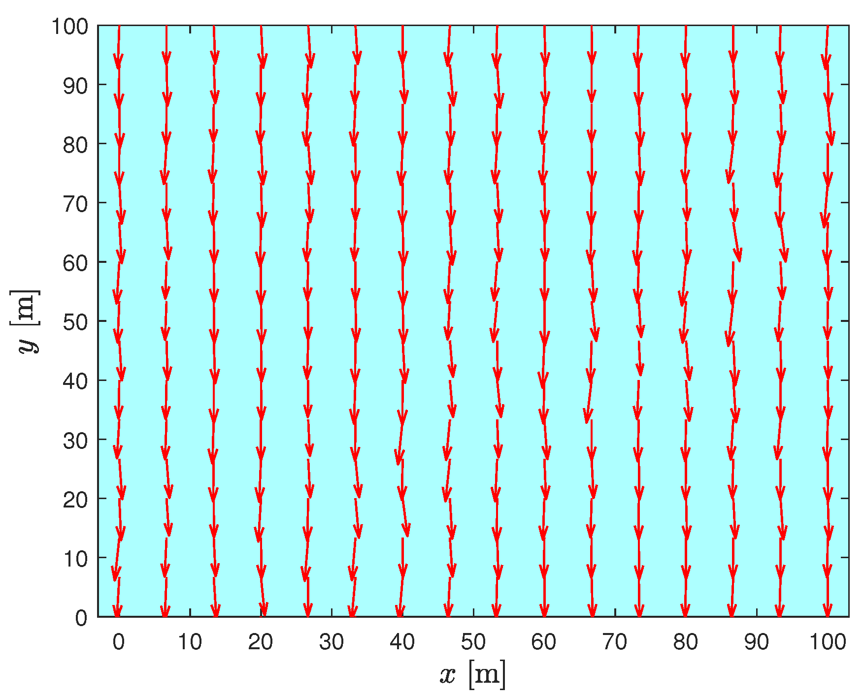
Simulation studies employing the CyberShip II model have been conducted to validate the efficacy of the proposed Prescribed Time Model Predictive Control (PTMPC) strategy. The model parameters are adopted from [37]. And, in particular, m 11 = 25.80 kg , m 22 = 33.80 kg , m 33 = 2.760 kg m 2 . τ ¯ 1 = 200 ( N ) , τ ¯ 2 = 200 ( N ) and τ ¯ 3 = 200 ( N   m ) . The hydrodynamic coefficients d 11 = 12 , d 22 = 17 , d 33 = 0.5 , d n 11 = 2.50 , d n 22 = 4.50 and d n 33 = 0.10 . To accurately emulate real world operational conditions for USVs, realistic environmental disturbances including wind, waves, and currents have been incorporated. A high fidelity physics based wind wave model was implemented by integrating the NORSOK wind spectrum with the JONSWAP wave spectrum, thereby enabling precise simulation of wind and wave induced forces [32]. In the presented simulation, a north wind with a mean speed of 6 m / s is applied. The wave model is configured with a significant wave height of 0.088 m and a peak period of 1.44 s. The forms of the wind spectrum and the wave spectrum are shown in Figure 3 and Figure 4.

6.2. Tracking Performance Validation

The reference trajectory is a sinusoidal shape trajectory and defined as follows:
x d = 0.5 t , y d = 1.8 sin ( 0.5 t ) .
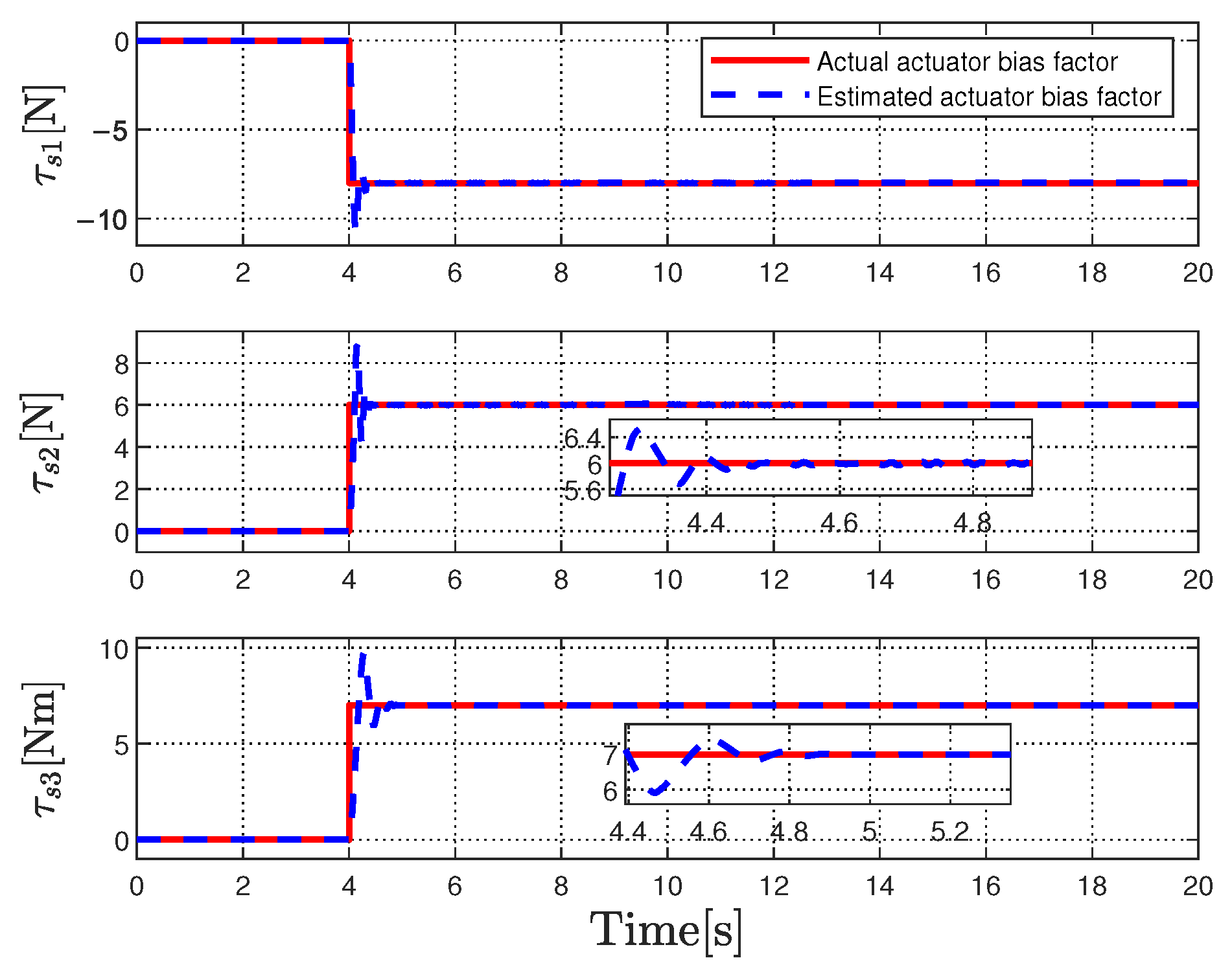
The initial condition of USV is t 0 = 0 , x ( t 0 ) = 0.5 , 0 , π 2 , 0 , 0 , 0 T . For the predefined-time model prediction optimization framework, we select the sampling period δ = 50 ms ; the prediction horizon is T = 12 δ ; the weighting matrices are chosen as Q = diag ( 7 × 10 3 , 7 × 10 3 , 7 × 10 3 , 1 , 1 , 1 ) and R = diag ( 0.003 , 0.003 , 0.003 ) . For the predefined-time fault observer of the auxiliary control system, the parameters are selected as q 1 = 0.6 , T 1 = 0.5 s. The initial condition of the fault and disturbance observer is η ^ ( t 0 ) = 0.5 , 0 , π 2 T , ω ^ ( t 0 ) = 0 , 0 , 0 T , d ^ ω ( t 0 ) = 0 , 0 , 0 T . For the auxiliary controller, we choose T r = 2   s , q 2 = 0.6 , ε = 0.01 . To illustrate the fault-tolerant ability of the developed fault-tolerant control, we simulate the case where the actuators will bias 8 N , 6 N and 7 N m , respectively in the 4 s and the actuators will fail 40 % , 25 % , and 30 % in the 12.5 s, i.e., τ s = 8 N , 6 N , 7 N m T and θ = 0.6 , 0.75 , 0.7 T .
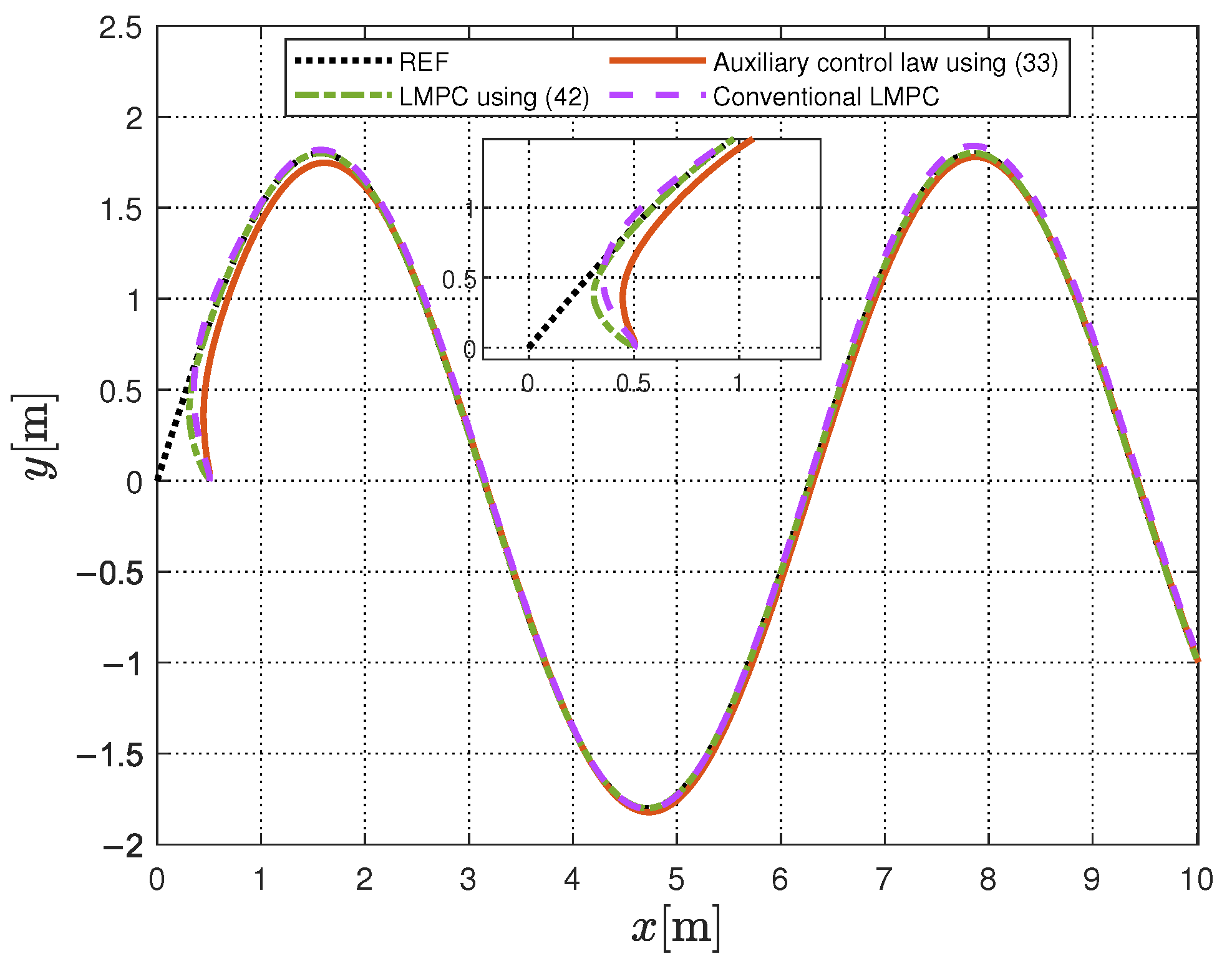
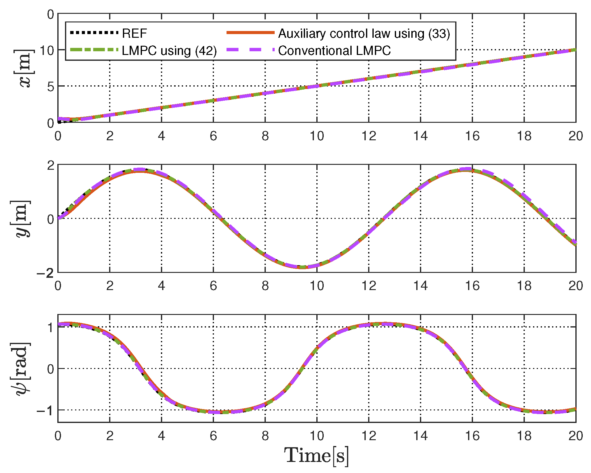
The tracking results for trajectory tracking are presented in Figure 5, Figure 6 and Figure 7. Various methods, including the auxiliary control law derived from Equation (33) and the conventional backstepping-based LMPC algorithm [16], are compared simultaneously. It is important to note that the parameters for both the LMPC-related and auxiliary control laws align with those specified in the PTMPC framework. In Figure 5, the PTMPC optimization strategy is compared with the predefined-time auxiliary control law (33) and the conventional LMPC optimization approach [16] to highlight the advantages of PTMPC in addressing ocean disturbance and actuator fault. It is clear that, in contrast to the conventional LMPC approach, PTMPC ensures a stringent convergence rate, thereby improving optimization performance while maintaining fault tolerance against actuator fault. Figure 6 effectively illustrates the state variation over time during the tracking process, and Figure 7 illustrates the variation in control inputs. Notably, the inputs for each dimension of the auxiliary control law comply with the defined constraints, thereby ensuring the feasibility of the PTMPC optimization problem. Furthermore, the control inputs of FTLMPC exhibit a more rapid response, highlighting the effectiveness of the proposed optimization strategy in mitigating disturbance and actuator fault.
The simulation results of the predefined-time fault observer are shown in Figure 8 and Figure 9. The results show that this method can identify the fault information, includes θ and τ s in a short time.
For disturbances such as wind and wave forces, an LSTM network was trained using historical sensor data and integrated into the USV control system to achieve disturbance prediction capabilities. In the implementation, we selected 1400 input–output samples and set the sliding window length to 5, generating 1394 training sequences. During training, the LSTM network updates its weights using the Adam optimizer with each batch of five consecutive samples, effectively capturing the dynamic relationship between sensor data and marine disturbances. To further evaluate the generalization ability of the designed network, we used an additional 600 samples for predictive performance testing of the trained model. As demonstrated in Figure 10, the LSTM network achieves rapid convergence of prediction errors under irregular sampling intervals and exhibits superior predictive performance during testing.

7. Conclusions

This paper introduces a predefined-time MPC algorithm for USV trajectory tracking, addressing the challenges posed by disturbances and actuator failures. By incorporating contraction constraint, predefined-time sliding-mode auxiliary control system, LSTM-based network, and predefined-time fault observers into the online MPC optimization problem, the proposed method ensures both tracking performance and predefined time stability. Additionally, by integrating fault information observed from the observer and disturbance information predicted by LSTM network into the PTMPC optimization strategy, the algorithm enables more efficient trajectory tracking, thereby optimizing control performance. Simulation results confirm the effectiveness of the proposed approach.
Safety remains a paramount concern in unmanned surface vessel control applications and warrants continued investigation. Future research will emphasize the seamless integration of the proposed model predictive control strategy with physical vessel systems to address practical deployment challenges, thereby ensuring robust performance in real-world maritime environments.

Author Contributions

Conceptualization, Y.Z. and L.-Y.H.; methodology, Y.Z. and H.A.; software, Y.Z.; validation, L.-Y.H.; formal analysis, L.-Y.H.; investigation, L.-Y.H.; resources, L.-Y.H.; data curation, Y.Z. and H.A.; writing—original draft preparation, Y.Z.; writing—review and editing, L.-Y.H.; visualization, Y.Z.; supervision, L.-Y.H.; project administration, L.-Y.H.; funding acquisition, L.-Y.H. All authors have read and agreed to the published version of the manuscript.

Funding

This work was supported in part by the National Natural Science Foundation of China under Grant 52171292 and Grant 51939001; and in part by the Dalian Outstanding Young Talents Project under Grant 2022RJ05.

Data Availability Statement

The original contributions presented in this study are included in the article. Further inquiries can be directed to the corresponding author.

Conflicts of Interest

The authors declare that they have no confict of interest regarding this work.

References

  1. Wei, H.; Shi, Y. MPC-based Motion Planning and Control Enables Smarter and Safer Autonomous Marine Vehicles: Perspectives and a Tutorial Survey. IEEE CAA J. Autom. Sin. 2023, 10, 8–24. [Google Scholar] [CrossRef]
  2. Peng, Z.; Wang, J.; Wang, D.; Han, Q.L. An Overview of Recent Advances in Coordinated Control of Multiple Autonomous Surface Vehicles. IEEE Trans. Ind. Inform. 2021, 17, 732–745. [Google Scholar] [CrossRef]
  3. Hao, L.Y.; Zhang, H.; Guo, G.; Li, H. Quantized Sliding Mode Control of Unmanned Marine Vehicles: Various Thruster Faults Tolerated With a Unified Model. IEEE Trans. Syst. Man Cybern. Syst. 2021, 51, 2012–2026. [Google Scholar] [CrossRef]
  4. Tee, K.; Ge, S. Control of fully actuated ocean surface vessels using a class of feedforward approximators. IEEE Trans. Control Syst. Technol. 2006, 14, 750–756. [Google Scholar] [CrossRef]
  5. Aguiar, A.P.; Hespanha, J.P. Trajectory-Tracking and Path-Following of Underactuated Autonomous Vehicles With Parametric Modeling Uncertainty. IEEE Trans. Autom. Control 2007, 52, 1362–1379. [Google Scholar] [CrossRef]
  6. Hao, L.Y.; Zhang, H.; Li, T.S.; Lin, B.; Chen, C.L.P. Fault Tolerant Control for Dynamic Positioning of Unmanned Marine Vehicles Based on T-S Fuzzy Model with Unknown Membership Functions. IEEE Trans. Veh. Technol. 2021, 70, 146–157. [Google Scholar] [CrossRef]
  7. Yu, K.; Li, Y.; Lv, M.; Tong, S. Adaptive Backstepping Control for Underactuated 6-DoF USV with Uncertain Dynamics. IEEE Trans. Intell. Veh. 2024, 9, 7476–7484. [Google Scholar] [CrossRef]
  8. Song, S.; Park, J.H.; Zhang, B.; Song, X. Event-Triggered Adaptive Practical Fixed-Time Trajectory Tracking Control for Unmanned Surface Vehicle. IEEE Trans. Circuits Syst. II Express Briefs 2021, 68, 436–440. [Google Scholar] [CrossRef]
  9. Lu, R.; Wang, X.; Ding, Y.; Zhang, H.T.; Zhao, F.; Zhu, L.; He, Y. Adaptive Optimal Surrounding Control of Multiple Unmanned Surface Vessels via Actor-Critic Reinforcement Learning. IEEE Trans. Neural Netw. Learn. Syst. 2025, 36, 12173–12186. [Google Scholar] [CrossRef]
  10. Zhang, D.; Ye, Z.; Feng, G.; Li, H. Intelligent Event-Based Fuzzy Dynamic Positioning Control of Nonlinear Unmanned Marine Vehicles Under DoS Attack. IEEE Trans. Cybern. 2022, 52, 13486–13499. [Google Scholar] [CrossRef]
  11. Fossen, T.I. Handbook of Marine Craft Hydrodynamics and Motion Control; Wiley: Hoboken, NJ, USA, 2011. [Google Scholar]
  12. Magni, L.; Raimondo, D.; Scattolini, R. Regional Input-to-State Stability for Nonlinear Model Predictive Control. IEEE Trans. Autom. Control 2006, 51, 1548–1553. [Google Scholar] [CrossRef]
  13. Scokaert, P.; Mayne, D.; Rawlings, J. Suboptimal model predictive control (feasibility implies stability). IEEE Trans. Autom. Control 1999, 44, 648–654. [Google Scholar] [CrossRef]
  14. Hu, B.; Linnemann, A. Toward infinite-horizon optimality in nonlinear model predictive control. IEEE Trans. Autom. Control 2002, 47, 679–682. [Google Scholar]
  15. Shen, C.; Shi, Y.; Buckham, B. Trajectory Tracking Control of an Autonomous Underwater Vehicle Using Lyapunov-Based Model Predictive Control. IEEE Trans. Ind. Electron. 2018, 65, 5796–5805. [Google Scholar] [CrossRef]
  16. Wei, H.; Shen, C.; Shi, Y. Distributed Lyapunov-Based Model Predictive Formation Tracking Control for Autonomous Underwater Vehicles Subject to Disturbances. IEEE Trans. Syst. Man Cybern. Syst. 2021, 51, 5198–5208. [Google Scholar] [CrossRef]
  17. Park, S.; Kim, J.; Kim, J.; Wang, S. Fault Diagnosis of Air Handling Units in an Auditorium Using Real Operational Labeled Data across Different Operation Modes. J. Comput. Civ. Eng. 2025, 39, 04025065. [Google Scholar] [CrossRef]
  18. Wang, S. Automated fault diagnosis detection of air handling units using real operational labelled data and transformer-based methods at 24-hour operation hospital. Build. Environ. 2025, 282, 113257. [Google Scholar] [CrossRef]
  19. Hao, L.Y.; Liu, Y.P.; Wu, Z.J.; Shen, C. Learning-Based Guidance and Control Codesign for Underactuated Autonomous Surface Vehicles: Theory and Experiment. IEEE Trans. Ind. Electron. 2025, 72, 3927–3936. [Google Scholar] [CrossRef]
  20. Yu, J.; Chen, Z.; Zhao, Z.; Deng, H.; Wu, J.; Xu, J. A Cooperative Hunting Method for Multi-USVs Based on Trajectory Prediction by OR-LSTM. IEEE Trans. Veh. Technol. 2024, 73, 18087–18101. [Google Scholar] [CrossRef]
  21. Xu, X.; Zhang, X.; Zhang, Z.; Ma, F.; Guan, C.; Steyskal, F. LOS Guidance for Fuzzy Adaptive Fault-Tolerant Path Following Control of USV With Side-Slip Compensation and Actuator Fault. IEEE Trans. Transp. Electrif. 2025, 11, 6875–6886. [Google Scholar] [CrossRef]
  22. Tong, S.; Zhou, H.; Li, Y. Neural Network Event-Triggered Formation Fault-Tolerant Control for Nonlinear Multiagent Systems With Actuator Faults. IEEE Trans. Syst. Man Cybern. Syst. 2023, 53, 7571–7582. [Google Scholar] [CrossRef]
  23. Chen, L.; Liu, M.; Shi, Y.; Zhang, H.; Zhao, E. Adaptive Fault Estimation for Unmanned Surface Vessels with a Neural Network Observer Approach. IEEE Trans. Circuits Syst. I Regul. Pap. 2021, 68, 416–425. [Google Scholar] [CrossRef]
  24. Zheng, Z.; Sun, L.; Xie, L. Error-Constrained LOS Path Following of a Surface Vessel With Actuator Saturation and Faults. IEEE Trans. Syst. Man Cybern. Syst. 2018, 48, 1794–1805. [Google Scholar] [CrossRef]
  25. Corradini, M.L.; Monteriu, A.; Orlando, G. An Actuator Failure Tolerant Control Scheme for an Underwater Remotely Operated Vehicle. IEEE Trans. Control Syst. Technol. 2011, 19, 1036–1046. [Google Scholar] [CrossRef]
  26. Gu, N.; Wang, D.; Peng, Z.; Liu, L. Observer-Based Finite-Time Control for Distributed Path Maneuvering of Underactuated Unmanned Surface Vehicles With Collision Avoidance and Connectivity Preservation. IEEE Trans. Syst. Man Cybern. Syst. 2021, 51, 5105–5115. [Google Scholar] [CrossRef]
  27. Yang, Y.; Wang, J.; Hua, C.; Li, J. Saturation-Tolerant Adaptive Fixed-Time Control of Underactuated Surface Vessel With Improved Given Performances. IEEE Trans. Intell. Veh. 2024, 1–11. [Google Scholar] [CrossRef]
  28. Hong, Y.; Wang, J.; Cheng, D. Adaptive finite-time control of nonlinear systems with parametric uncertainty. IEEE Trans. Autom. Control 2006, 51, 858–862. [Google Scholar] [CrossRef]
  29. Liu, S.; Wang, H.; Li, T.; Xu, K. Adaptive Neural Fixed-Time Control for Uncertain Nonlinear Systems. IEEE Trans. Circuits Syst. II Express Briefs 2024, 71, 637–641. [Google Scholar] [CrossRef]
  30. Becerra, H.M.; Vázquez, C.R.; Arechavaleta, G.; Delfin, J. Predefined-Time Convergence Control for High-Order Integrator Systems Using Time Base Generators. IEEE Trans. Control Syst. Technol. 2018, 26, 1866–1873. [Google Scholar] [CrossRef]
  31. Pan, J.; Han, T.; Xiao, B.; Yan, H. Predefined-Time Bipartite Time-Varying Formation Tracking Control of Networked Autonomous Surface Vehicles via Hierarchical Control Approach. IEEE Trans. Veh. Technol. 2024, 73, 9536–9545. [Google Scholar] [CrossRef]
  32. Fossen, T.I. Marine Control Systems: Guidance, Navigation, and Control of Ships, Rigs, and Underwater Vehicles; Marine Cybernetics: Trondheim, Norway, 2002. [Google Scholar]
  33. Liu, H.; Hao, L.Y.; Che, W.W. Bi-LSTM-Based Resilient Data-Driven Integral Sliding Mode Control for UMVs Under Hybrid Attacks. IEEE Trans. Intell. Transp. Syst. 2025, 26, 6702–6714. [Google Scholar] [CrossRef]
  34. Gao, H.; Huang, Z.; Diao, R.; Zhang, J.; Hou, B.; Wu, C.; Sun, F.; Lan, T. A Machine Learning-Based SVG Parameter Identification Framework Using Hardware-in-the-Loop Testbed. IEEE Trans. Power Syst. 2024, 39, 6849–6860. [Google Scholar] [CrossRef]
  35. Zhou, R.; Hu, C.; Ou, T.; Wang, Z.; Zhu, Y. Intelligent GRU-RIC Position-Loop Feedforward Compensation Control Method With Application to an Ultraprecision Motion Stage. IEEE Trans. Ind. Inform. 2024, 20, 5609–5621. [Google Scholar] [CrossRef]
  36. Jia, C.; Liu, X.; Li, X.; Xu, J. A New Adaptive Predefined Time Sliding Mode Control for Nonlinear Systems. IEEE Trans. Circuits Syst. II Express Briefs 2024, 71, 2094–2098. [Google Scholar] [CrossRef]
  37. Skjetne, R.; Fossen, T.I.; Kokotović, P.V. Adaptive maneuvering, with experiments, for a model ship in a marine control laboratory. Automatica 2005, 41, 289–298. [Google Scholar] [CrossRef]
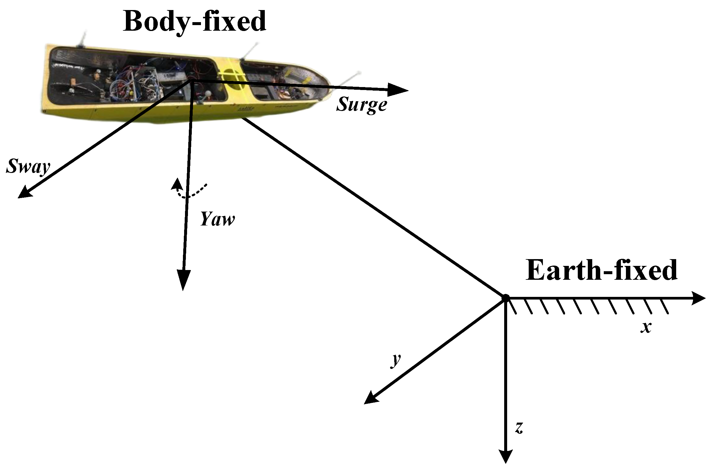
Figure 1. A typical USV model with three degrees of freedom (The yaw velocity is defined by the rate of change of the dashed path).
Jmse 13 01914 g001
Figure 2. LSTM-based predefined-time MPC strategy structure diagram.
Jmse 13 01914 g002
Figure 3. Two-dimensional view of sea winds (The orientation of the arrow indicates the wind velocity vector).
Jmse 13 01914 g003
Figure 4. Three-dimensional view of the sea waves.
Jmse 13 01914 g004
Figure 5. The USV trajectories with different algorithms (REF indicates the reference trajectory, and the conventional LMPC strategy is designed in [16]).
Jmse 13 01914 g005
Figure 6. State trajectories of USVs with different algorithms (the conventional LMPC strategy is designed in [16]).
Jmse 13 01914 g006
Figure 7. Control signals of USVs with different algorithms (the solid black lines illustrate the physical constraints on the marine thrusts, and the conventional LMPC strategy is designed in [16]).
Jmse 13 01914 g007
Figure 8. Actuator bias factor estimations for τ ^ s .
Jmse 13 01914 g008
Figure 9. Actuator failure factor estimations for θ ^ .
Jmse 13 01914 g009
Figure 10. Disturbance estimations of LSTM-based network for τ ω .
Jmse 13 01914 g010
Disclaimer/Publisher’s Note: The statements, opinions and data contained in all publications are solely those of the individual author(s) and contributor(s) and not of MDPI and/or the editor(s). MDPI and/or the editor(s) disclaim responsibility for any injury to people or property resulting from any ideas, methods, instructions or products referred to in the content.