Computational Fluid Dynamics Prediction of the Sea-Keeping Behavior of High-Speed Unmanned Surface Vehicles Under the Coastal Intersecting Waves

Abstract

To better study the sea-keeping response behavior of unmanned surface vehicles (USVs) in coastal intersecting waves, a prediction is conducted using the CFD method in this paper, in which a USV with the shape of a small-scale catamaran and designed target for high-speed navigating is considered. The CFD method is proved to be good enough at ship response prediction and can be utilized in abundant forms of towing experiment simulations, including planar motion mechanism experiments. The regular and irregular wave generation of numerical CFD can also virtualize the actual wave tank work, making it equally scientific but more efficient than the real test. This research regards the changing trend of encounter characteristics of USVs meeting two trains of waves with different inclination angles and wavelengths by monitoring wave profiles, pitch, heave, acceleration, slamming force, and pressure on specific locations of the USV hull. This paper first introduces the modeling method of intersecting waves in a virtual tank and verifies the wave profiles by comparing them with a theoretical solution. Further, the paper focuses on the sea-keeping motion of USVs and analyzes the complicated influences of encounter parameters. Eventually, this paper analyzes the changing pattern of the motion in encounter frequency and investigates the severity during the sea-keeping period through acceleration analysis.

1. Introduction

Unmanned surface vehicles (USVs) are increasingly being deployed to meet the growing demands of maritime operations, such as maritime defense, island reefs, and nearshore patrols [1]. However, nearshore oceans are filled with unexpected and complex waves [2]. For an autonomous sailing USV, precisely perceiving the encounter wave characteristics to accordingly take efficient and safe navigational routes is important, and this has been ignored in USV research. The traditional method of using hydrodynamic experiments with fixed or towed models is usually only able to generate a single directional wave train and is also costly. Nowadays, researchers of USVs pay great attention to their navigation algorithms in calm water, yielding insufficient experiments on sea-keeping response in possible extreme environments. In fact, different wave profiles and navigating strategies will induce different sea-keeping reactions, and the steep accelerations, green waters, and damping forces applied on the hull will damage the structures. Navigating at a relatively high speed and in a proper direction may shorten the process in the wave region, which is desirable, but the resultant transverse and vertical wave loading have unknown influences. Meanwhile, ship response in different situations needs to be studied when navigating while following waves whose direction of travel is the same as a USV with a planning type hull. USVs are usually designed for high-speed operations, which may introduce more severe conditions in wave encounters [3]. Thomson J [4] compared the rising draft tendencies of the V15 hull at different speeds of 3.31, 4.26, and 5.21, and initial trim angles of 4, 3, and 2.2, respectively, in still water. Studies generally reveal the dynamic response of the hull near steady-state conditions in high-speed scenarios. Sun H [5] focused on the motion response of an SSB catamaran under regular waves with frequency velocities between 0.11 and 0.4, considering wave/ship length ratios (λ/L) ranging from 0.5 to 1.75, and the results showed that encountering specific wave periods led to resonant responses. The response characteristics of planning craft under unidirectional regular waves have been extensively observed to be related to speed resonance peaks. Diez et al. [6,7] investigated the motion response characteristics of a 3 m scale Deft catamaran model under irregular waves with a significant wave height of 0.0975 m and regular waves with a significant wave height of 0.061 m. The results indicate that the heave motion amplitude is close to 100 mm in regular waves, with a pitch angle range within 6°. In practice, USVs are expected to be considerably utilized in canals and coastal areas, where complicated ship waves of multiple ships reflect and intersect, complicating the hydrology and potentially leading to unexpected responses, influencing the structure safety and the navigating efficiency. Especially for high-speed, small-scale USVs, their behavior is still worthy of further investigation.

The phenomenon of intersecting wave superposition [8] is widely observed in coastal areas. The reflecting waves intersect with the original waves, including swells and ship waves, making the intersecting waves more common in the coastal region, and highly overlap with the mission areas of civil and military USVs. The intersecting phenomenon will strengthen the wave severity and the slamming loading on the ship hull. The complicated hydrodynamic effect in the square field influences the navigating speed and the sea-keeping amplitude of USVs. Great impact also damages the structure and the equipment. In the estuary of the Qiantang River in East China, rectangular waves have been listed as one of the typical intersecting wave forms, as shown in Figure 1, reported by Xinhua News Agency. This is a result of different ocean currents coming from two different weather systems joining each other at coastal areas, most commonly at the edge of the continent. However, its influence on a high-speed USV is unknown. Intersecting waves and spilling breakers are special waves observed regularly in the Qiantang River tidal bore. An annual tidal surfing competition has been held there for over ten years, during which smaller escort ships need to patrol the corresponding sea areas. It is noteworthy that intersecting waves widely take place all around the world, typically in the coastal areas of the Pacific Ocean and the Atlantic Ocean, such as at the Isle of Rhe in France and Anna Maria Island, Florida, USA. Cavaleri [9] investigated extreme-wave-related accidents at sea, resulting in fatalities in two shipwrecking incidents. They found that intersecting wave systems with similar energy levels and inclination angles of 40–60 degrees could be responsible for these occurrences. Reference [10] demonstrated that the world-famous “New Year Wave” incident, which hit the Draupner oil platform in the Norwegian North Sea, could be the result of intersecting wave spectra formed by wave trains with an inclination. The dynamic impact of these complex waves on ships has uncertain characteristics that deserve further attention.

In this domain, Jiao et al. [11] proposed a numerical experiment to simulate wave-induced motions of the S175 ship in orthogonal encounters with intersecting waves. Huang et al. [12] further designed a series of studies discussing the different characteristics of intersecting waves and unidirectional regular waves on the S175 container ship model at various heading angles, setting the ship’s speed to Fr 0.25. Chen et al. [13] mainly investigated the performance of a trimaran ship with a length of 143 m in transverse waves with a λ/L ratio between 0.6 and 1.2, with the highest simulation speed within the range of Fr 0.4. The simulating conditions above are far from extreme and high-speed for a large scale ship, and it is notable that in previous studies of intersecting waves on ships, only orthogonal superposition cases have been mentioned and ships are simulated in only a straightforward trajectory. However, according to values from [14,15], the energy of intersecting waves largely depends on their inclination angle, and there are different amplitudes at different concentration locations, which influence the strategy. Thus, the sea-keeping responses of USVs when encountering wave spectra of different inclination angles deserve further analysis, so as to perceive the wave form and plan a safer route. Additionally, the influence of these waves on small-scale USVs driven at high speeds has also been rarely emphasized by researchers. The uncertain nonlinear effects could pose challenges to the maneuverability of fast boats. Efficiently passing through wave fields at high speeds and dealing with the accompanying intense wave actions require effective research to balance the safety and efficiency.

The methods to study the wave–ship interaction include towing tanks and numerical methods. Towing tanks have been widely used for regular wave research; nevertheless, the simulation difficulty and experimental costs are high for towing ships under special forms of nonunidirectional waves. In numerical methods, the computational fluid dynamics (CFD) method can more effectively account for fluid viscosity and boundary layer effects, making it theoretically more accurate than potential flow methods [16,17]. This is particularly relevant in the case of planning catamarans, where the viscous effects considered by CFD theory can better capture the variations in hydrodynamic lift between the two hulls and the impact forces of the waves [18,19].

Before this proposal, CFD methods have been widely used to explore marine structures. Khang Minh Phan [20] studied the extreme responses of standard KCS ships in single-directional regular waves. Long-crested waves [21] generated by superimposing different wavelengths and amplitudes have also been extensively studied to reveal the interaction patterns between waves and marine structures. Yu [22] established a maneuvering model for ships under long-crested irregular waves without random direction, which was applied for steering simulations of the S175 model. Wang et al. [23] aimed to achieve a more realistic coastal wave description and successfully implemented a multidirectional irregular wave in REEF3D, a CFD tool developed by the Norwegian University of Science and Technology. Li et al. [24] applied multidirectional waves to vertically floating cylinders to reveal the interaction between waves and structures. Liu et al. [25] considered fixed horizontal semi-submerged cylinders under irregular and regular waves. Zhang et al. [26] considered the effects of short-crested waves on a 120 m Lpp trimaran from aspects such as sea-state effects, velocity effects, and wind effects to evaluate the increased resistance and speed loss, employing CFD tools to validate irregular spectra. Kim [27] investigated the maneuvering of the KCS model in a series of rough long-crested irregular waves using a CFD RANS model to better represent the motion in real sea conditions.

In the majority of CFD simulation studies mentioned above and in [26,28,29,30,31], ships are set as stationary in the direction of incoming waves, and a single wave speed is set to represent the relative motion, with the current speed as a major objective parameter. Nevertheless, the stationary description cannot account for the situations where the ship is navigating in varying directions. An effective method to describe the relative motion of ship and wave speed is the planar motion mechanism (PMM). The numerical PMM tests are generally adopted for ship maneuverability studies in calm water [32,33,34], and are also used in head-wave situations [35,36,37], but are seldom employed to look into ships’ responses to different sailing routes in complicated intersecting waves. The interspersed crests and troughs in the superimposed wave field, indeed, suggest that exploring more flexible navigation trajectories is a worthwhile area of investigation.

Hence, a series of CFD experiments and relevant theoretical derivations is conducted in this paper. A numerical towing tank is established, and intersecting waves in different encounter situations, inducing different parameters, are considered in Section 3. In addition, a more precise theoretic solution is innovatively adopted to verify the intersecting wave elevation. In Section 4, the sea-keeping response motion of USV influenced by different parameters is examined by comparing the encountered wave elevations and the vertical response motion form, in which crucial influences of different navigating strategies are revealed. In Section 5, RAO analysis is adopted to compare the severity of vertical motion to investigate the alteration trends in different encountered situations. Accelerations associated with pressure on different regions of the hull structure are examined. The detailed characteristics of acceleration are also studied, and show consistency with the encountered wave speed. Furthermore, by understanding the relationship between the severity of acceleration and wave phase during different encounter periods, several efficient route schemes with gentler encounter responses are proposed and verified through pure sway tests to reduce the severity of acceleration response amplitudes.

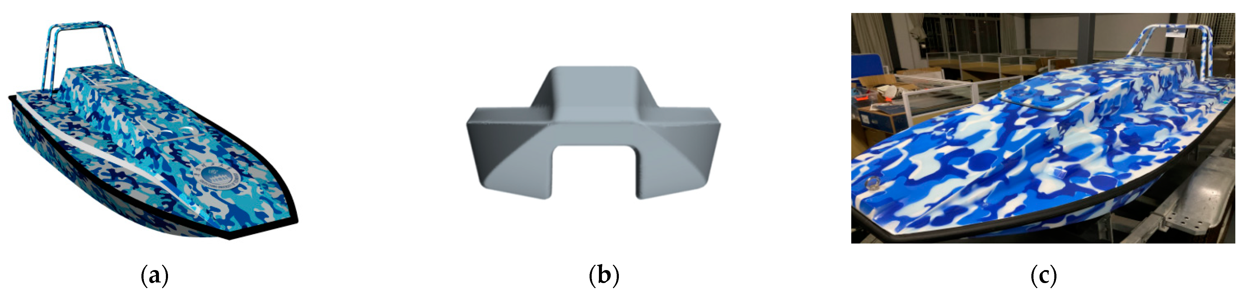
2. Geometry Modeling of the Fast Ship

To investigate the motion response and load response of a small fast boat in intersecting waves, an SCUTME-22 USV, as shown in Figure 2c, was selected as the research subject. This boat is constructed with carbon fiber and fiberglass (fiber-reinforced plastics) materials and has a small catamaran hull design, as shown in Figure 2a. For efficiency of calculation, the necessary simplicity for the trestle structure in the rear part of the model that is above the water is performed, as shown in Figure 2b. The main dimensional parameters of the boat model are given in

Table 1. Catamaran main dimensions.

Characteristic Item	Value
Scale (k)	1:1
Length between perpendiculars (Lpp)/m	2.7283
Beam overall (B)/m	1.167
Beam between center of demihull (Bd)/m	0.8
Demihull beam (Db)/m	0.367
Depth (D)/m	0.729
Draft (d)/m	0.254
Displacement (Δ)/kg	208.5
Vertical center of gravity from BL (VCG)/m	0.433
Longitude center of gravity form AP (LCG)/m	1.0785
Demihulls separation (Dp)/m	0.415
Demihull height (Dh)/m	0.249

. The model of the boat has a scale ratio of 1:1, and the immersion part of the hull is described as two demihulls. The geometry of the hull is quantified using the single demihull height, the beam between their centers, and the separation between them. The location of the CG is defined using the relative two perpendiculars according to the ITTC symbols list [38].

3. Implement of the Intersecting Waves

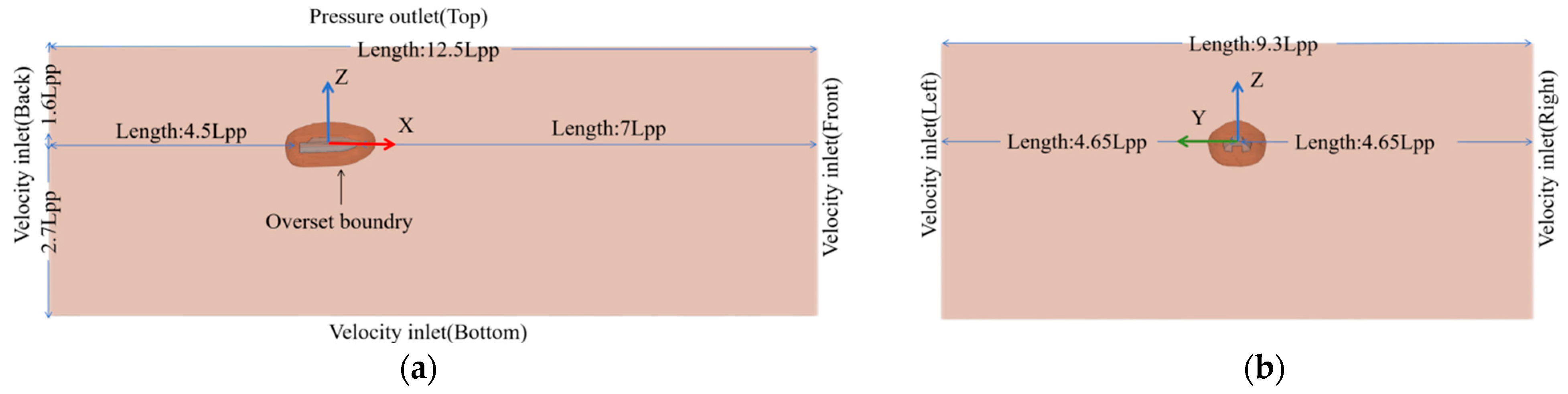
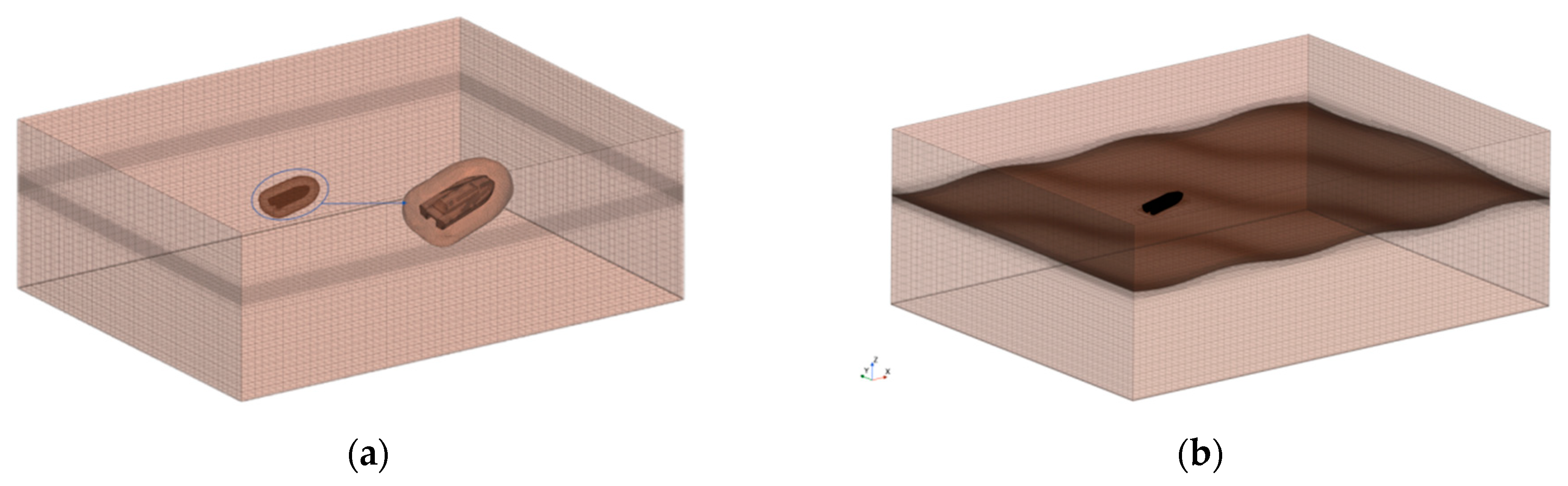
3.1. Physical Modeling of the Numerical Tank

This article uses the commercial software Star-CCM+ to calculate the sea-keeping behavior and wave load characteristics of a dual-body USV in various intersecting waves. The RANS [39] method and the two-layer realized-k-ε [40,41] numerical method have been proven valid in CFD simulations, as demonstrated in [42,43], both of which have broad influences in the field of ship and ocean engineering. According to [44], the continuity and momentum equations for unsteady incompressible flows processed using the Reynolds time-averaging method are shown in tensor notation in Equations (1) and (2), where $\rho$ means density and $\overline{u_i},x_i$ means average velocity and the Cartesian coordinates component. In order to solve the transport equations, the Reynolds stress component $\overline{{u^{\prime }}_i{u^{\prime }}_j}$ is further expressed by Boussinesq assumption of eddy viscosity in Equation (3), in which $k$ is turbulence kinetic energy, ${\nu }_t$ is turbulence viscosity, and ${\delta }_{ij}$ is Kronecker delta operator. Meanwhile, the Eulerian multiphase flow model is used to describe the two-phase flow of water and air, and the VOF (volume of fluid) model is employed to capture the stratification of the free surface between water and air. In this study, the VOF model uses a second-order convection scheme to calculate the volume fraction of water and air in each discrete volume unit. A value of 0.5 represents a 50% occupancy of both dense fluid (liquid water) and light fluid (air), indicating the position of the ship’s waterline.

$${\displaystyle \frac{\partial (\rho \overline{u_i})}{\partial x_i}}=0$$

(1)

$${\displaystyle \frac{\partial {\overline{u}}_i}{\partial t}}+{\displaystyle \frac{\partial }{\partial x_j}}\left({\overline{u}}_i{\overline{u}}_j\right)-{\displaystyle \frac{\partial }{\partial x_j}}\left[\nu ({\displaystyle \frac{\partial {\overline{u}}_i}{\partial x_j}}+{\displaystyle \frac{\partial {\overline{u}}_j}{\partial x_i}})-\overline{{u^{\prime }}_i{u^{\prime }}_j}\right]=-{\displaystyle \frac{1}{\rho }}{\displaystyle \frac{\partial \overline{p}}{\partial x_i}}$$

(2)

$$-\overline{{u^{\prime }}_i{u^{\prime }}_j}={\nu }_t\left({\displaystyle \frac{\partial \overline{u_i}}{\partial x_j}}+{\displaystyle \frac{\partial \overline{u_j}}{\partial x_i}}-{\displaystyle \frac{2}{3}}{\displaystyle \frac{\partial \overline{u_k}}{\partial x_k}}{\delta }_{ij}\right)-{\displaystyle \frac{2}{3}}k{\delta }_{ij}$$

(3)

The numerical discretization strategy for the USV employs the finite volume method (FVM) in a formulation that applies an implicit unsteady iteration scheme with second-order spatial discretization. In this way, the governing equation of the viscous model can be solved on the finite cells, where the decoupling of the velocity and pressure term can be calculated in parallel. In cases of steady flow, the time step size can be determined based on the Courant criterion, also known as Courant Friedrichs Lewy (CFL), which quantitatively constrains the minimum distance that a fluid can travel through the grid within a unit time step. However, for implicit unsteady flow, the time accuracy is related to the flow period. The ITTC recommends including at least 100 time steps within each period. In this paper, the basic time step and adaptive time step are used together. When local CFL exceeds the limit, the adaptive time step will be adopted and running at an interval of 0.0025 s, roughly 1‰ of the wave period, and the overset boundary mesh is also set to autonomously update every time step, ensuring that the donors and acceptors match properly.

To compute the wave-induced forces and moments on the ship hull and monitor the ship’s sea-keeping behavior, the dynamic fluid–body interaction (DFBI) model is employed to solve the rigid body motion control equations under specific freedom constraint conditions for the USV. According to [45,46,47], the general governing equations under multidimensional towing constraints can be expressed as follows. The towed ship is mounted on a partially constrained coordinate system. $p$ is utilized to represent the generalized independent coordinate vector in Equation (4), where nc is the amount of affine freedom degree. The linear speed and angular speed of the towed object can be described with the differentiation of position vector $r\left(p,t\right)$ and the orientation matrix $T\left(p,t\right)$ in reference coordinates with respect to time, as per Equations (5) and (6), meaning that the overall motion status rests with the coordinates status and the relative motion. Equation (7) shows the Newton dynamic governing equation, in which $F_{\mathrm{g}}$ represents generalized force and moment vectors, including the necessary force that maintains the towing motion of the reference system and the inside or outside environmental loading. In order to represent the relative motion of the ship and the wave more clearly and to explore the result of a changing relative wave speed, three degrees of freedom motion of the USV are defined with PMM, and the others are allowed to drift according to waves without additional constrains. The x-axis is defined as the direction of navigation and the speed, ranging from Fr 0.39 to 1.55. The PMM control law is defined in Equations (8) and (9) shown below, determining the surging, swaying, and yaw motions. The three controlling freedoms of longitude, transverse, and heading direction are defined, respectively, by towing speed, lateral swaying amplitude, swaying frequency, and bow angle. The follow-up motion of the ship in the navigation direction is assigned to the computational domain, maintaining the same speed as the surrounding water and keeping the ship’s position relatively fixed to capture the updated wave field throughout the ship’s voyage.

$$p={\left(p_1,p_1,\dots ,p_{6-nc}\right)}^T$$

(4)

$$v={\displaystyle \frac{\partial r\left(p,t\right)}{\partial p}}\dot{p}+{\displaystyle \frac{\partial r\left(p,t\right)}{\partial t}}$$

(5)

$$\omega ={\displaystyle \frac{\partial T\left(p,t\right)}{\partial p}}\dot{p}+{\displaystyle \frac{\partial T\left(p,t\right)}{\partial t}}$$

(6)

$${\left(\mathrm{m}\dot{v},M\dot{\omega }\right)}^T=F_{\mathrm{g},\mathrm{p}}+F_{\mathrm{g},\mathrm{f}}$$

(7)

$$r={\left(V_{0}t,y_0\sin \left(2\pi ft\right),z\right)}^T$$

(8)

$$T=\left(\begin{array}{ccc}\cos \theta \cos \psi & \sin \varphi \sin \theta \cos \psi -\cos \varphi \sin \psi & \cos \varphi \sin \theta \cos \psi +\sin \varphi \sin \psi \\ \cos \theta \sin \psi & \sin \varphi \sin \theta \sin \psi +\cos \varphi \cos \psi & \cos \varphi \sin \theta \sin \psi -\sin \varphi \cos \psi \\ -\sin \theta & \sin \varphi \cos \theta & \cos \varphi \cos \theta \end{array}\right),\mathrm{s}.\mathrm{t}.\psi =\cos (2\pi ft)$$

(9)

To capture the sea-keeping behavior of the ship, the computational domain is divided into two nested regions: the background region representing the water domain, and the overset region fixed on ship coordinates. The hull is bound to the overset region in order to solve flow around the ship surface, and full overset techniques can be found in [48]. The overset region enables the ship to move together with the surrounding mesh grids [49] and exchange flow information with the background water body through a linear interpolation. The overset region outer boundary is established by offsetting the ship’s hull from its geometric center by 0.8 m, with the ship’s surface set as a nonslip wall where the normal and tangential velocities are zero and the outer surface of deviation is set as an overlapping surface. To reduce boundary reflection effects, ITTC [50,51,52,53,54,55] recommends that the background region of the towing tank be established as at least 4 Lpp in the longitude x-direction, 3 Lpp in the lateral y-direction, and 3 Lpp in the vertical z-direction for the computation domain. In order to allow the waves with long wavelengths to fully develop in the region, the domain of the computational region is set to extend 7 Lpp ahead of the ship, 4.5 Lpp behind the ship, and 4.65 Lpp on each side, with 1.6 Lpp above the water surface and a water depth of 2.7 Lpp, illustrated as Figure 3. The inlet spacing in front of the ship is appropriately enlarged so that waves can pass through half or a complete period in front of the ship. As for the boundaries, the front, back, left, and right sides of the towing tank are all defined as velocity inlets to simulate waves coming from different directions, and wave absorption zones are also set. To simulate the condition of infinite water depth, the bottom surface is set as a velocity inlet, and the top surface is set as a pressure outlet, with the outlet pressure defined as standard atmospheric pressure. The Eulerian multiphase flow enters the computational domain through the velocity inlet, exchanges flow data via the overlapping surfaces of the two regions, and ultimately affects the ship’s hull surface. To reduce the influence of incident waves, all velocity inlets are set with wave force boundary conditions, and the wave force length is set to 6 Lpp.

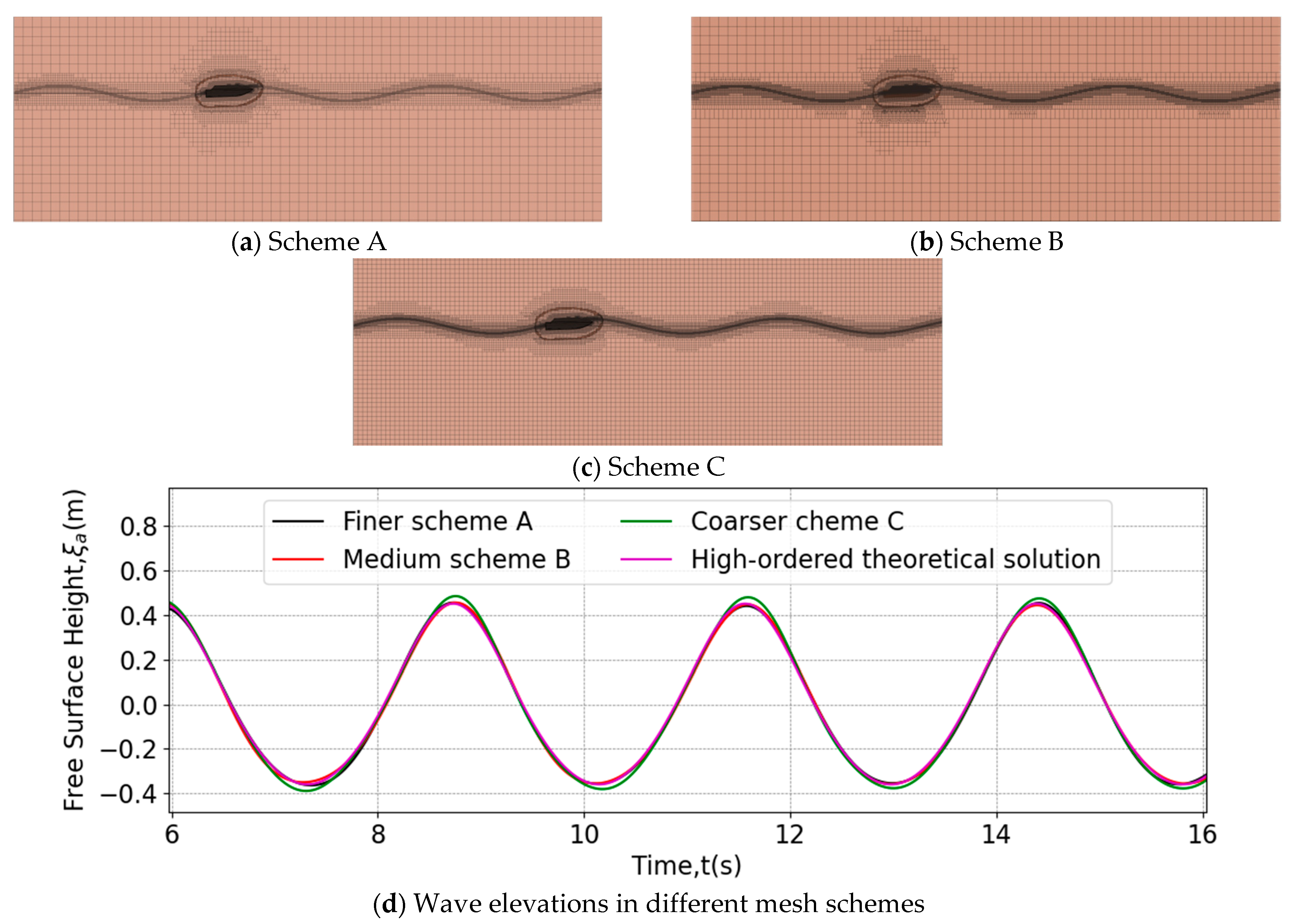
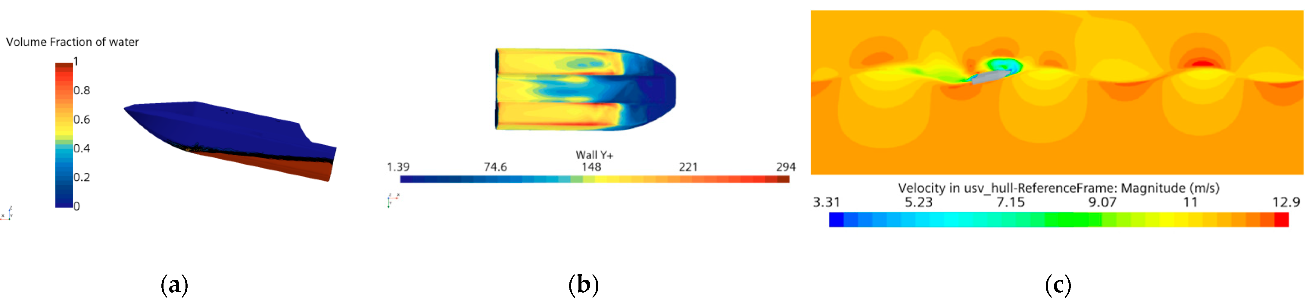
3.2. Meshing and Grid Verification of Numerical Region

The smallest grid size of the ship hull surface is set to 0.024 m, and the layer thickness of the prism is 0.00075 m. Twelve layers of prisms are set to ensure that the wall y+ is between 30 and 300. To ensure that there are 80 grids within the shortest wavelength of the sub-wave and 12 grids within the minimum wave height range, an adaptive grid refinement method is adopted to perform a second adaptive refinement on the free surface. The refinement layer is updated once per time step. To optimize the utilization of computational resources, the grid size in the nonrefined water body region is set to 0.5 m. The overset region is meshed with around 1.5 million unstructured trimmed hexahedral meshes. For the interpolating between overset region and background region, an adaptive updating method is utilized to capture the boundary layer. The meshes split from the core grids and remain as 5–6 layers for every resolution degree and finally form the donor grid around the overset region, forming the overlapping area where the cell is of similar size to the boundary cell of overset grid. The number of grids in the overlapping area is 1.7 million. The free surface is also set as adaptive and the refined level is set to three times, which means that the grid size is continuously averaged and divided by eight based on the custom anisotropic dimensions in the water-surface refined zone, to achieve the grid accuracy required for simulating the wave near the free surface.

According to the ITTC guidelines 2021 and 2024 recommendations, proper verification parameters schemes are expected to be refined at an constant ratio ($r_k=\Delta x_{k_{m+1}}/\Delta x_{k_m}$) of increment, and r_k values varying in $\sqrt{2}\le r_k\le 2$ are acceptable. In a three-scheme convergence analysis, the corresponding convergence evaluating standard of the target parameters is defined as an convergence ratio $R_k={\epsilon }_{kBC}/{\epsilon }_{kAB}$, with respect to the deviation ${\epsilon }_{kij}=S_{ki}-S_{kj}$, as mentioned in [56].

Under premise of |R_k| ≤ 1, a monotonic convergence is achieved when R_k > 0, but it turns out to be oscillation convergence when R_k < 0. The available calculation method is $U_k=F_S\left({\epsilon }_k/(r_k^{p_k}-1)\right)$ for uncertainty under monotonic convergence and $U_k=0.5|\Delta S_k|$ for oscillation situation according to the GCI analysis, as mentioned in [57,58], where $\Delta S_k$ is the oscillation range. The safety factor Fs can be selected as 1.25 and the order of observed accuracy can be selected as 1.97 under the second-order discretion degree; a similar setting was used in [59,60].

Based on the size of the anisotropic dimensions in the water surface refinement area, three different grid densities are utilized with distinct refinement strategies, with an initial grid count of 18 million, 25 million, and 36 million for schemes A, B, and C, respectively, as shown in Figure 4. In scheme A, the adaptive level is limited to two, which results in a coarser mesh near the free surface. In scheme B, the adaptive level is increased to three. In scheme C, the center grid is further refined and the mesh near surface is also refined based on a finer core grid. A time step of $\Delta t=0.01\mathrm{s}$, equal to 4/1000 of the wave period, is selected for adopting mesh verification work along with the initial wave parameters of λ/L = 3.3, inclination angle = 60 deg, and Fr = 1.593. The results are shown in

Table 2. Grid verification results.

	Wave Amplitude/m	Pitching Amplitude/°	Maximum Slamming Force in Z-Direction/N
Scheme A	0.4363	16.273	2117.63
Scheme B	0.4065	15.278	1967.22
Scheme C	0.4012	15.052	1919.41
${\epsilon }_{kBC}$ (%)	1.304	1.479	2.430
${\epsilon }_{kAB}$ (%)	7.33	6.513	7.646
$R_k$ (%)	17.785	22.714	31.786
$U_k^{BC}$ (%)	1.790	1.759	2.889

.

By comparing the initialization of the wave profile with the other two grid schemes, the grid scheme with moderate density demonstrates sufficient ability to capture the free surface edges, and it is ultimately selected for the subsequent case experiments. Wave probe data are shown in Figure 4d, where some slight diverges can be seen in the coarser scheme, and the other schemes are quite smooth and match well enough with the theoretical solution. As shown in Table 2, where wave amplitudes are processed as the half-range between the trough and crest heights, there is a notable decline from ${\epsilon }_{kAB}$ to ${\epsilon }_{kBC}$, resulting in a relatively small convergence ratio. The wave amplitude exhibits monotonic convergency. A similar convergency trend is observed in pitching monitoring and the convergence ratio is around 22.714%. Additionally, there is a much smaller change in the maximum slamming force measurement between B and C, compared to between A and B, indicating that the measurements tend to converge at scheme B, and the uncertainties for these two targets are 1.790%, 1.759%, and 2.889%, all within 10%, suggesting that the grid scheme is adequate. Therefore, medium scheme B is adopted for its calculation efficiency and favorable mesh resolution.

3.3. Time Step Verification

As recommended by the ITTC for time step selection in ship–wave simulations, the time step should be less than 1/100 of the wave period. Thus, three time step schemes, i.e., 6/1000 ($\Delta t=0.015\mathrm{s}$), 4/1000 ($\Delta t=0.01\mathrm{s}$), and 2.6/1000 ($\Delta t=0.0065\mathrm{s}$), of the wave period are adopted for the verification, representing the scheme A, B, C, respectively. The value of rk is 1.5 for these selections. For the implicit methods of unsteady simulation, the CFL criterion is not strictly limited within 1, as it is in explicit problems (referenced in [52]), but is preferred to be within 5 for this simulation. An adaptive time step strategy of 0.0025 s is employed in case the CFL number exceeds 5 in localized regions, with a constant time step otherwise. Initial conditions of λ/L = 3.3, Fr = 1.593, and intersecting waves with inclination angle of 60 deg are selected as the verification case, in which a medium grid scheme B is utilized. The verification results are presented in

Table 3. Time step verification results.

	Wave Amplitude/m	Pitching Amplitude/°	Maximum Slamming Force in Z-Direction/N
Scheme A	0.4128	15.625	2042.91
Scheme B	0.4065	15.278	1967.22
Scheme C	0.4022	15.049	1932.84
${\epsilon }_{kBC}$ (%)	1.075	1.499	1.747
${\epsilon }_{kAB}$ (%)	1.575	2.271	3.848
$R_k$ (%)	68.254	65.994	45.422
$U_k^{BC}$ (%)	1.099	1.532	1.786

.

As shown in Table 3, it can be observed that scheme B–C performs similarly in each result and the divergence in wave amplitude and pitching amplitude is not very notable, which means that scheme C does not show a substantial improvement against Scheme B with time refinement. It can be confidently concluded that, with rather low uncertainty of 1.099% in wave elevation, 1.532% in motion monitoring, and 1.786% in force calculation, the 4/1000 period time step scheme with the adaptive strategy is enough for discretion of the speed and pressure calculation in the field.

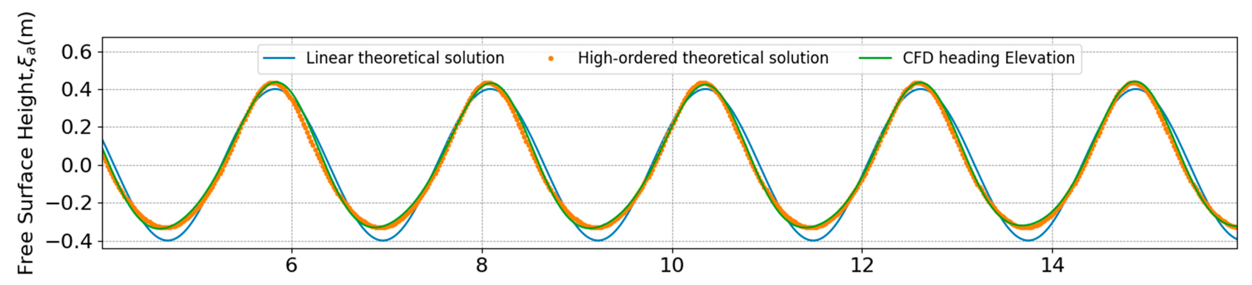
3.4. Validation of Numerical Model

Consider that intersecting waves from two directions together with towing carriage will bring inevitable secondary reflecting in a towing tank of restricted water, disturbing the original intersecting wave field. Thus, an indirect validation method is adopted, using decay motion of USV in calm water, as referenced in [61,62,63,64,65,66], and a CFD model with overset grids is set with an initial trim angle and allowed to undergo free oscillation motion. This approach enables monitoring of the CFD results for natural vertical stability periods, which can then be compared with the experimental properties of the actual hull, previously validated during hull design and fabrication.

In the natural decay tests, three groups of initial conditions are considered, respectively, for the pitching and heaving tests in calm water. The boundary conditions in the CFD setting remain the same as those in Section 3.1. In the heave period test, the hull is released at an initial height either above or beneath the natural draft surface and is allowed to performed free oscillations in vertical plane. In the pitching period test, the initial trim angle is limited to within 15° to avoid the coupling effect of heave and pitching. The ship model test environment is shown in Figure 5. The natural decay motion goes through a gradual attenuation process and the period is calculated as the average value of the time interval between two consecutive crests and troughs during the entire processes. As referenced in [67,68,69], the theoretical period of pitching and heave motion can be expressed as Equation (10), where $I_y,\Delta I_y$ is the moment of inertia and added inertia in the Y-axis, $D_m,\Delta I_z$ is displacement and added mass of ship, $\overline{G{M}_L}$ is longitude metacenter height, and $A_w$ is the area of water plane. The calculation of added mass of water and the wet surface will also inevitably introduce error, and for convenience, empirical formulas are used to generally indicate the rough range of period and are listed as Equation (11), where $C_{\varphi }$ is the pitching period coefficient [70] and $d$ is the draft of the ship [71]. The results of the average period of each pitching motion and heave process in CFD are compared with the experimental results of the hull and indications of the empirical formula [70,71], as shown in

Table 4. (a) Uncertainty and error in pitching and heave testing. (b) Summary of validation results.

(a)
		Natural pitching tests and results					Natural heave tests and results
Initial Trim Angle $\theta$/deg		−10		−5	5		0		0		0
Initial Heave $Z$/m		0		0	0		−0.1		−0.05		0.05
Empirical Formula Results/s		1.12		1.12	1.12		1.21		1.21		1.21
EXP Results in design & fabrication/s		1.253		1.251	1.250		1.304		1.301		1.303
CFD Results/s		1.187		1.180	1.180		1.332		1.314		1.317
Error (%)		5.27		5.68	5.60		2.15		0.99		1.07
$U_D$ (%)		2.0		1.8	1.8		1.5		1.2		1.2
$U_G$ (%)		6.12		3.97	4.51		1.42		1.18		1.16
$U_{TS}$ (%)		4.37		3.94	3.92		3.67		1.37		1.34
(b)
Initial condition			$T_{\theta }$					$T_Z$
Trim Angle $\theta$/deg	Heave $Z$/m		$U_v$ (%)			E (%)		$U_v$ (%)		E (%)
−10	0		7.78			5.27		NaN
−5	0		5.88			5.68
5	0		6.24			5.60
0	−0.1		NaN					4.21		2.15
0	−0.05							2.17		0.99
0	0.05							2.14		1.07

NaN means the nontarget elements in the corresponding cases.

a, where the period data are measured by seconds (s) in time.

$$T_{\theta }=2\pi \sqrt{{\displaystyle \frac{I_y+\Delta I_y}{D_m\cdot g\cdot \overline{G{M}_L}}}},T_z=2\pi \sqrt{{\displaystyle \frac{D_m+\Delta I_z}{\rho \cdot g\cdot A_w}}}$$

(10)

$$T_{\theta -\mathrm{emp}}=C_{\varphi }\sqrt{L_{pp}},T_{z-\mathrm{emp}}=2.4\sqrt{d}$$

(11)

As shown in Table 4a, the CFD result shows a fine consistency during different groups of natural period testing, with a variation rate of less than 0.59% for every pitching test and 1.35% for heave test. The CFD results tend to be larger than the empirical results in all tests; this is also understandable because the formula method can only approximately assume the value and ensure that it is without large error of digital order. Moreover, the empirical formula calculation does not account for the viscous effects, which influence the accuracy of calculating the added inertia effect of fluid, and the deviation of the period is within 5.7% for pitching and is lower than 10% for heave, compared with the empirical results, which are generally acceptable.

A series of grid and time step convergence tests for natural pitching and heave motion is also additionally conducted, considering the mesh grid schemes A, B, and C and the same time step scheme as in Section 3.2 and Section 3.3, and the uncertainties associated with these parameter groups under different initial attitude conditions are calculated and listed in Table 4a as experimental uncertainty, $U_D$, grid uncertainty, $U_G$, and time step uncertainty, $U_{TS}$. The error of each test of pitching period and heave period is calculated using the results of CFD and the experimental results during hull design & fabrication listed, with reference to the solution of the medium scheme in the grid and the time step group. The sums of uncertainty $U_v=\sqrt{U_G^2+U_{TS}^2+U_D^2}$ are, respectively, calculated and listed in Table 4b. Although the biggest error of pitching tests in initial conditions (−5 deg, 0 m) reaches 5.68%, it can be still nearly covered by the $U_v$ of 5.88% in this situation, and the other simulation results can also be assessed with experimental and numerical uncertainties listed. From the data, it can be found that grid uncertainty is a major course for pitching period simulation, and the time uncertainty has a relatively bigger influence on heave period tests, although each factor is nearly evenly distributed in these cases. Generally speaking, with regard to the demand of $\left|E\right|<U_v$ in [58], which means that the modeling error is within the noise level of uncertainty, the numerical model is validated.

3.5. Intersecting Waves Generating

Waves governing equations, specifically those for waves traveling in a single direction, have been extensively studied in nearshore regions [72], while in the context of this paper, USV navigates along a route that bisects the direction of intersecting wave fields, which imparts a quasi-monochromatic character to the encountered waves. From this perspective, the solution of the intersecting waves profile can be expressed as Equation (12), describing a first-order linear superposition of two Airy wave trains, supported by theory [73,74,75] and experimental observations. In this scenario, the wave trains are assumed to have the same wavelength, amplitude, and period, consistent with their monochromatic nature. The two wave trains are allowed to be, respectively, oriented at positive and negative inclinations of θ relative to the X-axis. During the long-distance traveling of two wave trains, we might consider a scenario where asymptotic phase synchronization occurs. In this situation, Equation (12) can be further derived into Equation (13). Due to the relative motion between the USV and the waves, the waves measured under USV motion are encountered waves. Therefore, the absolute waves need to be transformed into encountered waves based on the USV’s speed, providing a theoretical reference, as described by the absolute-to-encountered spectrum conversion formula provided by [76]. Without redundant deduction, this equation can be expressed as Equation (14). Finally, for a moving probe, the actual encountered wave surface elevation can be described using the encounter frequency shown in Equation (15), with Airy wave conditions serving as constraints.

$${\eta }_{\mathrm{linear}}(x,y,t)=a_p\cos (k(x\cos \theta +y\sin \theta )+{\psi }_1-\omega t)+a_p\cos (k(x\cos \theta -y\sin \theta )+{\psi }_2-\omega t)$$

(12)

$${\eta }_p(x,y,t)=2a_p\cos (ky\cos \theta )\cos (kx\sin \theta -\omega t)$$

(13)

$${\omega }_e=\omega -x{\omega }^2,0<{\omega }_e<{\displaystyle \frac{1}{4x}},x={\displaystyle \frac{v\cos (\theta )}{g}}$$

(14)

$${\eta }_e(x,y,t)={{\eta }_p(x,y,t)|}_{h,v,g,\theta }s.t..{\omega }^2=gk\tanh (kh)$$

(15)

The solution mentioned above can precisely describe the period compression by the velocity effect; however, a vertical difference can be observed in the CFD curve and the theoretical one. This suggests the difference between a linear wave and a Stokes wave, which is used in numerical simulation. A high-order solution describes the raising effect of reflecting waves coupling profiles in [77]. An intersecting wave consisting of two trains actually can be seen as a reflected coupling, adapted through a symmetry analytic continuation in its definition domain. Equation (16) is utilized to describe the wave surface with higher accuracy, and the meanings of the detailed symbols can be referenced in [77,78]. Wave elevation comparisons are presented in Figure 6. It can be seen that the CFD elevation matches better with the high-ordered solution, which is the yellow dotted curve, of which the crest is steeper and the trough is flatter. Therefore, the high-ordered solution is selected as the supporting theoretical solution in this paper.

$$\begin{array}{l}{\eta }_{high\_ordered}(x,y,t)=a_p\cos (k_{y}y)\cos (k_{x}x-\omega t)\\ +{k{a}_p}^2[b_1\cos (2k_{y}y)\cos (2k_{x}x-2\omega t)+b_2\cos (2k_{x}x-2\omega t)+b_3\cos (2k_{y}y)]\\ +{\displaystyle \frac{{k^2{a}_p}^3}{2}}\{[b_{11}\cos (2k_{y}y)+b_{13}\cos (3k_{y}y)]\cos (k_{x}x-\omega t)+[b_{31}\cos (2k_{y}y)+b_{33}\cos (3k_{y}y)]\cos 3(k_{x}x-\omega t)\}\end{array}$$

(16)

Two intersecting waves are defined as originating from two directions and intersecting in the bow region. The ship navigates in this area, experiencing the influence of the intersecting waves. In order to determine the relationship between the response motion and the energy of the intersecting waves, inclination angles of waves covering 30°, 40°, 45°, 50°, 60°, and 75° are designed for the cases. The sub-wave propagation directions are set as ±15°, ±20°, ±22.5°, ±25°, ±30°, and ±37.5°, respectively, relative to the positive x-axis. The parameters for the intersecting waves are listed in

Table 5. Settings of simulation.

Wave	Inclination Angles of Wave Train 2θ/deg	Main Sub-Wavelength to Ship Length Ratio λ/L	Wave Amplitude/m	k1h = k2h (Criteria for Deep Water Waves)	Ship Navigating Speed (Fr)	Mesh Grid Mount/Million
Regular intersecting waves	30 40 45 50 60 75	3.3	0.4	4.88	8 m/s (1.593)	22
Wave	60	3.3	0.4	4.88	8 m/s (1.593)	12, 25, 32
Regular intersecting waves	60	3.3	0.4	4.88	2 m/s (0.398), 4 m/s (0.797)	22
Wave	60	4.4, 6.6	0.4	4.88	8 m/s (1.593)	22

, and both wind and current speeds set to 0, in order to describe encountering waves under a single-encounter ship speed. The visualization is shown as Figure 7 and basic physical conditions after initialization are depicted in Figure 8.

3.6. Orthogonal Design of Parameters in Different Cases

According to typical case studies of intersecting wave accidents from history [79,80] and references to previous research on superimposed intersecting waves [11,12,13], this paper discusses the influence of different parameters such as wave train angle within acute angle range, angles of superimposed sub-waves, velocity, wavelength scale, etc., on the motion and load response of USVs in a wave field. The CFD experiments are arranged using an orthogonal parameter table approach. The impact of different USV speeds is compared under a specific 60° angle. This discussion also covers the case of superimposed intersecting waves with varying angles and wavelength-to-ship length ratios at a USV speed of 1.59 Fr.

The contrasting wave surfaces of intersecting waves under different angles are shown in Figure 9, which illustrates a USV navigating through a intersecting wave field of intersected regular waves. From Figure 9, it can be observed that the superimposed intersecting regular wave trains form an almost rectangular shape. As the wave inclination angle increases, the waveforms in each region tend towards a square shape, consistent with the research conclusions of Jian X [8]. According to Hammack J [81], the direction of zero-wave nodes in the wave field aligns with the direction of the synthesized wave vector, with a parameter kh > 3, in agreement with the conditions for deep water waves, as defined by Hsu [77]. According to [82,83,84], the equivalent wavelength of intersecting waves along the superposition centerline undergoes varying changes at different superposition angles. The synthesized diamond-shaped wave direction forms a certain angle with the normal to the wave propagation, with the same phase, wavelength, and amplitude of the two superimposed waves in the direction of propagation. This is equivalent to the superposition of monochromatic waves and their plane oblique reflected waves in the direction of propagation, with the magnitude of the synthesized wave vector $k\csc {\displaystyle \frac{\theta }{2}}$ in the synthesis direction.

4. Results of Intersecting Waves Encountering Simulation

4.1. Waves Analysis at Different Monitor Positions on the Navigating USV

Before the discussion, some frequent words are listed in

Table 6. Symbols of physics.

Symbol Name	Signal
Wave amplitude	ξa
Heave amplitude	Za
Pitch amplitude	θa
Wave circular frequency	ω
Encounter frequency	ωe
Pitch natural frequency	ωm
Nondimensional wave frequency	$\tilde{\omega }$

to make it more comprehensive.

Under the conditions of Fr = 1.59, the intersecting waves travel in the same direction as the USV, causing the USV’s speed to exceed the wave phase speed, leading to a reversal in the sign of the encountered wave frequencies. Some of the water surface elevations from CFD tests are shown together with theoretical comparisons in Figure 10. In each inclination angle case, basically, wave height elevation will be probed at three monitoring positions along the USV. The theoretical elevation at the straight-ahead monitoring position is also listed in the figures. In comparisons involving different wavelengths and navigating speeds, only the straight-ahead monitoring positions are considered for comparison with each other. The three-dimensional wave height theory correlates well with the waves simulated in the CFD experiments, both in terms of encounter period and amplitude. There is an obvious delay in the left and right wave curves and the head wave sequence, as well as a shorter peak of two side waves compared to the head wave. These differences can also be explained by the coupled wave calculation by Hsu [77], where waves reach their maximum altitude only in the symmetry direction, with temporal and spatial misalignment at different observation points.

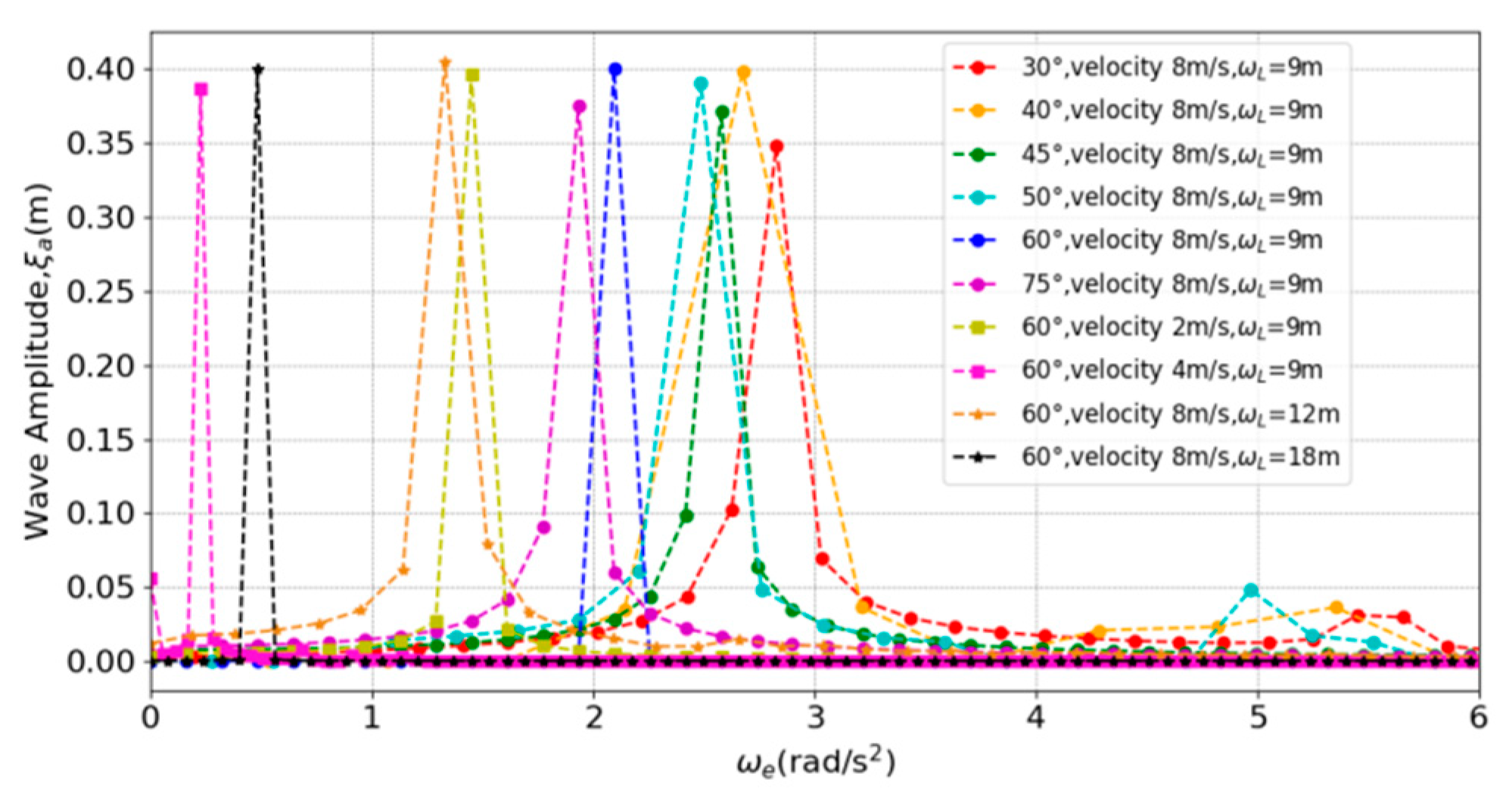
4.2. FFT Analysis of Wave Height

In order to intuitively present the encountered wave characteristics in different parameters and make comparisons of them, FFT is employed to gain insight into the linear dominant component in different cases.

From Figure 11, it is evident that two symmetric columns of waves will generate properties akin to regular waves, featuring a singular peak in their spectrum, with its amplitude roughly equivalent to the observed wave height in the temporal domain. Owing to the constraint of the time step in simulation monitoring and the fitting step in theoretical approximation, discrete Fourier transformation of the monitored wavelength curve will introduce some noise, resulting in slight dispersion of energy at each peak and, thus, marginally lower peak heights than anticipated. Nevertheless, the principal encounter frequencies indicated by the spectrum remain fairly accurate. This figure encompasses scenarios of USV navigating within symmetric intersecting waves with varying angles, wavelengths, and sailing velocities. The alterations in these parameters ultimately manifest as variations in the encounter frequencies, and it is necessary to note that the encounter frequencies shown in Figure 11 have been ordering by their absolute value. A discernible trend emerges from the graph: as the angle between the two waves increases, the encounter frequency gradually converges towards a lesser value; as the wavelength increases, the encounter frequency likewise shifts leftward. However, with the augmentation of the vessel’s sailing velocity, the magnitude of the encounter frequency does not exhibit a consistent pattern. Through the computation of the encounter frequency, it becomes apparent that when the sailing velocity (v) surpasses a certain threshold, the encounter frequency crosses zero and proceeds towards the negative half-axis, indicating a transition from following-wave to heading-wave sailing. Nevertheless, as the frequency transformed by the Fourier spectrum loses information regarding the relative motion of the waves, the consistent trend of encounter frequency displacement and sailing velocity alteration is not discernible within the positive half-axis of the Fourier spectrum.

4.3. USV Motions in Different Situations

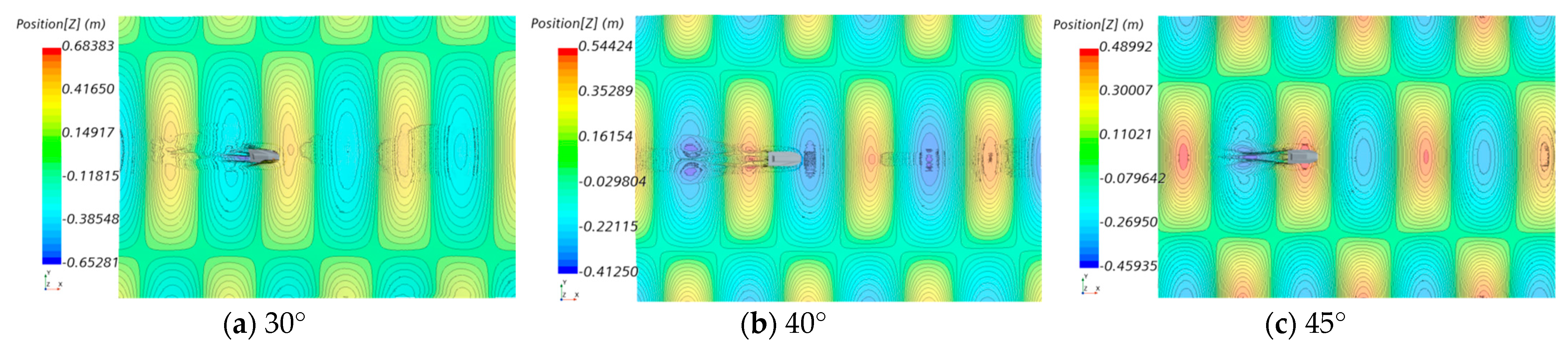
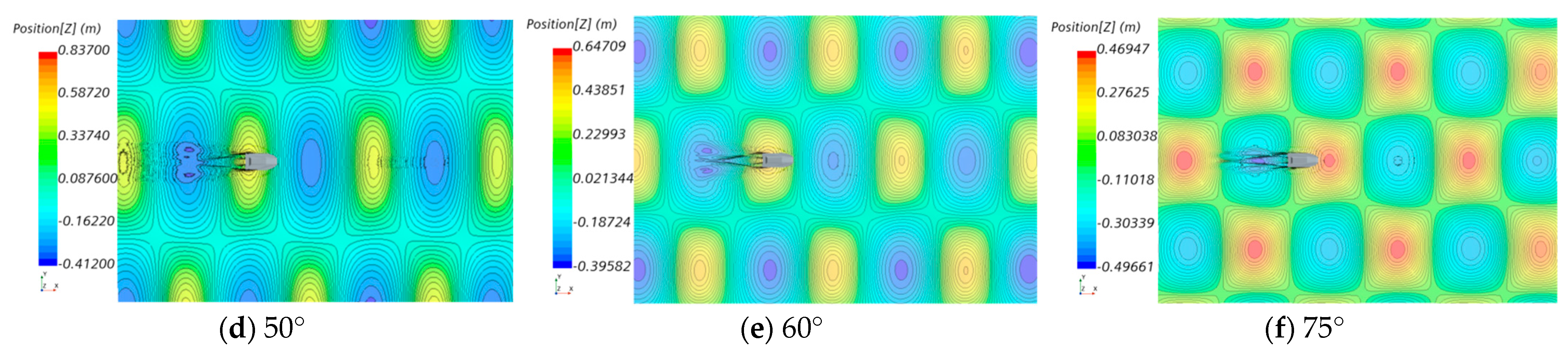
4.3.1. Different Inclination Angles of Intersecting Waves

The variation in the angle between the two superimposed waves results in differences in the concentration of wave energy along the centerline direction, leading to corresponding changes in the posture response of USVs traveling at the same speed. As a USV maneuvers between wave peaks and troughs, the difference between the superimposed wave’s velocity and its wave steepness constitutes varying input excitation signals for the USV, which can be modeled as an inertial system with delay. A comparison of monitoring data from different cases in the time domain is shown in Figure 12. In the various angle wave cases, the USV exhibits relatively small heave amplitude deviation but significant differences in pitch amplitude. This difference arises due to the actual encounter wavelengths of waves at different angles, while the theoretical amplitude values between peaks and troughs remain the same, causing variations in wave steepness. With changes in wave angles, it can be observed that the amplitude peak of pitch motion gradually increases, indicating a correlation between pitch motion and wave steepness. During the transition of pitch motion from bow down to stern down, there is a plateau period in pitch motion, which may relate to the simultaneous phase of wave troughs.

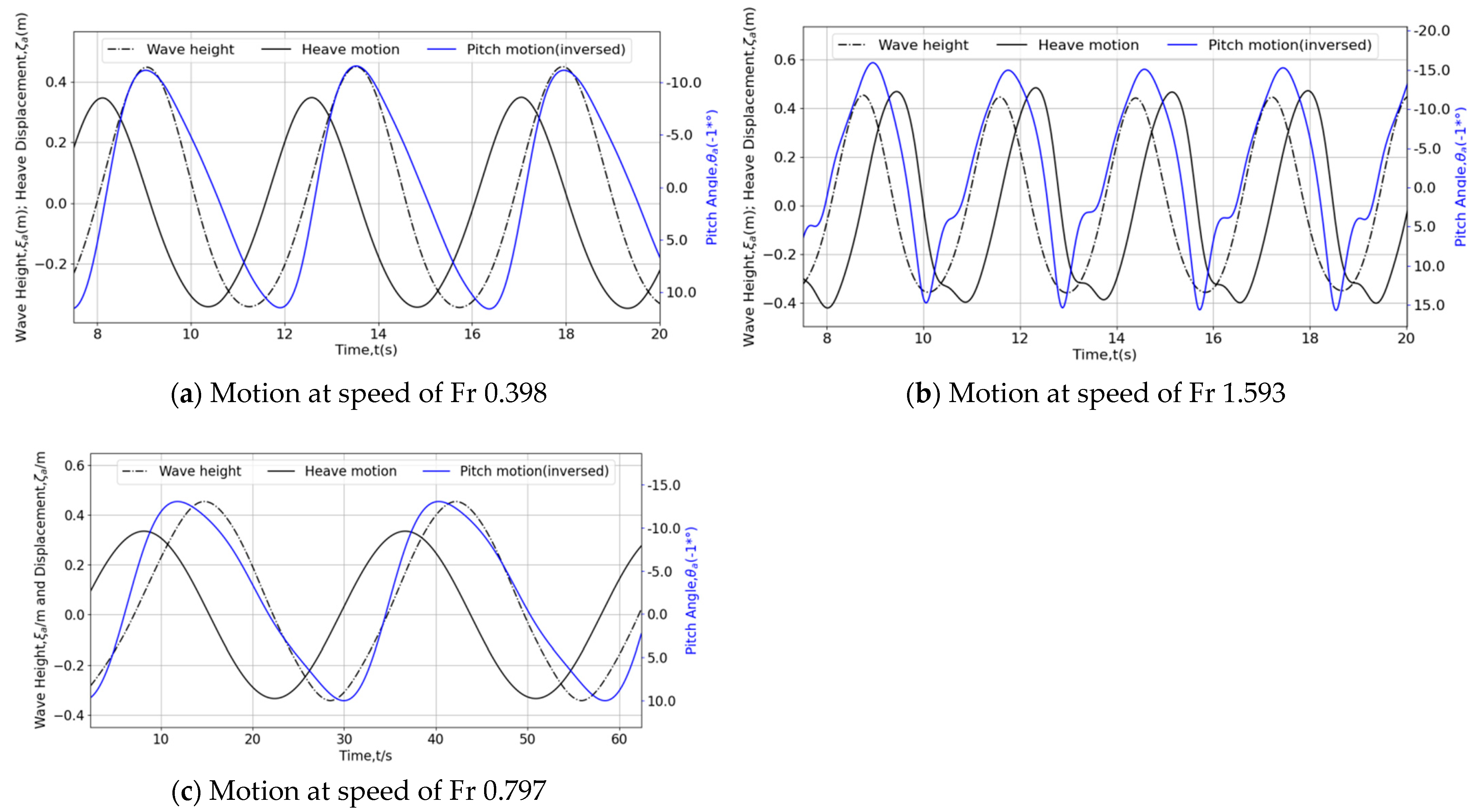
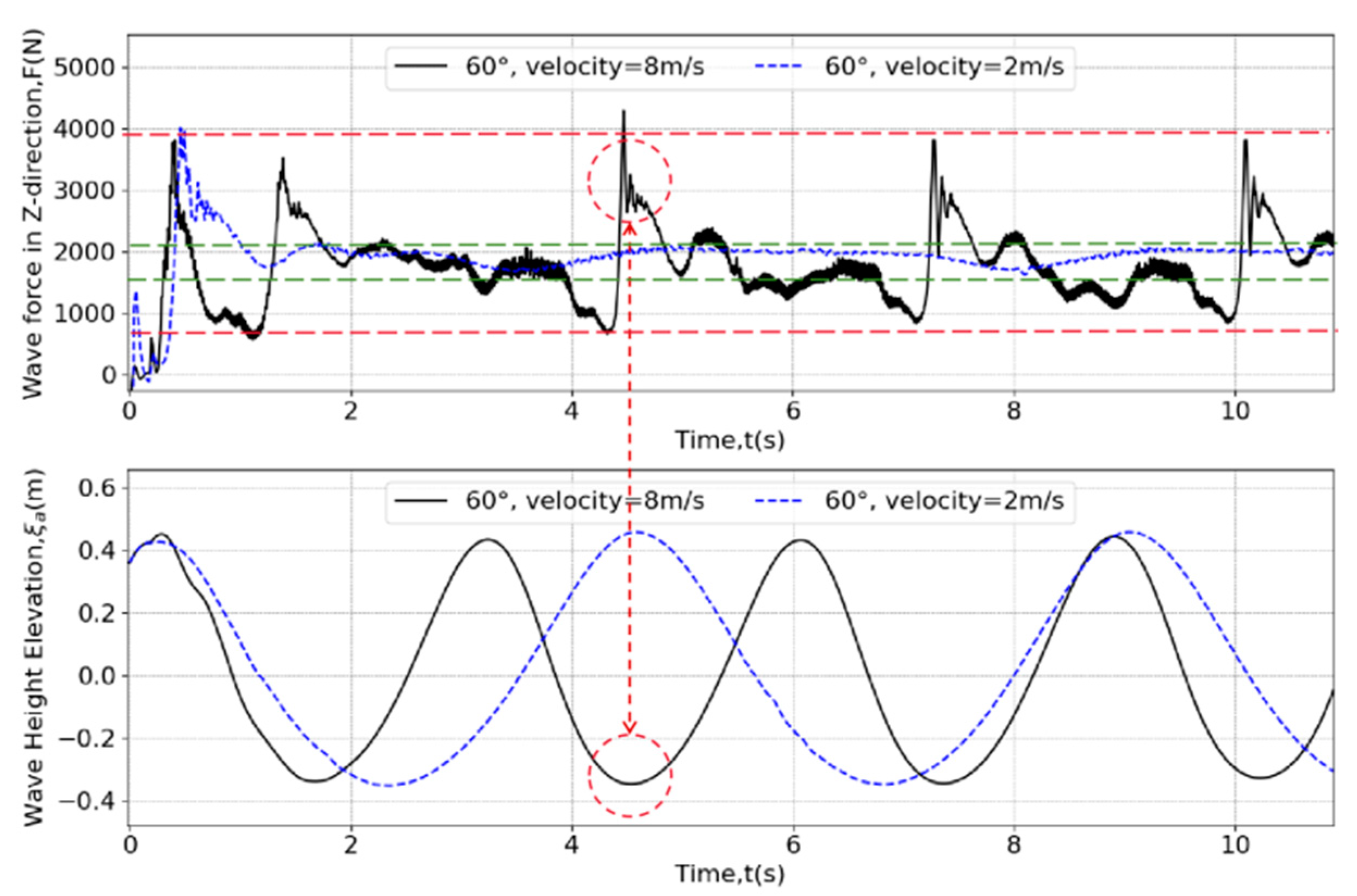
4.3.2. Different Navigating Speeds

Small-scaled USVs may face complicated planning motions when navigating in high speed, and the catamaran shape may introduce certain hydrodynamic characteristic. Stefano Zaghi et al. [85] studied the static hydrodynamic drag coefficient of catamarans at different Froude (Fr) numbers and varying hull spacings, revealing the causes of drag peaks by analyzing the relative movement between the wave troughs and the bow and stern positions of the USV. According to the patterns presented in the data from [85], as the sailing speed increases, the pitch angle of the catamaran in steady state exhibits a Z-shaped variation, while the heave volume shows a V-shaped variation. Honaryar A et al. [86] studied the interference effects between the two hulls of high-speed catamarans and explored the trends in resistance and pitch angle changes. They discovered a new phenomenon: the pitch angle range of high-speed catamarans with small clearances between the hulls decreases under static water conditions. They attributed this to the relative backward movement of the pressure center of the hull bottom, which also causes the planning phenomenon of high-speed USVs in static water, as mentioned by Faltinsen O M. 2005 [87]. Planning phenomena have been widely studied for high-speed ships, and some related simulation and optimization measures have been applied and validated through CFD and EXP [88,89,90,91,92].

In this paper, in order to investigate the distribution patterns of USV responses at different sailing speeds, this chapter examines the response motion and force of USV in escaping intersecting wave fields varying with different relative sailing speeds. Different free sailing speeds were designed to simulate the motion response of USVs intersecting regular waves. In the case of a wave intersecting angle of 60° (wave speed corresponding to Fr 0.982 at navigating direction), sailing speeds corresponding to Fr 0.398 and Fr 0.797 were chosen for comparison with the sailing speed corresponding to Fr 1.593, mentioned earlier. The motion and draft attitude of USV positioning at the middle of wave peaks and troughs and the distribution of hull pressure were observed from an underwater perspective. As shown in Figure 13, when the bow of the USV is at the wave trough and the stern is at the wave peak, the hull of Fr 1.593 is almost above the free surface, with only the inner rear edge of the twin side floats remaining submerged, and the pressure concentrated at the inner ridges reaches 4860 Pa. Under low-speed conditions, the pressure is evenly distributed across the bottom flat of the hull. The pressure is limited to 2100 Pa, much gentler than that in high-speed situations, mainly applied at the aft of the bottom flats and the front edges where the floating beams cut into the free surface. Under a speed corresponding to Fr 0.797, the slowest reaction occurs. There is a prolonged period when the USV rides on the crest and keeps that attitude navigating together with the wave trains. The major stress points are located near the front edges nearby the water surface, reaching 3600 Pa.

The comparison of elevation data obtained from wave measurement instruments attached to the USV at different sailing speeds is shown in Figure 14a–c, where the monitored pitch angle is inverted in sign, that is, with the unit of −1*°, for better consistency compared with other data. The encounter wave periods differ significantly at different encounter speeds. The relative velocity between wave speed and sailing speed determines the relative motion between the USV and the wave field, with the difference between absolute sailing speed and wave speed being a key influencing factor that correlates with the actual encounter frequency of waves at different USV speeds.

The encounter frequency between the USV and waves at different sailing speeds can also be reflected in the motion response. When the sailing speed is Fr 0.398, as shown in Figure 14a, the encounter frequency between the USV and waves is positive. This means that each wavelength of the waves gradually overtakes the ship’s side and propagates forward. As a result, peak wave height at the front of the ship lags behind the peak of the ship’s heave motion, and the amplitude of the USV’s heave motion is smaller than the wave height. This pattern can also be observed in Figure 13c, where the amplitudes of response motions remain at a similar level while every encounter period takes notably longer, which benefits from the slight difference in speed. On the other hand, when the sailing speed is Fr 1.593, as shown in Figure 13b, the encounter frequency between the USV and waves becomes negative. When the wave height reaches its peak in front of the USV, the hull is still in the climbing phase on the backside of the wave crest. After the wave crest completely passes over the center of gravity of the ship, the pitch angle of the USV begins to decrease. As the hull continues to move forward, the wetted surface of the hull gradually moves aft, causing the pressure center to shift aft. The combined wave force and gravity create a moment, resulting in a reduction in the trim angle of the USV. Only then does the heave motion of the USV begin to decrease. During this process, due to the strong inertia of the USV’s high-speed motion, the amplitude of the heave motion is greater than the height difference between the wave crest and trough.

Different speeds leads to different wave–ship interaction forms. Specifically, cases with Fr 0.398 and Fr 1.593 have similar amplitude of relative speed compared to wave speed. However, the former follows the waves, while the latter moves forward against them. A comparison of this two cases is valuable to in order to understand the differences in severity between positive and negative encounter scenarios. Wave forces loading on the ship–wave intersection part are inspected and shown in Figure 15, with wave height illustrated to indicate the moving stage. It is evident that in the force region of higher speed situation, an significant slamming peak takes place at the wave trough, as the red mark shows, and the force in the lower speed situation is limited nearby 2000 N, which is approximately the gravitational force value of USV, and remains relatively gentle throughout the monitoring process. The force only slightly decreases as the wave trough moves forward and slowly rebounds as the crest lifts the ship hull. It can be revealed that navigating at a higher positive speed against the wave generates more unsteady loading compared to traveling at a negative speed. This difference probably relates to the violent encounter process with the wave troughs and crests.

In the case of a sailing speed of Fr 0.398, the pressure monitoring cloud map is captured from the peak to the trough of the heave motion process, as shown in Figure 16. It can be observed that the pressure distribution forms an elliptical shape, which is consistent with the findings in [86]. The uniformly distributed pressure on the hull bottom during each critical phase of the waves profile is also beneficial to the steady navigational loading on the USV hull. Additionally, as each wave’s crest and trough pass through the hull from stern to bow, the pressure center at the bottom of the USV gradually moves backward. At 10.36 s, corresponding to a pitch angle of −2° in a floating state, the stern of the ship is immersed deeper, causing the pressure center to move backward.

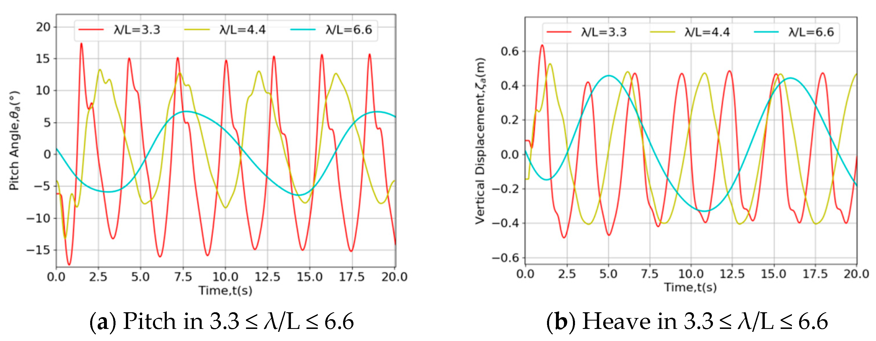
4.3.3. Different λ/L of Sub-Waves

At a sailing speed of Fr 1.593, the simulation of the superimposed wave field is conducted for different wavelengths of the sub-waves. The comparison of the wave surface elevation data at the bow of the USV is shown in the figure. The wavelength of the sub-waves also affects the wave number of the spatially superimposed waves, thus influencing the range of actual wave surface elevation variations.

Theoretically speaking, when the ship shuts down the thruster, the encounter speed at this wavelength is the traveling speed of the wave in the heading direction. However, in situations where two wave trains overlap at different inclination angles and different values of λ/L, creating a superposed wave, the intensity of the relative sea-keeping motion will be heavily influenced. There is an implied relationship among these parameters. To facilitate the discussion of the correlation between encounter frequency and the ratio of λ/L, we introduce the ship’s length, L, into Equation (14), deriving a new encounter frequency expression, Equation (17). By differentiating the encounter speed in Equation (17) with respect to the ratio λ/L, we obtain Equation (18).

For an inclination angle of 60°, the function curves are instantiated with the navigating speed of the USV set to 2 m/s, 4 m/s, and 8 m/s, respectively, as shown in Figure 17. By specifying the zero-point condition of Equation (18), it is evident that when the relationship in Equation (19) is satisfied, it indicates that as the ratio of λ/L increases, the encounter frequency rises. However, as the encounter frequency is negative, the absolute value of the encounter frequency experiences a rebound after an initial decline, and it is important to note that it is the absolute value of the encounter frequency that determines the encounter severity, whether the USV is overtaking crests or being caught up by them. This relationship is clearly visible in Figure 17. Before the curve intersects the zero line, the larger the λ/L, the milder the encounter tensity. After the encounter frequency turns positive, a larger λ/L leads to a larger encounter frequency, meaning that the waves behind come faster and push harder. This tendency does not reverse until the curve passes the critical point on the tuning line, which indicates that after this point, the encounter frequency declines as the ratio of λ/L continues to increase. Furthermore, when the USV is traveling at a lower speed, the drop in encounter frequency is more substantial. Moreover, by comparing the curves at different speed, it is significant to note that decelerating in an intersecting wave does not necessarily lead to a gentler encounter frequency, especially after the critical point. Opposite traveling waves may occur. Some data from CFD tests in this paper are marked in Figure 17, and they align well with the results of theoretical analysis.

$${\omega }_e=\sqrt{{\displaystyle \frac{2g\pi }{L}}}{rati{o}_{{\displaystyle \frac{\lambda }{L}}}}^{-{\displaystyle \frac{1}{2}}}-{\displaystyle \frac{2\pi v\cos \beta }{L}}{rati{o}_{{\displaystyle \frac{\lambda }{L}}}}^{-1}$$

(17)

$${\displaystyle \frac{\partial {\omega }_e}{\partial rati{o}_{\frac{\lambda }{L}}}}=-\sqrt{{\displaystyle \frac{g\pi }{2L}}}{rati{o}_{{\displaystyle \frac{\lambda }{L}}}}^{-{\displaystyle \frac{3}{2}}}+{\displaystyle \frac{2\pi v\cos \beta }{L}}{rati{o}_{{\displaystyle \frac{\lambda }{L}}}}^{-2}$$

(18)

$$rati{o}_{{\displaystyle \frac{\lambda }{L}}}<{\displaystyle \frac{8\pi v^2{\cos }^2\beta }{gL}}(rati{o}_{{\displaystyle \frac{\lambda }{L}}}>0)$$

(19)

As shown in Figure 18a, it can be observed that as the wavelength increases, the ship’s pitch range decreases and the period becomes longer. With the increase in wavelength, the wave period correspondingly lengthens. The ship’s motion, as a nonlinear response to the waves, exhibits a certain correlation in terms of its period. Therefore, the pitch period extends synchronously with the wave period. At the same time, the reduction in wave steepness significantly diminishes the ship’s pitching motion. As illustrated in Figure 18b, the ship’s heave motion curve becomes smoother, and the vertical oscillations commonly observed at wave troughs during high-speed navigation or under shorter wavelength waves tend to disappear.

5. Relevant Analysis of Response of USV in Wave

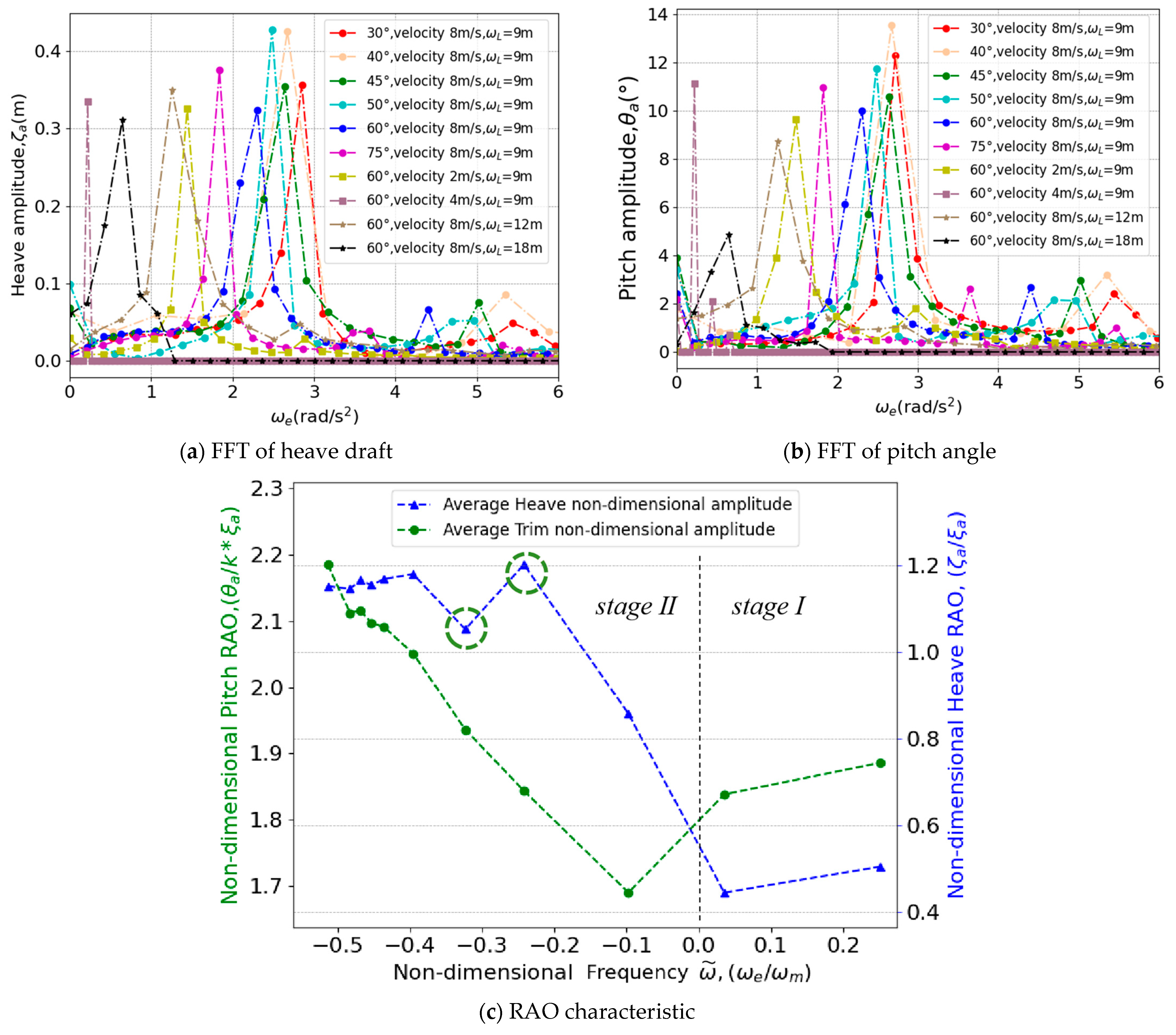
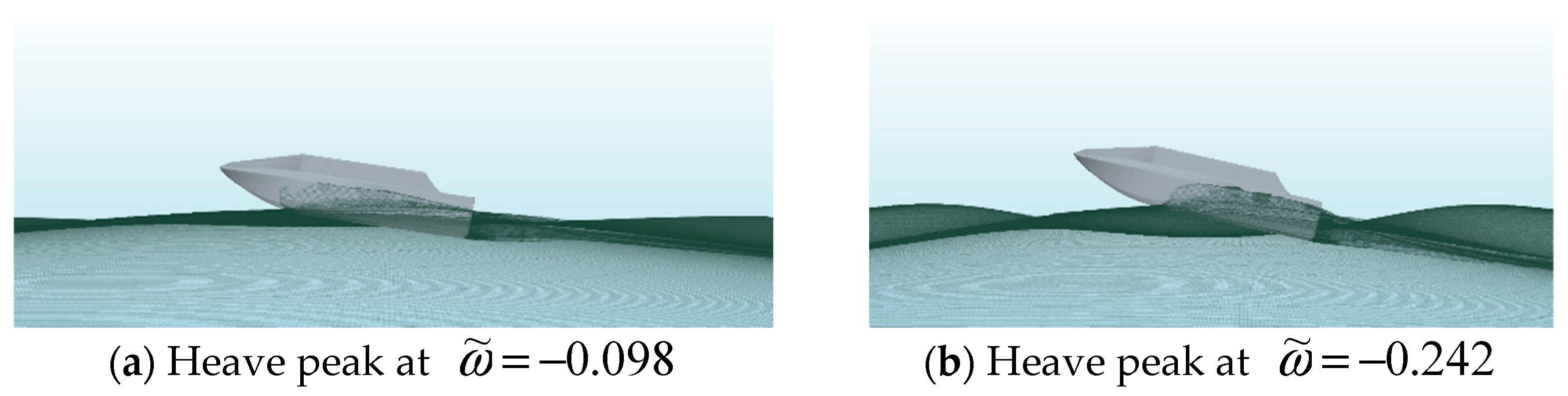
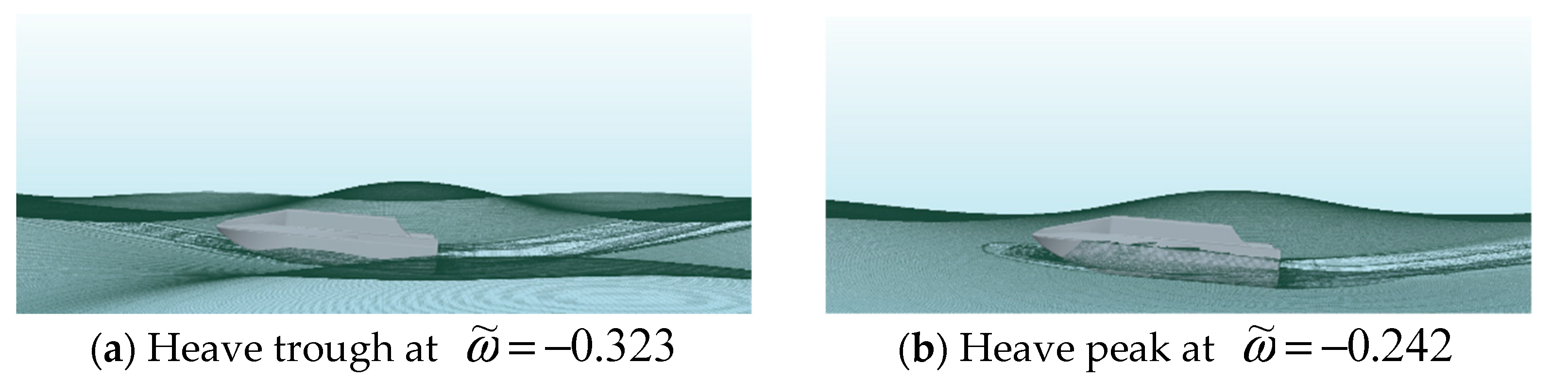
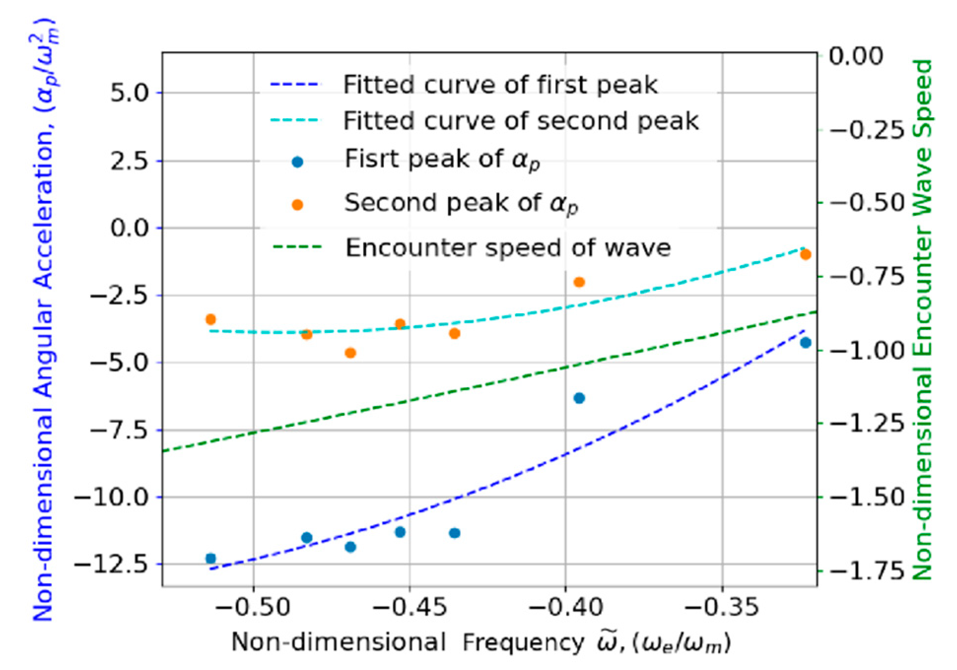
5.1. RAO Analysis of USV Motions with Encounter Frequency Perspective

FFT has been used to explore the sea-keeping motion of catamarans, as shown in [93]. In transitioning the USV’s surfing motion characteristics across scenarios with varying parameters to the encounter frequency perspective, we initially juxtapose the spectra of wave height, heave, and pitch motions. Subsequently, we conduct a frequency response analysis (RAO) for both heave and pitch motions, selecting eight motion cycles with closely aligned response curves. To mitigate the influence of initial position disparities observed across diverse operational conditions, we compute the monitored amplitude for each cycle as half the difference between the maximal and minimal motion amplitudes. Finally, we compute the mean of these monitored amplitudes across the eight cycles, excluding the extreme values.

The frequencies are multiplied by a coefficient to express them as circular frequencies. As shown in Figure 19a, the amplitude frequency of the heave motion matches the encountered wave frequency, but the magnitudes are marginally lower than the wave amplitudes at lower frequencies cases. Larger vertical heave happens more in ${\omega }_e=2~3$ rad/s, and minor peaks of motion spectrum plot are detected at higher frequencies, which reveals a minor perturbation faster than the main period during the motion. In Figure 19b, it can be observed that there is a smallest trim angle peak in the λ = 18 m case, i.e., λ/L = 6.6. Nevertheless, the pitch angle response characteristics in the relatively lower speed and shorter wavelength cases do not appear to be mild. To further reveal the underlying pattern of heave and pitch response, respond amplitude operators (RAOs) are applied below.

As Figure 19c shows, in the RAO analysis, as the nondimensional encounter frequency decreases, the average amplitude initially declines in Stage Ι and then subsequently rebounds in Stage ΙΙ after the encounter frequency becomes negative, which is transited to heading waves rather than following waves. Heave motion amplitude is highly influenced by the upper lifting caused by the crest and the deepened draft as it descends into the trough of waves. As the encounter waves intensify, the upper motion may be strengthened but the draft below the free surface may diminish. This is especially true as the navigating speed increases, leading to a decrease in draft due to the planning effect of the catamaran. These two opposing functions may cause some oscillations in the RAO characteristics, and with the increase in the absolute encounter frequency, the extreme heave motion of the USV becomes close to the value of 1.16 times the wave amplitude. While the general trend in Stage ΙΙ is consistent with the rising trend of encounter frequency, there are two minor turning points observed in Stage ΙΙ in the heave RAO curves at $\tilde{\omega }=-0.242$ and $\tilde{\omega }=-0.323$, which are highlighted with dashed-line circles.

We extract representative snapshots in the two cases mentioned above and the case of nondimensional encounter frequency $\tilde{\omega }=-0.098$ as well, and make some comparisons, as outlined below. In the process of oscillation shown in Figure 20a,b, there is a notable increase in the upper motion at wave crests in the latter case. Concurrently, when encountering low frequencies, the draft of USV remains relatively unchanged at the wave troughs. Hence, the overall amplitude of the heave motion temporarily increases with the rising waves, leading to the first turning point in heave RAO.

Compared with Figure 20b, a decrease in the height of the bow wave is observed in Figure 20a. This trend correlates with the reduction in displacement at the troughs of the USV. In Figure 21b, the USV exhibits a deeper sink, with pronounced wave formation on both sides, leading to waves cresting over the port side deck. Conversely, in the case shown in Figure 21a, the USV experiences a shallower draft, resulting in a relatively lower heave motion amplitude and the second turning point of heave motion.

Subsequently, as the nondimensional encounter frequency rises, the USV encounters a stronger wave, and the lifting angle reaches a maximum together with the draft slightly shrinking. The RAO characteristic maintains a stable level.

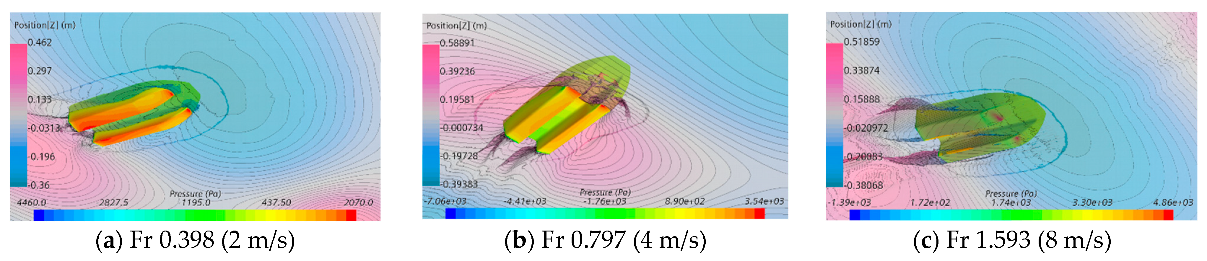
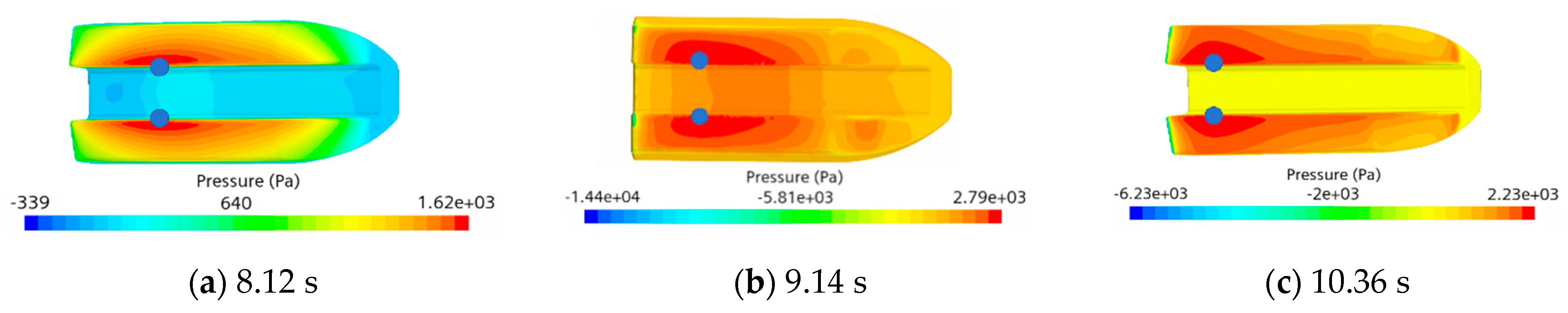
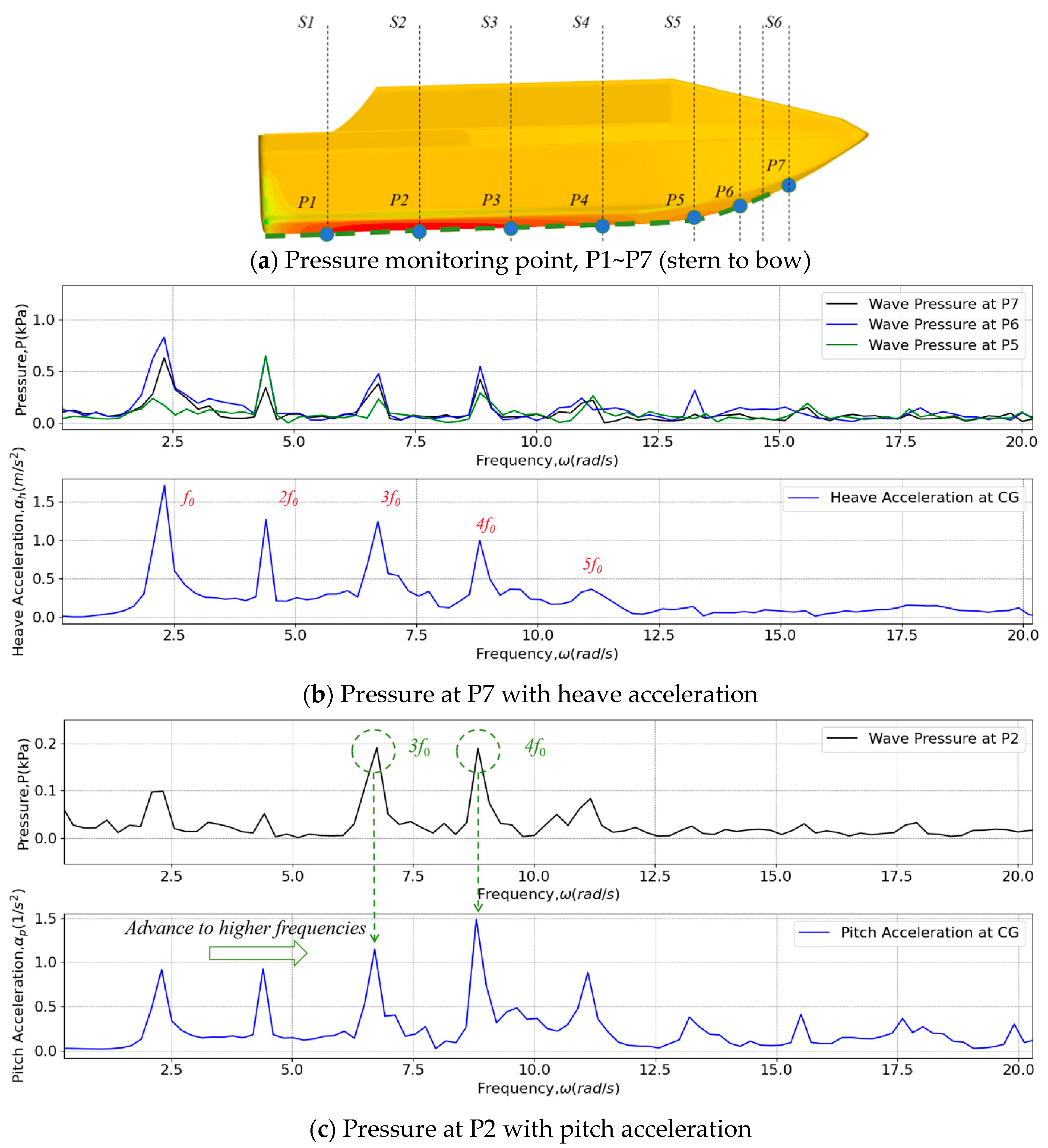
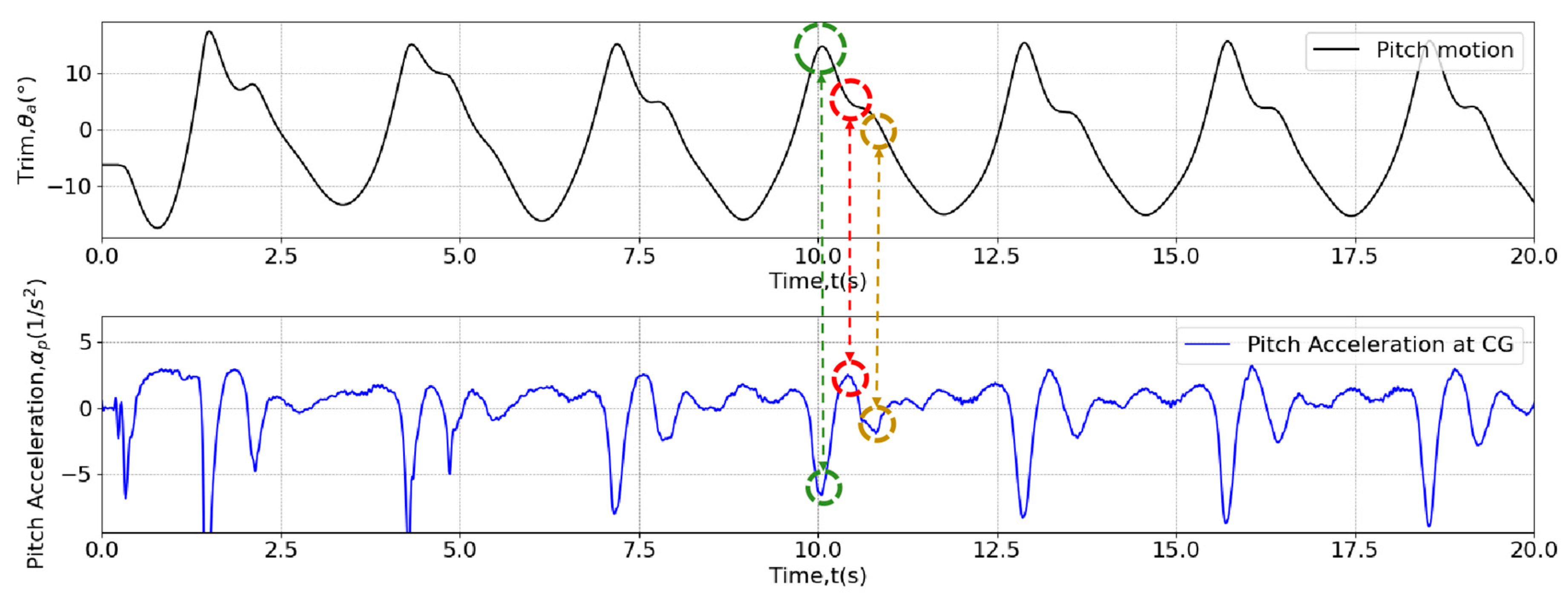
5.2. Relevant Analysis Between Pressure and Vertical Acceleration

To explore the relationship between pressure and the sea-keeping motion of a USV, seven pairs of monitoring points are symmetrically arranged at the bottom of two beams and an average pressure is calculated for each pair of symmetry probes, as shown in Figure 22a. To be specific, P1~P5 are located at the intersections of inner edges and station S1~S5, with a spacing of 0.4 m between each station. Additionally, P6, P7 are placed 0.2 m and 0.4 m forward of this arrangement, respectively.

To investigate the underlying patterns in the nonlinear response of the USV, an FFT transformation is applied to the pressure data under the conditions of a 60° inclination angle, a navigating speed of 8 m/s, a wavelength ratio of λ/L = 3.3, and, equally, an encounter frequency of ${\omega }_e=-2.32$ rad/s. The transformed curves are shown in Figure 22b,c. The data reveal that in the frequency characteristics of the two vertical accelerations, the harmonic spectral lines spread at integer multiples of the encounter frequencies. Moreover, the dominant frequency in the pitch acceleration motion slightly shifts toward higher values compared to that in heave. Additionally, the pressure loading at P5~P7 shows a strong relevance with the feature of heave motion acceleration. This suggests that the heave motion may be directly influenced by the pressure loading in the front region of the two beams, which resists the primary lifting effect of the encounter waves while increasing hydrodynamic pressure. In addition, the processing of pitch frequency lines matches well with the pressure characteristic curve at the P2 position, indicating that the pitching severity probably reaches a maximum when the pressure at the P2 position reaches its peak.

5.3. Severity Analysis of Vertical Pitch Response in Different Stages

As shown in Figure 23, in each cycle of the acceleration curve, there are three main peaks of interest. The first peak, the largest one, occurs when the hull of the ship is thrown upward by a wave crest and falls back to the trough. The rapid pitching angular velocity of the hull is counteracted by a tremendous slamming force, resulting in a significant negative instantaneous pitching angular acceleration. The second peak occurs when the hull is located at the trough, gradually restoring balance from a bow-down attitude. As the hull transitions from bow-down to stern-down, the center of buoyancy shifts aft beyond the center of gravity, causing the longitudinal pitching moment to become positive. This results in a brief descent of the bow, followed by the encounter with a new wave crest, which exacerbates the stern-down motion. The pitching angular acceleration also transitions to a negative direction, favoring the stern-down motion. The third acceleration peak appears shortly before the next encounter cycle.

$$c_{\mathrm{encounter}\mathrm{wave}}={\displaystyle \frac{\lambda \csc \frac{\theta }{2}}{-2\pi {\left(\omega -v\cos \frac{\theta }{2}{g}^{-1}{\omega }^2\right)}^{-1}}}$$

(20)

It can be hypothesized that the slamming process during the angular motion is induced by the encounter crest depth, which is associated with the actual wavelength and the encounter period of the wave. These factors are related to the synergistic effect of various elements, including wavelength, navigation speed, and inclination angles. A theoretical formula, as shown in Equation (20), illustrates the relationship between encounter wave speed and encounter frequency in symmetry-intersecting waves with different inclination angles and wavelengths. To reveal the trend of how angular acceleration changes with the encounter wave speed, the corresponding curve is displayed in Figure 24.

Obviously, the magnitude of the first acceleration peak is larger. To explore the characteristics of this acceleration peak and better understand the effects of intersecting waves at different angles on the cruising motion of USV, the angular acceleration of the pitch motion is compared, as shown in the figure. As the angle increases, ranging from 30° to 75°, the encounter wave frequency decreases, leading to a prolonged encounter wave period. Additionally, as the wavelength increases, the steepness of the encountered wave decreases, reducing the severity of the USV’s response to wave resistance.

Consequently, the peak angular acceleration of the pitch motion decreases accordingly. It can be observed that the second peak follows a similar pattern to the first, despite the fact that their magnitudes differ from each other. Also, the encountered wave speed, indeed, decreases in the same manner, which closely matches the trend of becoming mild of both peaks of pitch acceleration. We can draw the inference that there is a nearly positive relationship between the relative wave speed and the severity of pitch motion. When the travel period and amplitude of each individual wave in the composed wave train are fixed, this variable can represent the steepness of wave spectrum. Any parameter change that can lead to an increase in relative traveling speed of the USV and the wave itself makes it highly possible to result in a sharp response on the USV. This linear relationship can be applied in the dynamic regulation algorithm of a USV, allowing for smoother and milder control for safety considerations.

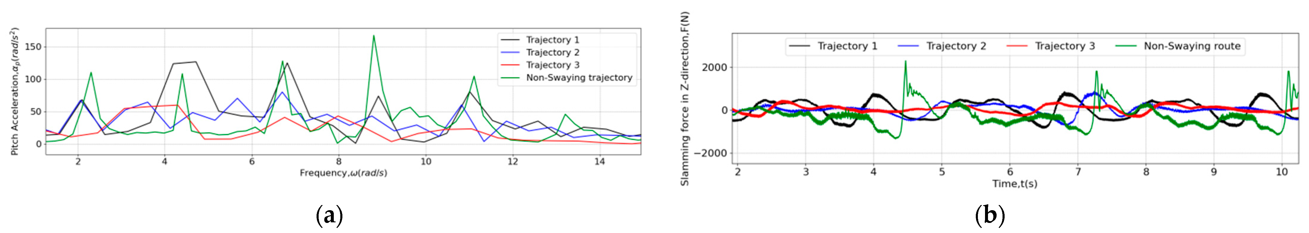
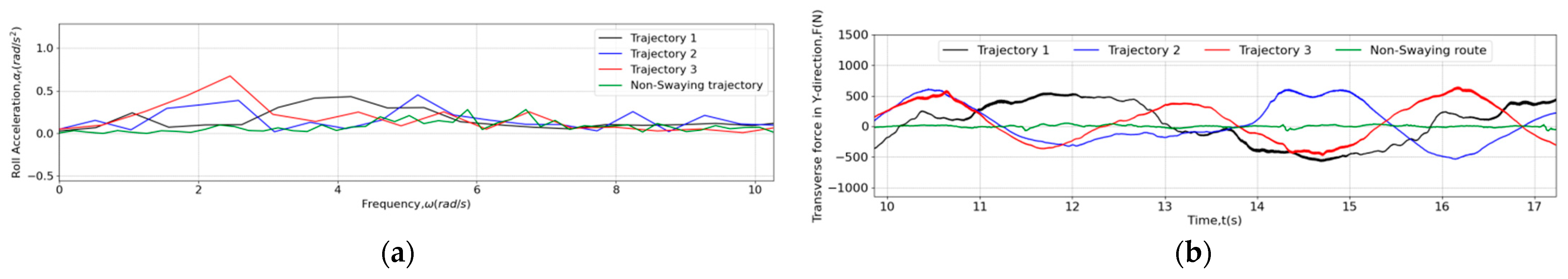
6. Swaying Tests with PMM

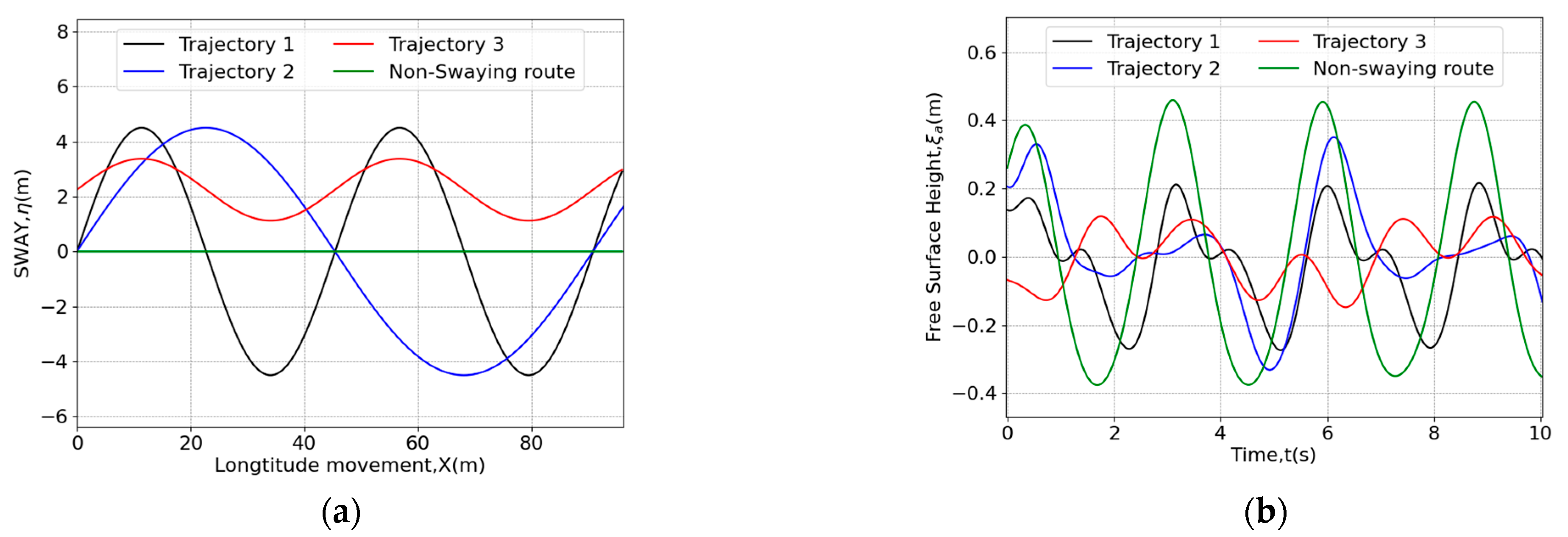
6.1. Encountered Waves of Different Swaying Routes

In order to find a navigating trajectory with a milder response, pure swaying tests are designed in this chapter, simulating the motion response under continuously changing directions. Unlike navigating in a constant direction, pure swaying tests allow the USV to sail with a sinusoidal yaw angle change, and different snapshots during an entire period are shown in Figure 25. The actual wave strength encountered depends on lateral moving amplitude and period. Three routes are visualized in Figure 26a and listed in

Table 7. Parameters of the PMM swaying trajectory.

Routes	Longitude Towing Speed, v0/m × s−1	Lateral Moving Amplitude, y0/m	Swaying Period, T/s	Initial Lateral Position Offset from Original Route, b0/m
Trajectory 1	8	4.5	2.82	0
Trajectory 2	8	4.5	5.64	0
Trajectory 3	8	1.125	2.82	2.25

, in which periods are set up according to 1 and 1/2 times the encountered frequency for a case where $\theta =0.098°,v=8\mathrm{m}/\mathrm{s},\mathrm{L}=9m$, and amplitudes are set in consideration of minimizing the encountered wave height, aiming to pass through the stagnation line in the region as much as possible, rather than through the crests and trough. It can be clearly observed that the USV detours away from the crests, which is proven by Figure 25b. As shown in Figure 26b, the wave elevation amplitudes of Trajectory 1~3 decreased to varying degrees, as expected. Meanwhile, the polychromatic property also appears in the encountered waves, tuning out the influence of the transverse effect of intersecting waves.

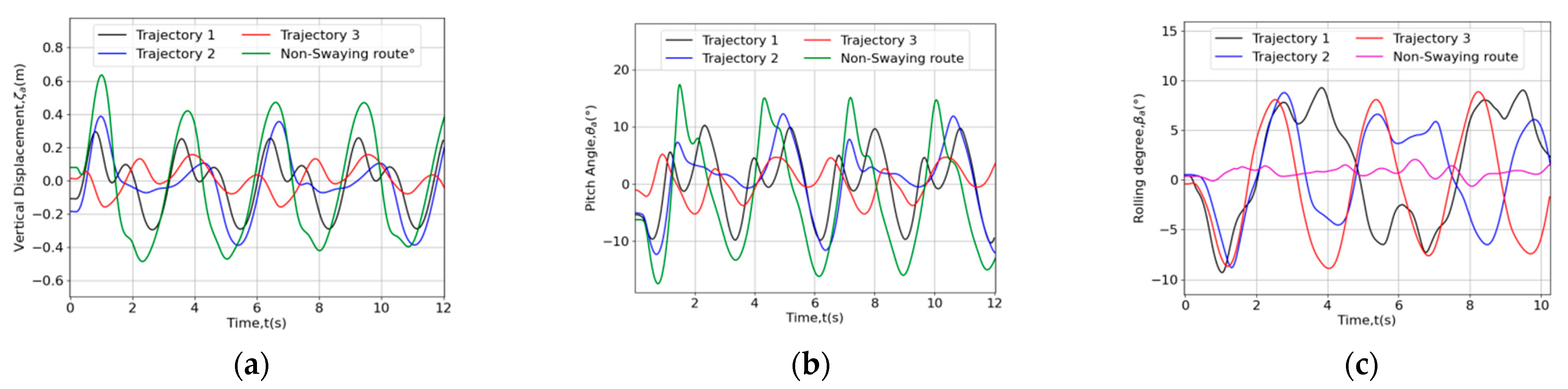
6.2. Sea-Keeping Response Comparisons

Taking vertical motion response as the primary concern, we can see from Figure 27 that the largest amplitude of Trajectories 1~3 decreases following the same trend of encountered wave height. Trajectory 3 appears to have the mildest vertical response amplitude, which is further verified by Figure 28a. The acceleration in this case shows lower amplitude across all frequencies and a relatively even slamming curve, indicating smooth interaction with the waves. However, the rolling responses amplify significantly during all this swaying process. As revealed by Figure 27c and Figure 29b, some monochromatic periodicity is present in the transverse loading, and the transverse motion is actually much larger compared to the original nonswaying route. We selected a pressure snapshot from the Trajectory 3 case at t = 11.5 s, where the transverse loading reaches a negative extreme, and a snapshot in the nonswaying, where the load is primarily vertical, as shown in Figure 30. It can be observed that when the USV passes through the centerline of crest and trough, the wave approaching from the left side hits the rear starboard of the port side, causing lateral slamming. This results in a high-pressure band-like region forming at the lower middle of the port side. At the same time, with the hull separating from the edge of the previously superimposed crest, the draft of the starboard side decreases, and the positive pressure zone on the starboard side diminishes and shifts backward. Negative pressure zones appear on both sides at the front edge of the beams and below the starboard side, as the next superimposed wave trough is soon encountered. As for the vertical negative pressure regions at the bow and stern, they appear as a result of the wave diffraction process, becoming the major cause of wave resistance. Predictably, as the yaw angle continues to turn to the right, the USV will gradually sail into the wave trough ahead. During this process, the rolling angle will gradually increase due to the imbalance of transverse loading on both sides of the USV.

In summary, Trajectories 2 and 3 show a significant decrease in pitch response acceleration by lengthening the swaying period and offsetting away from the peak–trough line, The latter helps to ease the vertical slamming loads throughout the process. Additionally, the lateral amplitudes of all three swaying tests were designed to diminish the encountered wave height, which proved effective. However, side effects from deviating from the original straightforward route also exist. Specifically, rolling motion amplitudes may increase substantially, and lateral stability could be compromised as a result of the conversion of the slamming force from the vertical direction to the transverse direction. Moreover, substantial pressure impacts acting on both sides of the hull, in addition to the bottom, may cause damage to the side structure.

7. Conclusions

A CFD study predicting the sea-keeping behavior of unmanned surface vehicles under the influence of intersecting waves was conducted. By conducting a series of CFD simulation experiments considering navigating speed, wavelength, and the inclination angles of the intersecting waves, this study analyzed the wave loads and ship reaction intensity. Some conclusions were drawn, as follows.

(1) A narrower inclination, ranging from 75° to 30°, generally leads to a more severe encounter situation, which increases the pitching amplitude. The amplitude of the encounter frequency follows a decrease–increase–decrease trend as λ/L increases. The same navigating speed in a smaller λ/L may cause an increase in the encounter frequency, but in a longer wave, it may result in an intense inverse frequency, which does not necessarily alleviate the sea-keeping response. The crucial factor is the encountered speed. A negative encountered wave speed leads to shallower draft and violent pitch slamming, but allows a USV to effectively move out of the waves field. When the encounter speed turns positive, the ship is passively tossed by the faster wave, which causes a dangerous heeling-forward situation, weakening maneuverability and propulsion. Thus, the ideal situation for the ship is to sail slightly faster than the wave does, although it is challenging for a USV to autonomously perceive the wave period.

(2) As the absolute magnitude of the encounter frequency increases, the amplitudes of the pitching response rise, and the heave motion tends to approach an extreme value of 1.16 times the wave amplitude. During this process, the increasing encounter speed leads to a decrease in the draft at the wave trough and a rise at the wave crest, both of which influence the trends of the heave amplitude changing under different encounter conditions. Intense heaving generates wave loading on the front edges of the two beams of the catamaran, while the pitching intensity is closely related to the loading on the rear middle area behind the center of gravity.

(3) By studying the developing trends of the top two sharp peaks of pitch acceleration, a positive relationship between the relative wave speed and the severity of vertical motion was found. The RAO showed that the two peaks generally follow two patterns but follow the same trend as the encounter wave speed. In the domain discussed in this paper, the encounter speed in two trains of waves with fixed amplitude and traveling period can accurately describe the steepness and criticality of the encounter situation.

(4) Proper trajectory selection may help decrease the severity of the vertical wave response by detouring away from the crest and trough lines and adjusting the swaying frequency according to the even times of encounter periods. However, with the decrease in vertical loading, significant transverse loading will occur on both sides of the USV hull, inevitably introducing a rolling response. Even when navigating near the stationary line of intersecting waves, where wave height remains consistent, transverse imbalance may occur.

8. Future

For a USV navigation strategy in an intersecting wave field, a self-adapting speed controlling mode seems to be beneficial for safer navigation while the dynamic effects still remain unknown. This also relies on the propulsion efficiency of the USV’s propeller in such a complicated wave field. Further simulation work on these topics holds great prospect.

References

1. Liu, Z.; Zhang, Y.; Yu, X.; Yuan, C. Unmanned surface vehicles: An overview of developments and challenges. Annu. Rev. Control 2016, 41, 71–93. [Google Scholar] [CrossRef]
2. Wang, W.; Pakozdi, C.; Kamath, A.; Bihs, H. Representation of 3-h Offshore Short-Crested Wave Field in the Fully Nonlinear Potential Flow Model REEF3D::FNPF. J. Offshore Mech. Arct. Eng. 2022, 144, 041902. [Google Scholar] [CrossRef]
3. Xiang, G.; Xiang, X.; Datla, R. Numerical study of a novel small waterplane area USV advancing in calm water and in waves using the higher-order Rankine source method. Eng. Appl. Comput. Fluid Mech. 2023, 17, 2241892. [Google Scholar] [CrossRef]
4. Townsend, J. The Application of Computational Fluid Dynamics to the Modelling and Design of High-Speed Boats; Swansea University: Swansea, UK, 2021. [Google Scholar]
5. Sun, H.; Jing, F.; Jiang, Y. Zou, J; Zhuang, J; Ma, W. Motion prediction of catamaran with a semisubmersible bow in wave. Pol. Marit. Res. 2016, 23, 37–44. [Google Scholar] [CrossRef]
6. Diez, M.; Broglia, R.; Durante, D.; Campana, E.F.; Stern, F. Validation of highfidelity uncertainty quantification of a high-speed catamaran in irregular waves. In Proceedings of the 13th International Conference on Fast Sea Transportation, FAST, Washington, DC, USA, 2–4 September 2015; pp. 1–4. [Google Scholar]
7. Diez, M.; Broglia, R.; Durante, D.; Campana, E.F.; Stern, F. Statistical validation of a high-speed catamaran in irregular waves. In Proceedings of the 31st Symposium on Naval Hydrodynamics, Monterey, CA, USA, 11–16 September 2016; pp. 11–16. [Google Scholar]
8. Xie, J. Investigation on nonlinear interactions of bidirectional waves. Dalian Univ. Technol. 2021, 003915. [Google Scholar]
9. Cavaleri, L.; Bertotti, L.; Torrisi, L.; Bitner-Gregersen, E.; Serio, M.; Onorato, M. Rogue waves in crossing seas: The Louis Majesty accident. J. Geophys. Res. Ocean 2012, 117. [Google Scholar] [CrossRef]
10. Adcock, T.A.A.; Taylor, P.H.; Yan, S.; Ma, Q.; Janssen, P. Did the Draupner wave occur in a crossing sea? Proc. R. Soc. A Math. Phys. Eng. Sci. 2011, 467, 3004–3021. [Google Scholar] [CrossRef]
11. Jiao, J.; Huang, S.; Soares, C.G. Numerical investigation of ship motions in cross waves using CFD. Ocean Eng. 2021, 223, 108711. [Google Scholar] [CrossRef]
12. Huang, S.; Jiao, J.; Chen, C. CFD prediction of ship seakeeping behavior in bi-directional cross wave compared with in uni-directional regular wave. Appl. Ocean Res. 2021, 107, 102426. [Google Scholar] [CrossRef]
13. Chen, Z.; Zhao, N.; Zhao, W.; Xia, J. Numerical prediction of seakeeping and slamming behaviors of a trimaran in short-crest cross waves compared with long-crest regular waves. Ocean Eng. 2023, 285, 115314. [Google Scholar] [CrossRef]
14. Petrova, P.G.; Guedes Soares, C. Distributions of nonlinear wave amplitudes and heights from laboratory generated following and crossing bimodal seas. Nat. Hazards Earth Syst. Sci. 2014, 14, 1207–1222. [Google Scholar] [CrossRef]
15. Sabatino, A.D.; Serio, M. Experimental investigation on statistical properties of wave heights and crests in crossing sea conditions. Ocean Dyn. 2015, 65, 707–720. [Google Scholar] [CrossRef]
16. Ocaña-Blanco, D.; Castañeda-Sabadell, I.; Souto-Iglesias, A. CFD and potential flow assessment of the hydrodynamics of a kitefoil. Ocean Eng. 2017, 146, 388–400. [Google Scholar] [CrossRef]
17. Kandasamy, M.; Ooi, S.K.; Carrica, P.; Stern, F.; Campana, E.F.; Peri, D.; Osborne, P.; Cote, J.; Macdonald, N.; de Waal, N. CFD validation studies for a high-speed foil-assisted semi-planing catamaran. J. Mar. Sci. Technol. 2011, 16, 157–167. [Google Scholar] [CrossRef]
18. Amani, S. Numerical and Experimental Analysis of the Wind Forces Acting on a High-Speed Catamaran; University of Tasmania: Hobart, Australia, 2019. [Google Scholar]
19. Haase, M.; Zurcher, K.; Davidson, G.; Binns, J.R.; Thomas, G.; Bose, N. Novel CFD-based full-scale resistance prediction for large medium-speed catamarans. Ocean Eng. 2016, 111, 198–208. [Google Scholar] [CrossRef]
20. Phan, K.M.; Sadat, H. CFD study of extreme ship responses using a designed wave trail. Ocean Eng. 2023, 268, 113178. [Google Scholar] [CrossRef]
21. Carrica, P.M.; Fu, H.; Stern, F. Computations of self-propulsion free to sink and trim and of motions in head waves of the KRISO Container Ship (KCS) model. Appl. Ocean Res. 2011, 33, 309–320. [Google Scholar] [CrossRef]
22. Yu, L.; Wang, S.; Ma, N. Study on wave-induced motions of a turning ship in regular and long-crest irregular waves. Ocean Eng. 2021, 225, 108807. [Google Scholar] [CrossRef]
23. Wang, W.; Bihs, H.; Kamath, A.; Arntsen, Ø.A. Multi-directional irregular wave modelling with CFD. In Proceedings of the Fourth International Conference in Ocean Engineering (ICOE2018), Chennai, India, 18–21 February 2018; Springer: Singapore, 2019; Volume 1, pp. 521–529. [Google Scholar]
24. Li, J.; Wang, Z.; Liu, S. Experimental study of interactions between multi-directional focused wave and vertical circular cylinder, part II: Wave force. Coast. Eng. 2014, 83, 233–242. [Google Scholar] [CrossRef]
25. Liu, S.; Ong, M.C.; Obhrai, C.; Seng, S. CFD simulations of regular irregular waves past a horizontal semi-submerged cylinder. J. Offshore Mech. Arctic. Eng. 2017, 140. [Google Scholar]
26. Zhang, L.; Zhang, J.; Shang, Y. A practical direct URANS CFD approach for the speed loss and propulsion performance evaluation in short-crested irregular head waves. Ocean Eng. 2021, 219, 108287. [Google Scholar] [CrossRef]
27. Kim, D.; Tahsin, T. CFD-based hydrodynamic analyses of ship course keeping control and turning performance in irregular waves. Ocean Eng. 2022, 248, 110808. [Google Scholar] [CrossRef]
28. Judge, C.; Mousaviraad, M.; Stern, F.; Lee, E.; Fullerton, A.; Geiser, J.; Schleicher, C.; Merrill, C.; Weil, C.; Morin, J.; et al. Experiments and CFD of a high-speed deep-V planing hull–part II: Slamming in waves. Appl. Ocean Res. 2020, 97, 102059. [Google Scholar] [CrossRef]
29. Wu, C.; Zhou, D.; Gao, L.; Miao, Q. CFD computation of ship motions and added resistance for a high speed trimaran in regular head waves. Int. J. Nav. Archit. Ocean. Eng. 2011, 3, 105–110. [Google Scholar] [CrossRef]
30. Nowruzi, L.; Enshaei, H.; Lavroff, J.; Kianejad, S.S.; Davis, M.R. CFD simulation of motion responses of a trimaran in regular head waves. Int. J. Marit. Eng. 2020, 162, A1. [Google Scholar] [CrossRef]
31. Wang, S.; Guedes Soares, C. Review of ship slamming loads and responses. J. Mar. Sci. Appl. 2017, 16, 427–445. [Google Scholar] [CrossRef]
32. Ardeshiri, S.; Mousavizadegan, S.H.; Kheradmand, S. Virtual simulation of PMM tests independent of test parameters. Brodogr. Int. J. Nav. Archit. Ocean Eng. Res. Dev. 2020, 71, 55–73. [Google Scholar] [CrossRef]
33. Liu, J.; Chua, K.H.; Taskar, B.; Liu, D.; Magee, A.R. Virtual PMM captive tests using OpenFOAM to estimate hydrodynamic derivatives and vessel maneuverability. Ocean Eng. 2023, 286, 115654. [Google Scholar] [CrossRef]
34. Zhu, Z.; Kim, B.S.; Wang, S.; Kim, Y. Study on Numerical PMM Tests in Incident Waves. In Proceedings of the 37th International Workshop on Water Waves and Floating Bodies, Giardini Naxos, Italy, 10–13 April 2022. [Google Scholar]
35. Ma, C.; Hino, T.; Ma, N. Numerical investigation of the influence of wave parameters on maneuvering hydrodynamic derivatives in regular head waves. Ocean Eng. 2022, 244, 110394. [Google Scholar] [CrossRef]
36. Ma, C.Q.; Ma, N.; Gu, X.C. Numerical simulation of PMM tests of a container ship in regular following waves. In Sustainable Development and Innovations in Marine Technologies; CRC Press: Boca Raton, FL, USA, 2019; pp. 197–204. [Google Scholar]
37. Zhu, Z.; Kim, B.S.; Wang, S.; Kim, Y. Observation of the Wave Effect on Ship Manoeuvring Coefficients Based on Numerical PMM Approach. In Proceedings of the ISOPE International Ocean and Polar Engineering Conference, Online, 5–10 June 2022; p. ISOPE-I-22-345. [Google Scholar]
38. The Specialist Committee on Uncertainty Analysis. In Proceedings of the 26th International Towing Tank Conference 2011, Rio de Janeiro, Brazil, 28 August–3 September 2011.
39. Reynolds, O. IV. On the Dynamical Theory of Incompressible Viscous Fluids andthe Determination of the Criterion. Philos. Trans. R. Lond. 1895, 186, 123–164. [Google Scholar]
40. Shih, T.H.; Liou, W.W.; Shabbir, A.; Yang, Z.; Zhu, J. A new k-ϵ eddy viscosity model for high reynolds number turbulent flows. Comput. Fluids 1995, 24, 227–238. [Google Scholar] [CrossRef]
41. Shih, T.H.; Liou, W.W.; Shabbir, A.; Yang, Z.; Zhu, J. A new k-epsilon eddy viscosity model for high Reynolds number turbulent flows: Model development and validation. NASA Technical Memorandum 1994, 106721, 1–30. [Google Scholar]
42. Kim, D.; Song, S.; Sant, T.; Demirel, Y.K.; Tezdogan, T. Nonlinear URANS model for evaluating course keeping and turning capabilities of a vessel with propulsion system failure in waves. Int. J. Nav. Archit. Ocean Eng. 2022, 14, 100425. [Google Scholar] [CrossRef]
43. Terziev, M.; Tezdogan, T.; Demirel, Y.K.; Villa, D.; Mizzi, S.; Incecik, A. Exploring the effects of speed and scale on a ship’s form factor using CFD. Int. J. Nav. Archit. Ocean Eng. 2021, 13, 147–162. [Google Scholar] [CrossRef]
44. Ferziger, J.H.; Perić, M.; Street, R.L. Computational Methods for Fluid Dynamics; Springer: Berlin/Heidelberg, Germany, 2019. [Google Scholar]
45. Ohmori, T. Finite-volume simulation of flows about a ship in maneuvering motion. J. Mar. Sci. Technol. 1998, 3, 82–93. [Google Scholar] [CrossRef]
46. Ohmori, T.; Miyata, H. Oblique tow simulation by a finite-volume method. J. Soc. Nav. Archit. Jpn. 1993, 1993, 27–34. [Google Scholar] [CrossRef]
47. Shabana, A.A. Computational Dynamics; John Wiley & Sons: Hoboken, NJ, USA, 2009. [Google Scholar]
48. Benek, J.A.; Steger, J.L.; Dougherty, F.C. Chimera: A Grid-Embedding Technique; Arnold Engineering Development Center, Air Force Systems Command, United States Air Force: Tullahoma, TN, USA, 1986. [Google Scholar]
49. Field, P.L. Comparison of RANS and Potential Flow Force Computations for the ONR Tumblehome Hullfrom in Vertical Plane Radiation and Diffraction Problems. Va. Tech. 2013. [Google Scholar]
50. ITTC Specialist Committee. Recommended procedures and guidelines-Practical Guidelines for Ship CFD Applications. In Proceedings of the 26th International Towing Tank Conference, Rio de Janeiro, Brasil, 5–10 September 2010. [Google Scholar]
51. ITTC Manoeuvring Committee. Final report and recommendations to the 28th ITTC. In Proceedings of the 28th International Towing Tank Conference, Wuxi, China, 17–22 September 2017. [Google Scholar]
52. Sezen, S.; Cakici, F. Numerical prediction of total resistance using full similarity technique. China Ocean Eng. 2019, 33, 493–502. [Google Scholar] [CrossRef]
53. Li, H.; Zhao, N.; Zhou, J.; Chen, X.; Wang, C. Uncertainty Analysis and Maneuver Simulation of Standard Ship Model. J. Mar. Sci. Eng. 2024, 12, 1230. [Google Scholar] [CrossRef]
54. Morabito, M.; Park, J.; van Rijsbergen, M. Quality systems group. In Proceedings of the 28th International Towing Tank Conference 2017, Wuxi, China, 17–22 September 2014. [Google Scholar]
55. Gerhardt, F.; Young, J.; Minoura, M.; Bouscasse, B.; Hermundstad, O.A.; Nam, B.W.; Duan, W. Procedures and Guidelines. 2024. Available online: https://www.ittc.info/media/11894/75-02-07-025.pdf (accessed on 10 November 2024).
56. De Luca, F.; Mancini, S.; Miranda, S.; Pensa, C. An extended verification and validation study of CFD simulations for planing hulls. J. Ship Res. 2016, 60, 101–118. [Google Scholar] [CrossRef]
57. Roache, P.J. Verification and Validation in Computational Science and Engineering; Hermosa: Albuquerque, NM, USA, 1998. [Google Scholar]
58. Ec¸a, L.; Vaz, G.; Hoekstra, M. Code verification, solution verification and validation in RANS solvers. In Proceedings of the International Conference on Offshore Mechanics and Arctic Engineering, Shanghai, China, 6–11 June 2010; Volume 49149, pp. 597–605. [Google Scholar]
59. Chen, Y.; Xu, S.; Shi, J.; Liu, X.; Hou, G. Hydrodynamic performance of small unmanned catamaran based on STAR-CCM+. Chin. J. Ship Res. 2023, 18, 73–82. [Google Scholar]
60. Islam, H.; Soares, C.G. Uncertainty analysis in ship resistance prediction using OpenFOAM. Ocean Eng. 2019, 191, 105805. [Google Scholar] [CrossRef]
61. Tasai, F. Damping force and added mass of ships heaving and pitching (continued). In Reports of Research Institute for Applied Mechanics; Research Institute for Applied Mechanics, Kyushu University: Fukuoka, Japan, 1960. [Google Scholar]
62. Keuning, J.A. A calculation method for the heave and pitch motions of a hydrofoil boat in waves. Int. Shipbuild. Prog. 1979, 26, 217–232. [Google Scholar] [CrossRef]
63. Gerritsma, J. Some notes on the calculation of pitching and heaving in longitudinal waves. Int. Shipbuild. Prog. 1956, 3, 255–264. [Google Scholar] [CrossRef]
64. Katayama, T.; Ikeda, Y. A Study on Coupled Pitch and Heave Porpoising Instability of Planing Craft. J.-Kansai Soc. Nav. Archit. Jpn. 1997, 226, 227. [Google Scholar]
65. Katayama, T.; Hinami, T.; Ikeda, Y. Longitudinal motion of a super high-speed planing craft in regular head waves. In Proceedings of the 4th Osaka Colloquium on Seakeeping Performance of Ships, Osaka, Japan, 17–21 October 2000; pp. 214–220. [Google Scholar]
66. Irannezhad, M.; Eslamdoost, A.; Kjellberg, M.; Bensow, R.E. Investigation of ship responses in regular head waves through a Fully Nonlinear Potential Flow approach. Ocean Eng. 2022, 246, 110410. [Google Scholar] [CrossRef]
67. Barrass, B.; Derrett, C.D.R. Ship Stability for Masters and Mates, 6th ed.; Butterworth-Heinemann: Oxford, UK, 2006. [Google Scholar]
68. Biran, A.; López-Pulido, R. Ship Hydrostatics and Stability; Butterworth-Heinemann: Oxford, UK, 2003. [Google Scholar]
69. Tupper, E.C.; Rawson, K.J. Basic Ship Theory, 5th ed.; Volume 2: Ship Dynamics and Design; Butterworth-Heinemann: Oxford, UK, 2001. [Google Scholar]
70. Oogushi, M. Ship Engineering Theory, 10th ed.; Kaibundo Shuppan: Tokyo, Japan, 1999. [Google Scholar]
71. Boйткунский, Я.И.; Першиц, Р.Я.; Титoв, И.А. Справoчник пo теoрии кoрабля. Л: Судпрoмгиз. 1960; 228. [Google Scholar]
72. Turkyilmazoglu, M. Maximum wave run-up over beaches of convex/concave bottom profiles. Cont. Shelf Res. 2022, 232, 104610. [Google Scholar] [CrossRef]
73. Komar, P.D.; Gaughan, M.K. Airy wave theory and breaker height prediction. Coast. Eng. 1972, 1973, 405–418. [Google Scholar]
74. Le Roux, J.P. An extension of the Airy theory for linear waves into shallow water. Coast. Eng. 2008, 55, 295–301. [Google Scholar] [CrossRef]
75. Le Roux, J.P. Profiles of fully developed (Airy) waves in different water depths. Coast. Eng. 2008, 55, 701–703. [Google Scholar] [CrossRef]
76. Wang, L.; Liu, W.; Lai, Z. Simulation method for simulating wave disturbance signals. Ship Eng. 2002, 4, 23–27. [Google Scholar]
77. Hsu, J.R.C.; Tsuchiya, Y.; Silvester, R. Third-order approximation to short-crested waves. J. Fluid Mech. 1979, 90, 179–196. [Google Scholar] [CrossRef]
78. Hsu, H.C.; Chen, Y.Y.; Hsu, J.R.C.; Tseng, W.-J. Nonlinear water waves on uniform current in Lagrangian coordinates. J. Nonlinear Math. Phys. 2009, 16, 47–61. [Google Scholar] [CrossRef]
79. Waseda, T.; Tamura, H.; Kinoshita, T. Freakish sea index and sea states during ship accidents. J. Mar. Sci. Technol. 2012, 17, 305–314. [Google Scholar] [CrossRef]
80. Zhang, Z.; Li, X.-M. Global ship accidents and ocean swell-related sea states. Nat. Hazards Earth Syst. Sci. 2017, 17, 2041–2051. [Google Scholar] [CrossRef]
81. Hammack, J.L.; Henderson, D.M.; Segur, H. Progressive waves with persistent two-dimensional surface patterns in deep water. J. Fluid Mech. 2005, 532, 1–52. [Google Scholar] [CrossRef]
82. Elgar, S. Waves in oceanic and coastal waters. Oceanography 2007, 20, 133–135. [Google Scholar] [CrossRef]
83. Liu, Z.; Fang, K. Two-layer Boussinesq models for coastal water waves. Wave Motion 2015, 57, 88–111. [Google Scholar] [CrossRef]
84. Daripa, P.; Dash, R.K. A class of model equations for bi-directional propagation of capillary–gravity waves. Int. J. Eng. Sci. 2003, 41, 201–218. [Google Scholar] [CrossRef]
85. Zaghi, S.; Broglia, R.; Di Mascio, A. Analysis of the interference effects for high-speed catamarans by model tests and numerical simulations. Ocean Eng. 2011, 38, 2110–2122. [Google Scholar] [CrossRef]
86. Honaryar, A.; Ghiasi, M.; Liu, P.; Honaryar, A. A new phenomenon in interference effect on catamaran dynamic response. Int. J. Mech. Sci. 2021, 190, 106041. [Google Scholar] [CrossRef]
87. Faltinsen, O.M. Hydrodynamics of High-Speed Marine Vehicles; Cambridge University Press: Cambridge, UK, 2005. [Google Scholar]
88. Bessho, M.; Komatsu, M.; Anjoh, M. On motions of a high speed planning boat in regular head sea. J. Soc. Nav. Archit. Jpn. 1974, 1974, 109–120. [Google Scholar] [CrossRef]
89. Sun, H.; Huang, D.; Zou, J. Experimental investigation on resistances from stepped trimaran-planing boats. Huazhong Univ. Sci. Technol. 2012, 40, 86–89. [Google Scholar]
90. Kim, Y.S.; Hwang, S.K. A Study on Air Resistance and Greenhouse Gas Emissions of an Ocean Leisure Planning Boat. J. Korean Soc. Mar. Environ. Energy 2013, 16, 202–210. [Google Scholar] [CrossRef]
91. Shen, H.; Xiao, Q.; Zhou, J.; Su, Y.; Bi, X. Design of hydrofoil for the resistance improvement of planing boat based on CFD technology. Ocean Eng. 2022, 255, 111413. [Google Scholar] [CrossRef]
92. Park, K.; Kim, D.J.; Kim, S.Y.; Seo, J.; Suh, I.; Rhee, S.H. Effect of waterjet intake plane shape on course-keeping stability of a planing boat. Int. J. Nav. Archit. Ocean Eng. 2021, 13, 585–598. [Google Scholar] [CrossRef]
93. Jinglei, Y.; Hanbing, S.; Xiaowen, L.; Wu, D. Experimental study on wave motion of partial air cushion supported catamaran. Int. J. Nav. Archit. Ocean Eng. 2023, 15, 100525. [Google Scholar] [CrossRef]
Figure 1. Intersecting waves observed in the Qiantang River estuary.
Jmse 13 00083 g001
Figure 2. The three-dimensional model. (a) The three-dimensional model. (b) The simplified three-dimensional model front view. (c) The original USV hull.
Jmse 13 00083 g002
Figure 3. Virtual towing tank dimension configuration. (a) Virtual towing tank side view. (b) Virtual towing tank back view.
Jmse 13 00083 g003
Figure 4. Comparison of grid schemes (a) Scheme A, (b) Scheme B, (c) Scheme C, and (d) Wave elevations in different mesh schemes.
Jmse 13 00083 g004
Figure 5. Ship model testing environment.
Jmse 13 00083 g005
Figure 6. Comparison of linear solution and high-ordered solution.
Jmse 13 00083 g006
Figure 7. Intersecting wave field area. (a) Griding—overlapping grids. (b) Initialization—wave surface.
Jmse 13 00083 g007
Figure 8. Physical field conditions around the hull. (a) Water–air interface condition. (b) Distribution of y+ on hull surface. (c) Magnitude of velocity in water region.
Jmse 13 00083 g008
Figure 9. Superposition of intersecting waves with different inclination angles (a) 30°, (b) 40°, (c) 45°, (d) 50°, (e) 60°, (f) 75°.
Jmse 13 00083 g009aJmse 13 00083 g009b
Figure 10. Free surface height elevation of intersecting waves of cases (a) 30°, (b) 45°, (c) 60°, (d) 75°, (e) 0.39 ≤ Fr ≤ 1.58, (f) 3.3 ≤ λ/L ≤ 6.6.
Jmse 13 00083 g010
Figure 11. FFT of encountered waves elevations.
Jmse 13 00083 g011
Figure 12. (a) Pitch in 30–75°, (b) Heave in 30–75° USV motion monitoring in intersecting regular waves at various angles.
Jmse 13 00083 g012
Figure 13. Wave elevation and pressure profile at different speeds at the middle of a crest and a trough.
Jmse 13 00083 g013
Figure 14. Wave height elevation at different navigating speeds.
Jmse 13 00083 g014
Figure 15. Wave force in two extreme cases.
Jmse 13 00083 g015
Figure 16. Snapshots of pressure at the bottom of USV beams at different stages (a) 8.12 s, (b) 9.14 s, (c) 10.36 s.
Jmse 13 00083 g016
Figure 17. Transition between encounter speed and λ/L.
Jmse 13 00083 g017
Figure 18. Vertical motion in different wavelengths ratio (a) Pitch in 3.3 ≤ λ/L ≤ 6.6, (b) Heave in 3.3 ≤ λ/L ≤ 6.6.
Jmse 13 00083 g018
Figure 19. Spectrum and RAO analysis of USV vertical motion (a) FFT of heave draft, (b) FFT of pitch angle, (c) RAO characteristic.
Jmse 13 00083 g019
Figure 20. Profile of USV motion at wave crests.
Jmse 13 00083 g020
Figure 21. Profile of USV motion at wave troughs.
Jmse 13 00083 g021
Figure 22. FFT of pressure monitoring data (a) Pressure monitoring point, P1~P7 (stern to bow), (b) Pressure at P7 with heave acceleration, (c) Pressure at P2 with pitch acceleration.
Jmse 13 00083 g022
Figure 23. Angular acceleration characteristics.
Jmse 13 00083 g023
Figure 24. RAO of pitch acceleration.
Jmse 13 00083 g024
Figure 25. Surface profile in Trajectory 1 (a) Snapshot 1, (b) Snapshot 2, (c) Snapshot 3, (d) Snapshot 4, (e) Snapshot 5.
Jmse 13 00083 g025
Figure 26. Trajectory of swaying tests. (a) Routes of USV PMM tests. (b) Encountered wave height ahead of the USV.
Jmse 13 00083 g026
Figure 27. Vertical response characteristics comparison. (a) Heave motion response. (b) Pitch motion response. (c) Roll motion response.
Jmse 13 00083 g027
Figure 28. Vertical characteristics. (a) Pitch acceleration frequency. (b) Vertical wave slamming sequence.
Jmse 13 00083 g028
Figure 29. Transverse characteristics. (a) Roll acceleration frequency. (b) Transverse wave loading sequence.
Jmse 13 00083 g029
Figure 30. Snapshots in Trajectory 3 and nonswaying trajectory. (a) Surface snapshot in Trajectory 3. (b) Pressure in Trajectory 3. (c) Pressure in nonswaying trajectory.
Jmse 13 00083 g030