AFF-LightNet: A Lightweight Ship Detection Architecture Based on Attentional Feature Fusion

Abstract

Efficient mobile detection equipment plays a vital role in ensuring maritime safety, and accurate ship identification is crucial for maritime traffic. Recently, the most advanced learning-based methods have markedly improved the accuracy of ship detection, but these models often face huge challenges on resource limited mobile devices due to their large size and high computational requirements. Thus, we propose a lightweight ship detection network based on attentional feature fusion, called AFF-LightNet. To enhance the fusion of multi-scale features and semantically inconsistent features, we introduce iterative attentional feature fusion (IAFF) into the proposed neck network, improving the efficiency of feature fusion by introducing a multi-scale channel attention module. Also, deep and cross network version 2 (DCNv2) is replaced by Convolution (Conv) in the backbone network to further improve the detection accuracy of the proposed network. It enhances the spatial sampling position in convolution and Region of Interest (Rol) pooling by introducing offsets. Moreover, a lightweight convolution GhostConv was introduced into the head network to reduce the number of parameters and computation cost. Last, Scalable Intersection over Union (SIOU) loss was leveraged to improve the convergence speed of the model. We conduct extensive experiments on the publicly available dataset SeaShips and compare it with existing methods. The experimental results show that compared with the standard YOLOv8n, the improved network has an average accuracy of 98.8%, an increase of 0.4%, a reduction of 1.9 G in computational complexity, and a reduction of 0.19 M in parameter count.

1. Introduction

Ship target detection, as an indispensable real-time monitoring technology in the marine environment, has shown high application value and practical significance in multiple key fields. Specifically, this technology plays a crucial role in improving the safety and efficiency of port operations, optimizing the response speed of maritime emergency rescue, ensuring absolute safety of ship navigation, and promoting sustainable management of fishery resources. Early ship detection methods mainly relied on manual observation and radar technology. The former mainly depended on crew members to identify the position and motion status of ships through naked eyes or optical equipment, while the latter detected the position and motion status of ships by emitting electromagnetic waves and receiving reflected waves. These methods relied on subjective human judgment and were influenced by factors such as lighting and weather. Since computer vision technology has advanced, cameras and image manipulation techniques have also begun to be applied to ship monitoring. Methods based on feature extraction and pattern recognition have gradually emerged, but their accuracy and robustness in complex marine environments are very limited. In recent years, significant progress has been made in ship detection methods based on deep learning, especially those based on convolutional neural network models, which greatly improve the accuracy and effectiveness of ship detection and make significant contributions to the cause of maritime traffic safety.

Deep learning-based detection methods reduce reliance on manual labor and automatically achieve end-to-end detection. Two categories can be distinguished between deep learning-based algorithms: two-stage algorithms and single-stage algorithms. The two-stage algorithm mainly consists of two main stages: candidate region generation and candidate region classification. Its common algorithms include R-CNN, Fast R-CNN, Faster R-CNN [1,2,3], etc. Although two-stage algorithms have great advantages in accuracy and reliability, their algorithm speed is slow and cannot achieve real-time monitoring purposes. In addition, they also have high requirements for computing resources and pose certain challenges for detecting small or dense targets. The single-stage algorithm directly predicts the position and category of targets in the image without the need for candidate region generation and classification, with high real-time performance and simple network structure. The common algorithms mainly include SSD [4], YOLO [5,6,7,8,9,10,11] series, etc. Although single-stage algorithms have lower computational complexity than two-stage algorithms, they are still not lightweight enough for mobile devices with limited marine resources.

To solve the problem of a lack of lightweight many lightweight CNN network models have been proposed one after another, such as MobileNetV1, V2, V3 [12,13,14] ShuffleNetV1, V2 [15,16], etc. MobileNetV3 mainly achieves lightweighting by combining a depthwise separable convolution and neural structure search, while ShuffleNetV2 enables the network lightweighting through shuffling operations and equalization of channel width. These networks can effectively make the model lightweight, while their lightweighting are commonly achieved at the expense of model detection accuracy. Moreover, the marine environments are generally complicated, such as obstructed ships or complex backgrounds, so their detection results still cannot meet monitoring requirements.

In addition, the clarity of images captured by maritime surveillance systems is often affected by factors such as occlusion, lighting, and shooting angles. This low-quality image poses a huge challenge to the monitoring of maritime traffic safety. It becomes particularly difficult to accurately identify ships under poor visual conditions. Also, the complex and ever-changing marine environment requires extremely high equipment requirements for monitoring systems. Large equipment cannot work continuously and stably in edge operations, and the real-time performance of systematic data transmission is poor, which cannot meet the needs of maritime traffic safety. In order to meet this demand, some common practices sacrifice detection performance to achieve lightweight requirements, but this process weakens the detection accuracy of ships due to the loss of feature details.

To ensure its detection speed and accuracy, improvements and optimizations are made on the basis of YOLOv8. Firstly, deformable convolution is used, which can adaptively adjust the shape and sampling position of the convolution kernel. Secondly, attention mechanism-based feature fusion is introduced to enhance feature fusion. Then, in terms of lightweight, GhostConv [17] convolution was used to reduce computational costs and parameter count through low-cost linear transformation. Finally, the SIOU [18] loss function was introduced to improve the convergence speed of the model. This model ensures its detection accuracy while achieving lightweight, making it suitable for resource limited offshore monitoring systems. And a large number of experiments were conducted on the optical image ocean ship dataset SeaShips7000 [19] to demonstrate the effectiveness of the proposed model. The main contributions of this article are as follows:

• We propose a lightweight network for maritime vessel detection by combining lightweight convolutional GhostConv with iterative attention feature fusion iAFF and DCNv2 convolution, which not only meets the requirements of detection accuracy but also reserves expected lightweight nature;
• The SIOU loss function is introduced in the model to ensure the convergence speed and detection accuracy of the model;
• Compared with other models, this model achieves a better balance between detection accuracy and model lightweight.

The rest of the work in this article is arranged as follows: In Section 2, the development history of YOLO series algorithms is reviewed; Section 3 elaborates on the proposed lightweight ship detection model based on feature fusion; Section 4 presents the experimental results on the SeaShips dataset; Section 5 provides a summary of this work.

2. Related Works

2.1. The YOLO Series

Joseph Redmon et al. suggested YOLOv1 [5] in 2016, with an astonishing detection speed of processing 45 images per second, meeting the requirements of real-time detection. However, it is not friendly to small object detection and localization. So, in 2017, Joseph Redmon et al. made significant improvements on YOLOv1 and proffer YOLOv2 [6], which referenced the K-means clustering method to focus on solving the problems of low target recall and low small object detection accuracy. However, in 2018, Redmon et al. replaced the original darknet-19 network with darknet-53 and presented a feature pyramid network based on YOLOv2 for multi-scale detection, giving birth to YOLOv3 [7]. This not only improves its detection accuracy but also ensures real-time detection performance. In 2020, Alexey Bochkovskiy et al. proposed YOLOv4 [8], which replaced darknet-53 [20] with CSP (Cross Stage Partial Connection)—Darknet53, and SPP [21] technology was introduced to significantly expand the model’s receptive field, enabling the capture and separation of more critical and important contextual features. In the same year, Glenn Jocher released YOLOv5, which was developed using PyTorch and employed various enhancement techniques to enhance its robustness. In addition, YOLOv5 also introduced the C3 module to achieve a lightweight effect on its model. Afterwards, many versions of the YOLO series were released, such as YOLOv7 [9], YOLOR [11], YOLOX [10], and so on. Until the release of YOLOv8 in 2023, it replaced the C3 module with the C2f module based on YOLOv5, which combined advanced features with contextual information, further reducing the complexity of the model. Compared to the C3 module, C2f has a richer gradient flow to meet the needs of models at different scales. Furthermore, YOLOv8 also adopts an anchor-free (anchor-free model) decoupling head, which helps the model reduce positioning errors and provide better recognition performance, improving the detection performance of the model. It not only supports omnidirectional visual AI tasks, including detection, segmentation, pose estimation, tracking, and classification, but also provides models at various scales to meet the needs of different scenes.

In the continuous evolution of object detection technology, many explorers have explored the applicability of the YOLO series to ship detection tasks. For example, Zhang et al. [22] proposed a ship object detection model based on the improved YOLOv5 algorithm, by using a bidirectional feature pyramid network and a coordinate attention technique, they were able to recognize ships more accurately; a ship detection method based on the YOLOX algorithm proposed by Liu et al. [23] improves the original model by introducing residual structures and CIOU loss functions; Wang et al. [24] proposed an enhanced YOLOv8 ship detection method based on multi-scale attention feature fusion. They integrated the asymptotic feature pyramid (AFPN) large selective kernel attention mechanism (LSK) and the fourth detection head into YOLOv8, dynamically adjusting its receptive field and enhancing the recognition representation of ships, greatly improving the performance of the model; Guo et al. [25] proposed a sea vessel detection target based on the YOLOv7 model, by integrating the lightweight architecture of MobileNetv1 and the innovative design of shallow feature fusion path, the performance of the object detection model has been significantly enhanced; Cheng et al. [26] proposed an improved lightweight ship detection model based on YOLOv8, which utilizes Faster-Net Block and EMA attention mechanism to balance lightweight and detection accuracy. Siddique et al. [27] proposed a novel scalar image with enhanced leakage enhancement. The image is preprocessed using Gaussian and Laplacian filters for image enhancement, and feature extraction is performed using CNN and Convolutional Autoencoder (CAE). The color intensity changes in the AE scalar image are mainly enhanced; Siddique et al. [28] designed a hybrid deep learning method by combining enhanced Fourier transform spectrogram with continuous wavelet transform and deep learning, which mainly ensures the safety and integrity of fluid transportation. Siddique et al. [29] proposed a method for detecting bearing faults by using vibration signals to obtain Mel transform scalar maps. By optimizing the Mel filter bank and FOX optimizer, the model achieved the best performance of high accuracy, high recall, and high F1 score.

2.2. Feature Fusion

Feature fusion plays a crucial role in object detection. Shallow features contain rich local details and edge information but lack semantic information, while deep features contain rich semantic information but lack local details and edge information. At this point, feature fusion strategy becomes crucial. Through feature fusion, feature maps from different levels can be fused together, allowing the target detector to better utilize information from different scales and semantic levels, thereby improving detection accuracy. There are generally three ways of feature fusion: (1) Cascading feature fusion, which mainly involves cascading feature maps from different levels and then fusing them through convolution; (2) Feature pyramid, which mainly involves constructing a pyramid network that includes feature maps of different scales, and then fusing information between different levels through convolution and other methods; (3) Attention mechanism, which mainly adjusts the weights of feature maps dynamically by adding attention mechanism, allowing the model to adaptively select fused features. Their typical representative modules include the CEDNet (Cascade Encoder Decoder Network) proposed by Zhang et al. [30] in 2023. It integrates different encoder–decoder structures to perform multiple scales feature fusion in the decoder, thereby improving the performance of the model; the BiFPN (Bilateral Feature Pyramid Network) [31] proposed by Google further improves the performance of feature fusion by introducing bidirectional and cross layer connections in the FPN [32]; the iAFF (Iterative Attention Feature Fusion) proposed by Yimian Dai et al. [33] differs from other feature fusions in that it dynamically adjusts the weight of attention to achieve feature fusion for different targets.

2.3. Loss Function

The selection of loss function in deep learning is directly related to the detection accuracy, training efficiency, convergence speed, stability, and generalization ability of object detection models, and it is a key element in optimizing object detection algorithms. In object detection, the loss function mainly comprises localization loss and classification loss, with localization loss being the key to object detection. The IOU (Intersection Over Union) [34] loss function proposed by Yu in 2016 mainly reflects the size of the loss by calculating the coincide region between the actual box and the anticipated box. However, when there is no overlap between the real box and the anticipated box, the IOU is zero, causing the loss function to have no gradient, and the effect of IOU is considered invalid. The birth of GIOU (Generalized IOU) [35] was meant to solve this problem, but when there is perfect alignment between the true box and the anticipated box, GIOU will degenerate into IOU. Based on this, DIOU (Distance IOU) [36] was proposed. DIOU only considers the distance between the center point and the overlapping area without considering the aspect ratio. Hence, CIOU (Complete IOU) [36] has been proposed to focus on the aspect ratio problem. However, when the aspect ratio is the same, the penalty will lose its effect. When the aspect ratio increases compared to the same column, the penalty is zero. In order to independently obtain the values of the length and width of the real box and the predicted box, Zhang et al. proposed EIOU (Efficient IoU) [37], yet in the task of object detection, the target is rotatable, movable, and deformable. To consider these factors when calculating the loss function, the above loss functions are not feasible. Then, SIOU (Scalable Intersection over Union) loss [18] is proposed, which simultaneously considers angle loss, distance loss, and shape loss to improve the accuracy and robustness of detection.

The traditional loss function does not fully consider the angle and direction of the bounding box when calculating overlap, which can result in a decrease in the alignment accuracy between the real box and the predicted box. Moreover, when there is no overlap between the predicted box and the real box, gradient vanishing problems may occur, resulting in model instability and slow convergence speed. On the basis of IOU, SIOU introduces angle loss, distance loss, and shape loss to achieve a comprehensive evaluation of the matching degree between the predicted box and the real box, which helps the model to better converge to the optimal solution during the training process, and improves the convergence speed and training speed The angle loss introduced by SIOU redefines the penalty index, which enables the model to better find the direction of the bounding box and improve the alignment accuracy of the bounding box. Additionally, the calculation of traditional loss functions is relatively complex, requiring a large amount of computing resources and time, which increases the training time of the model. The simple calculation method introduced by SIOU reduces the computational complexity and accelerates the training process.

3. Proposed Ship Detection Model

The challenges of ship inspection at sea mainly include improving inspection accuracy to meet the stringent requirements of marine environments, optimizing model design to achieve lightweightness, thereby reducing the demand for computing resources and enhancing the feasibility of practical applications. We suggest a YOLOv8-based lightweight vessel detecting network, called AFF-LightNet. Figure 1 shows the exploration trajectory from YOLOv8 to AFF-LightNet. When the following modules are added one by one to the base model, their impact on the model is observed to evaluate whether they have a positive effect on the proposed model, including the loss function, feature fusion module, and lightweight module with mAP0.5:0.95 for the model. A comparison of data between 0.95 and GFLOPs and the model framework is as seen in Figure 2. To guarantee the model’s minimal weight while also enhancing its detection precision, we have made the following changes to YOLOv8:

• In order to extract the desired features more accurately, we changed the regular convolution in the Backbone network with DCNv2 for abstract of crucial characteristics;
• So as to better fuse the extracted features, we added an iAFF module to the C2f of the head network to better fuse shallow and deep information;
• Replacing GhostConv with the convolution module used in the Head network for faster processing speed and lower resource consumption;
• Replacing the bounding box loss function CIOU with SIOU for more accurate localization, increased precision of detection, and accelerated convergence speed.

Figure 1. The exploration process of model. the method used in this article; the comparative method used in this article; the original model.

Figure 1. The exploration process of model. the method used in this article; the comparative method used in this article; the original model.

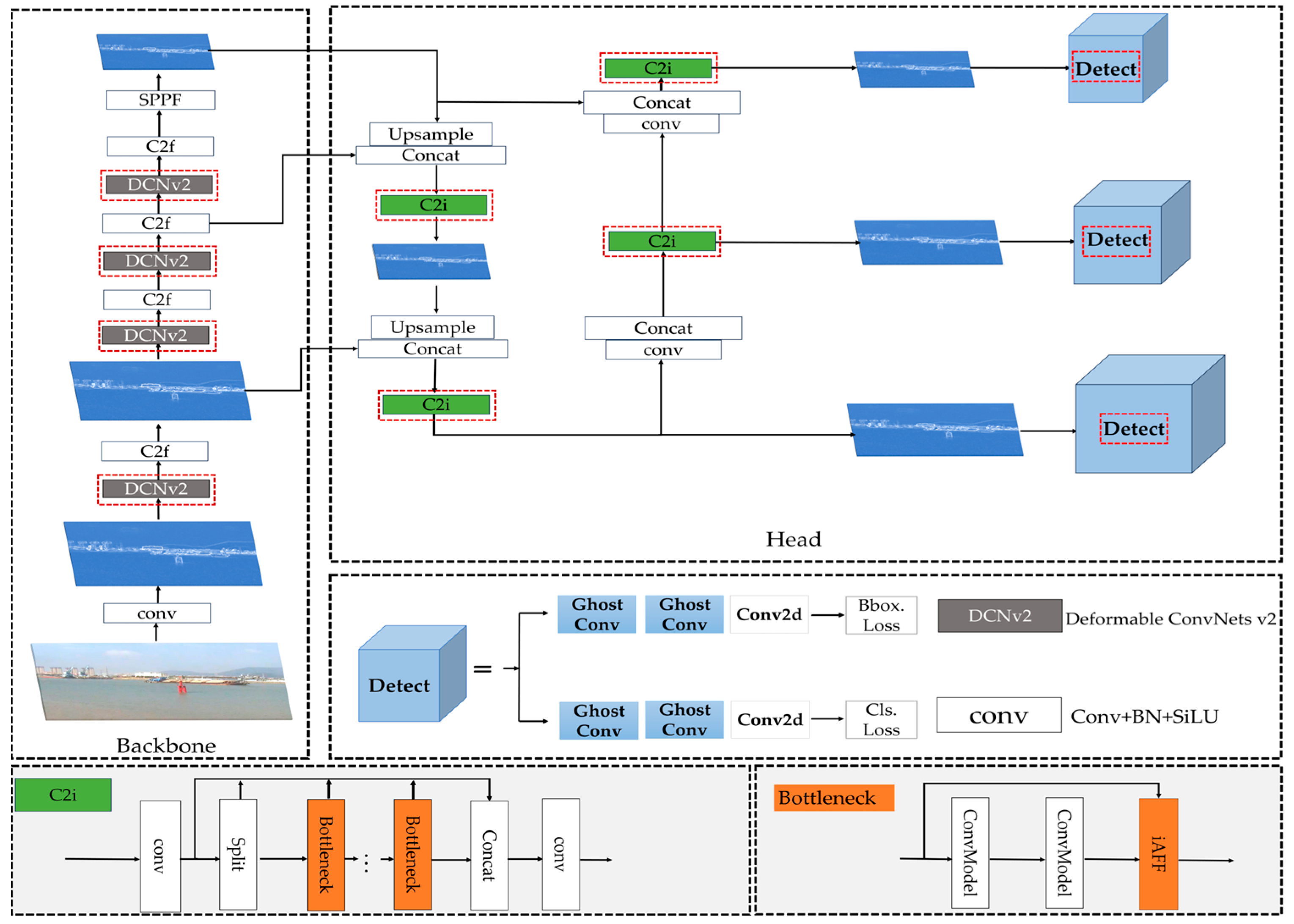
Figure 2. AFF-LightNet model structure diagram. The red box in the figure mainly represents the improved modules of this model. AFF-LightNet mainly consists of two parts. The backbone network is mainly used for feature extraction, while the head network is mainly used for feature fusion and object detection of the features extracted from the backbone network.

Figure 2. AFF-LightNet model structure diagram. The red box in the figure mainly represents the improved modules of this model. AFF-LightNet mainly consists of two parts. The backbone network is mainly used for feature extraction, while the head network is mainly used for feature fusion and object detection of the features extracted from the backbone network.

3.1. DCNv2 Convolution

Although traditional convolution has been widely applied in object detection tasks and has achieved significant success, it can encounter limitations in receptive fields and local connectivity issues when processing large-scale images and complex tasks. These problems stem from the fixed convolution kernel used in traditional convolution, which poses a huge challenge for targets of different scales, rotations, and deformations.

To settle the aforementioned issues, DCN (Deformable Convolutional Networks) [38] was proposed by Zhu Junyan. et al. at the 2017 Computer Vision Conference. It adds offsets on the basis of CNN, which means that in deformable convolution, it is no longer limited to regular networks but is freely sampled on the input feature map according to requirements. The added offset is an additional parameter learned by the network, allowing the convolutional kernel to adapt more flexibly to items with varying scales, rotations, or deformations, consequently advancing the model’s learning ability for complex scenes. DCNv1 [38] is its first version, which enhances CNN’s adaptability to target deformation and position changes in object detection tasks by introducing deformable convolutional layers. It has good effects on feature extraction and enhancing receptive fields. The operation process of it is as follows: first, use a regular grid R with added offset ${\Delta P}_n$ on the input feature map x, and then sum the sampling values weighted by w, which is represented as:

$$R=\left\{\left(-1,-1\right),\left(-1,0\right),\dots ,\left(1,1\right)\right\}$$

(1)

after undergoing deformable convolution, for each position $P_0$ on the output feature map y, it is:

$$y\left(P_0\right)=\sum _{P_n\in R}W\left(P_n\right)\ast \left(P_0+P_n+{\Delta P}_n\right)$$

(2)

among them, $P_n$ represents the nth position, and ${\Delta P}_n$ represents the offset at the nth position.

The sample of DCNv1 activation unit is more inclined to the objects around it, but its target coverage is not comprehensive, and the sample distribution has exceeded the region of interest. To solve these problems, Microsoft Research Asia proposed DCNv2 [39] in 2019, which mainly proposed the Deformable Roll Pooling operation and modulation mechanism. The location is shown as on the output feature map y:

$$y={\sum }_{n=1}^n{W}_n\ast x\left(P+P_n+{\Delta P}_N\right)\ast \Delta M_n$$

(3)

among them, $\Delta M_n$ represents the modulation scalar at the nth position. In order to enhance the sensitivity of deformable convolution to spatial positions, DCNv2 introduces a modulation mechanism, it has the ability to modify both the amplitude and offset of input features at several spatial locations. Under extreme conditions, the module can control the signal that the model does not accept by setting its amplitude to zero, which can reduce the spatial position input response. This modulation mechanism allows the module to freely adjust the spatial support domain for its input data.

3.2. Introducing Iterative Attention Feature Fusion (iAFF)

Attention feature fusion is receiving increasing attention in object detection. AFF is a common method in neural networks that solves the problem of combining features from several tiers by introducing a multi-scale channel attention module (MS-CAM). Its emergence proves the existence of bottleneck problems in initial feature fusion. Based on this, it is proposed to introduce iterative operations into AFF to form iAFF, mainly optimizing the process of feature fusion through iteration.

Simple feature fusion can no longer meet the needs of cross level fusion in object detection. In order to better achieve cross level feature fusion, we propose an improved C2f module, abbreviated as C2i. Figure 3 shows the overall structure of C2i. The original feature fusion is just a simple addition operation, which requires the input feature maps to have the same size and number of channels. Direct addition can lead to information loss and low detection accuracy. However, iAFF can overcome the limitations of addition operations in processing features of different scales, optimize the process of feature fusion through iteration, gradually improve the fusion results, and enhance the performance of the model.

Compared with traditional feature fusion, the features of small ships in images are not obvious and are easily affected by complex backgrounds. Due to the introduction of the MS-CAM module in iAFF, it can integrate features from different scales and semantic inconsistencies, which can better capture the features of small targets. iAFF can also use contextual information to assist in detection. When detecting occluded ships, iAFF can infer the position and information of the occluded part based on the characteristics of the surrounding environment and prior knowledge of the known ships. In addition, the attention weights of iAFF are dynamically adjusted based on input features, and different attention weights are assigned to different input features to highlight important features and suppress irrelevant features, in order to cope with complex and changing detection scenarios.

IAFF as a swift implementation module, can be integrated into any location in the network. Integrate it into the bottleneck of the C2f module in our model. Figure 4 shows the embedding of iAFF at various points within the head network.

3.3. Lightweight Convolution

An essential assurance of the dependability and safety of maritime commerce is ship inspection. Though existing methods are too cumbersome for marine vessel detection and are not suitable for resource limited marine vessel detection equipment. For sorting out this problem, Google first proposed the MobileNet [12] lightweight convolutional network in 2017, and Face++ also raised ShuffleNet [15] in the same year. Moreover, model compression methods include pruning [39], knowledge distillation [40], etc. Although these methods can effectively abate the model’s computational complexity and quantity of arguments, there are still some problems such as high computational density and increased network complexity. Relatively speaking, the GhostNet [17] model can better overcome these problems, mainly using grouped convolution and depthwise separable convolution to reduce model computation and complexity.

In this study, we replaced the ordinary convolution in the head network with GhostConv, aiming to decline the number of model parameters and computational complexity while ensuring that detection accuracy is not affected. It achieves the generation of feature layers through two parts: the main convolution kernel and the auxiliary convolution kernel. The former contains more parameters, while the latter generates more “Ghost” feature maps from the original feature map through low-cost linear transformation. The implementation process is as seen in Figure 5, which includes three main steps: first, the input image is convolved to obtain an intrinsic feature map; then, an operation of linear transformation is performed to generate a Ghost feature map; finally, the intrinsic feature map is concatenated with the obtained Ghost feature map through identity concatenation to obtain the final output. This greatly lessens the computational complexity and parameter count of the model without affecting its performance, making it more suitable for mobile or embedded devices in resource constrained environments.

3.4. Optimizing the Bounding Box Loss Function

The training effect in the object detection task is directly impacted by the loss function selection, convergence speed, and functioning of the model. An excellent bounding box loss function can bring breakthrough performance to the model. However, existing regression loss functions only consider the ratio of intersection and union between the predicted box and the true box, without considering additional geometric factors, which can lead to the problem of gradient vanishing and affect the training effectiveness of the model. SIOU [18] not only considers the overlapping area of bounding boxes but also introduces geometric characteristics such as center point distance, aspect ratio, and angle, which enables SIOU to more accurately describe the differences between predicted boxes and real boxes, thereby improving detection accuracy and robustness.

The SIOU loss function specifically includes four parts: angle cost, distance cost, shape cost, and IOU [34] loss. Angle loss describes the minimum angle between the center point of the predicted box and the true box when connected to the horizontal and vertical distances. The distance loss describes the distance between the predicted box and the center point of the true box, and its penalty cost is proportional to the angle cost; The shape loss mainly considers the aspect ratio between the predicted box and the actual box. It is defined by calculating the difference in width between the two boxes and the maximum width ratio and converges on both sides of the length and width to achieve overall convergence. The definition of the SIOU loss function is:

$${LOSS}_{SIOU}=1-IOU+{\displaystyle \frac{\Delta +\mathsf{\Omega }}{2}}$$

(4)

among them:

$$\Delta =\sum _{t=x,y}\left(1-e^{\gamma \beta t}\right)=2-e^{-\gamma \beta x}-e^{-\gamma \beta y}$$

(5)

$$\mathsf{\Omega }=\sum _{t=w,h}{\left(1-e^{{-w}_t}\right)}^{\theta }={\left(1-e^{{-w}_w}\right)}^{\theta }+{\left(1-e^{{-w}_h}\right)}^{\theta }$$

(6)

where ∆ indicates distance loss, Ω indicates form loss, $P_x$ represents the horizontal distance amid the actual box’s center and the anticipated box’s center, $P_y$ represents the vertical separation between the actual box’s center and the box’s anticipated center, and w represents the weight. The degree of attention to shape loss is controlled by θ, and the range of θ parameter is specified as [2,6].

4. Experimental Results and Analysis

In order to comprehensively verify the effectiveness of our proposed network, we conducted a large number of experiments on the dataset SeaShips7000 [19]. Through qualitative analysis and quantitative evaluation, with different networks, we contrasted the presented network. The following is a detailed explanation of the specific execution process of the experiment and the comparison results.

4.1. Experimental Details

4.1.1. Experimental Environment and Parameter Settings

The experiment of the network model we proposed is based on the Python (1.12.1) software library installed in Ubuntu 22.04, with a programming language of Python 3.9 and an integrated development environment of CUDA 11.8. The CPU model is the 12th generation Intel (R) Core (TM) i5-12490F, running at 3 GHz, and the GPU is NVIDIA GeForce GTX 1080Ti-11G. During the training process, set the learning rate to 0.01, momentum to 0.937, and optimizer weight decay to 0.0005. All input images used in the experiment were adjusted to a pixel size of 640 * 640, the training process epoch was set to 200, the batch size was set to 16, and all other parameters followed the default parameter settings of the YOLOv8 model.

4.1.2. Dataset

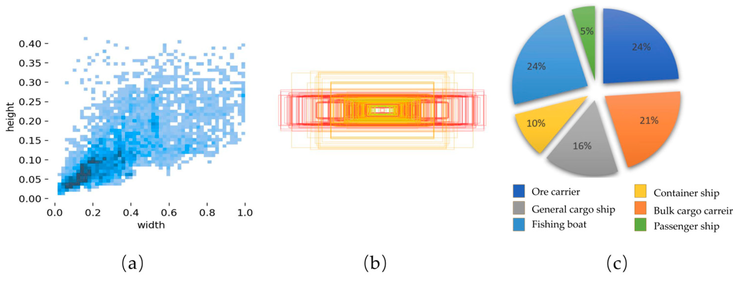
This experiment used the publicly available and free SeaShips7000 dataset, images collected by Wuhan University. It was mainly derived from mobile phones and collation of the monitoring videos of Hengqin Island, Zhuhai, and it comprises six different types of ships, namely: ore ships, bulk carriers, conventional container ships, container ships, fishing ships, and passenger ships. These images have different scales, hull parts, lighting, viewpoints, and occlusion. In this experiment, they were separated into a training set, validation set, and test set in a 3:1:1 ratio. As shown in Figure 6, the figure shows the number of samples contained in each type of ship, the dimensions and corresponding number of bounding boxes in the training set, the distribution of the center point of the bounding box in the image, and the distribution of the target aspect ratio in the training set. 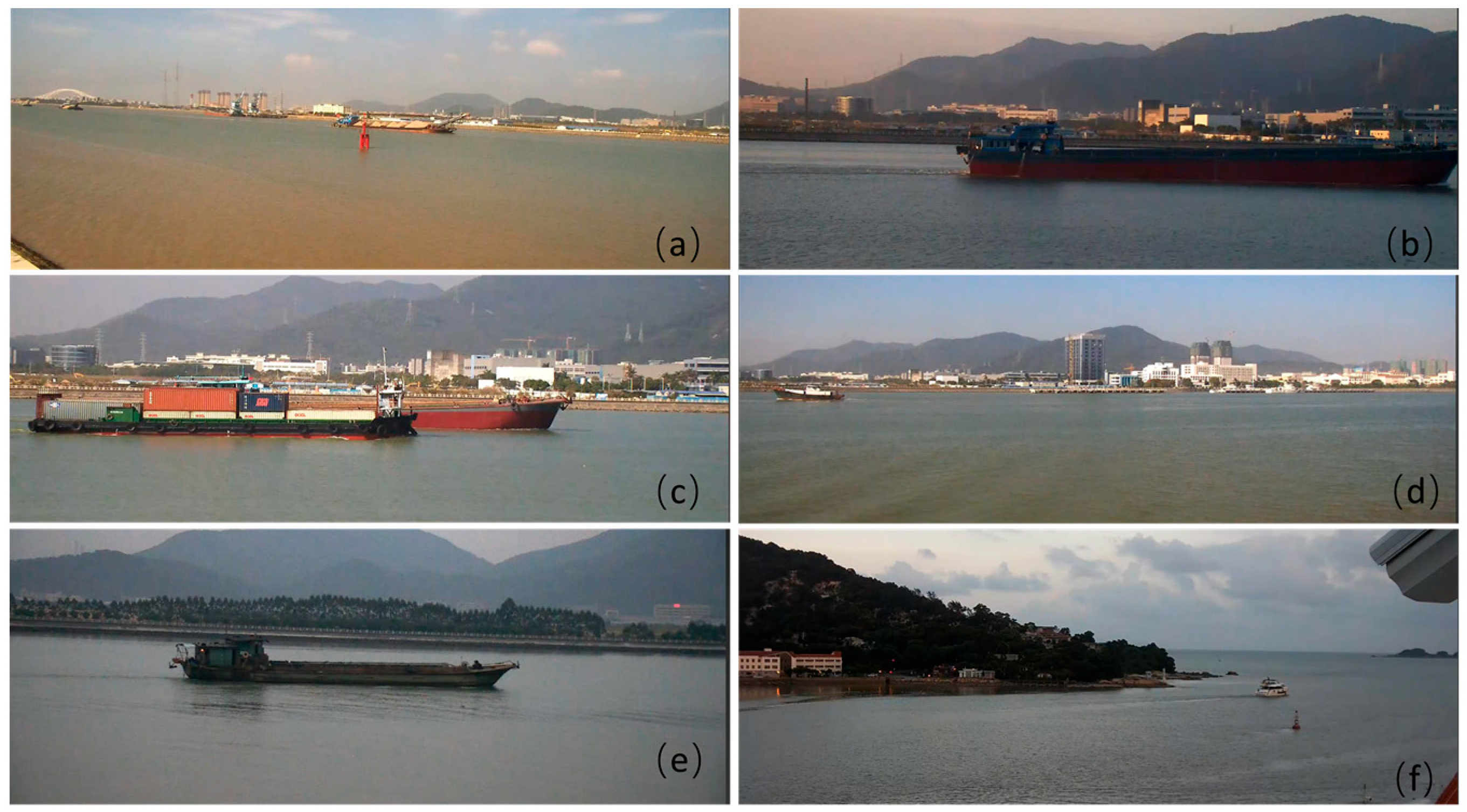Figure 7 shows the six categories of ships in the dataset. The limitations of the offshore filming equipment result in errors in monitoring small targets when monitoring offshore ships, and there is also a certain degree of ambiguity in monitoring distant ships. Ships on the shore are also susceptible to interference from the shore background, which can lead to inadequate monitoring.

4.2. Evaluation Indicators

In our experiments, we primarily employ the objective measurements such as accuracy, recall, F1 score, mAP@0.5, mAP@0.5:0.95, Params, FLOPs, and Traintime to evaluate the availability and efficiency of the proposed model.

Accuracy is the evaluation of the accuracy of a model in object detection tasks, representing the percentage of accurately detected masculine specimen that are truly positive; recall rate is the ability of a model to successfully identify the proportion of positive samples to all true positive samples; the F1 score is the average of accuracy and recall, which comprehensively measures the performance of the model. The larger the F1 score, the better the performance of the model; mAP@0.5 is the average accuracy when the IOU threshold is set to 0.5, which is used to measure the detection accuracy of the model; mAP@0.5:0.95 not only measures the accurateness of the model but also reflects its robustness; Params and FLOPs reflect the model’s quantity of parameters and computational complexity, and the lower they are, the lighter the model is; the training time mainly reflects the efficiency and cost of model training. The shorter the training time, the faster the iteration speed of the model.

4.3. Train Results and Analysis

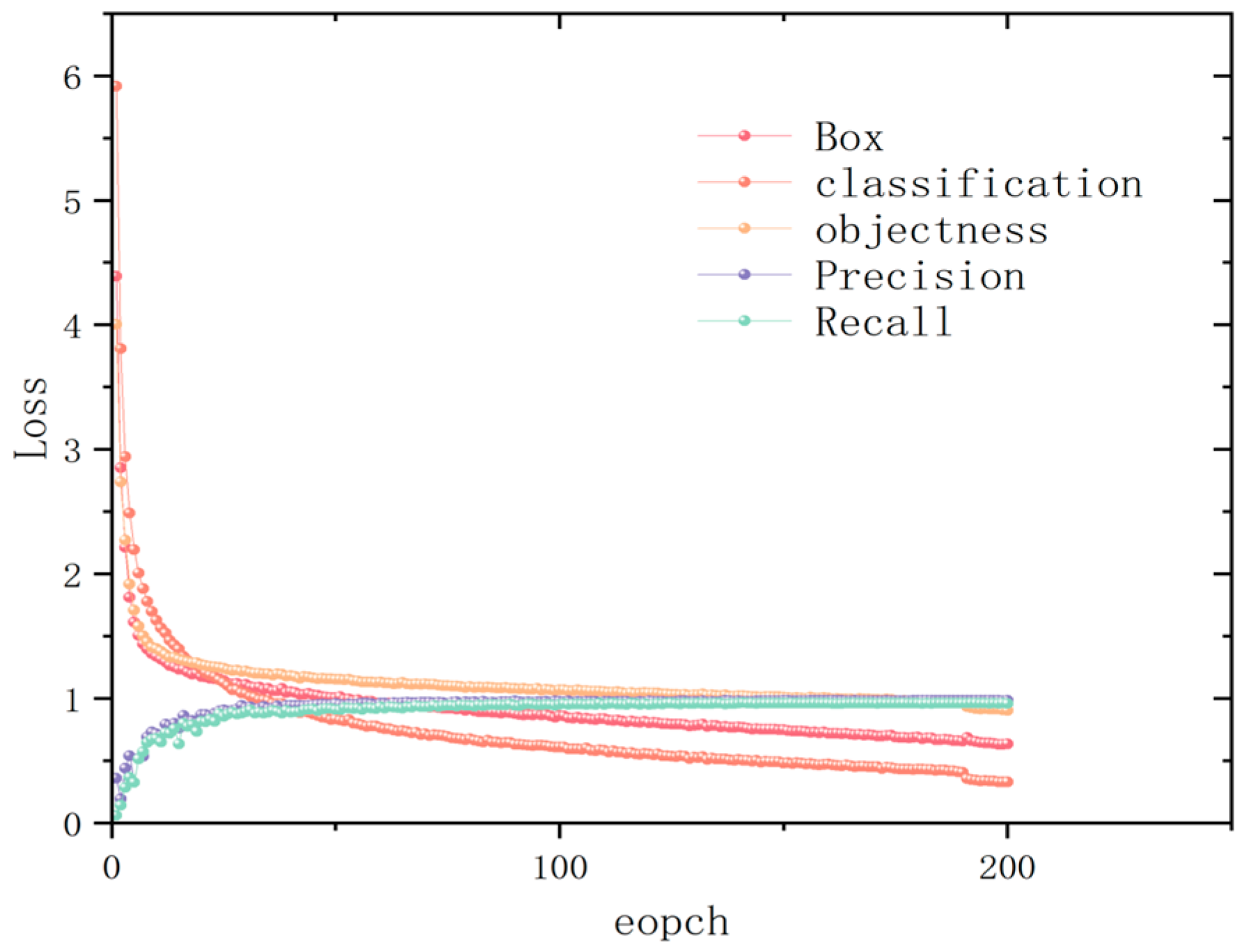
To validate the performance advantage of this method in object detection, we evaluated it on the SeaShips dataset and analyzed its training results. In the experiment, the epoch was set to 200 and the batch size to 16. After 200 rounds of training, the loss curve of AFF-LightNet is shown in Figure 8. From the graph, we can understand that after training, the loss value is continuously decreasing and the convergence speed is also faster, indicating that the model is not overfitting. 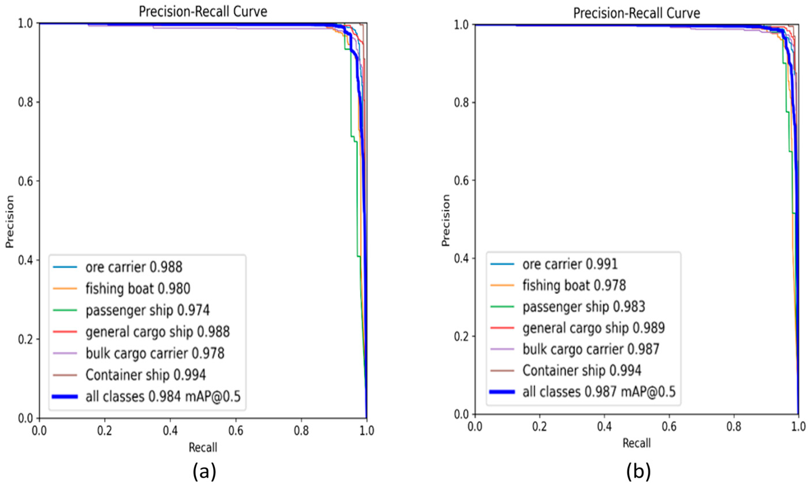Figure 9 shows the P-R (Precision Recall) curve after training. From the graph, we are able to understand that compared with the original YOLOv8 model, our proposed model has an overall mAP better than the original model, indicating that our proposed model has more advantages in performance. Figure 10 shows the F1 score curve. The F1 score curve is a comprehensive indicator of model performance, with higher values indicating better model performance. From Figure 10, we may be aware that our model’s score is higher than that of the original model, which indicates that our model has a better performance advantage compared to the original model.

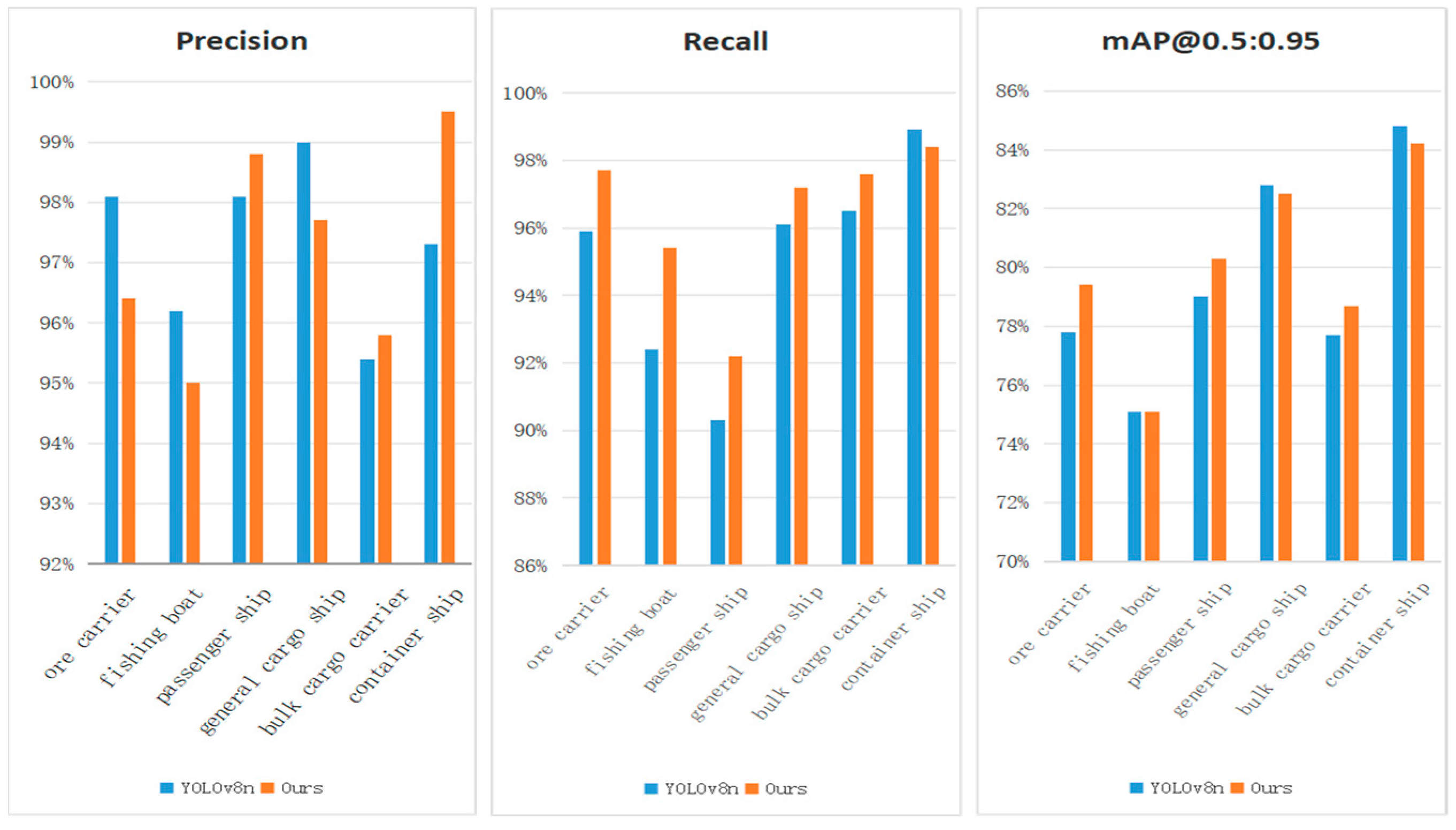
In the bargain, to better demonstrate the detection of different types of ships using our proposed model, we calculated the accuracy, recall, and mAP@0.5:0.95, represented by a bar chart for a more intuitive observation. The experimental outcomes are displayed in Figure 11. We can see that the proposed model has good detection performance for bulk cargo ships, container ships, and passenger ships, but its detection accuracy for fishing boats, mineral sand ships, and general cargo ships is lower than YOLOv8n. This is because the loss function SIOU introduced by the proposed model is more conducive to the localization and regression of large targets, and inappropriate adjustment of category weights affect the detection of small targets. In addition, the introduced variability convolution increases the model’s receptive field, which can lead to a decrease in detection accuracy for some targets if the receptive field is too large.

4.4. Qualitative Evaluation

In an effort to better evaluate the performance of our proposed model, in this section we will evaluate our model from a visual perspective. Firstly, we visually compare our model with the original model, and the outcomes are displayed in Figure 12. It displays the comparison outcomes between our model and the original model under different lighting conditions. The first column is the unprocessed image, the second column is the detection result of the original model, and the third column is the detection result of the newly proposed model. The three images were taken in the morning, noon, and evening, respectively. The proposed model introduces a module with attention mechanism, which dynamically assigns weights based on the input image, making the model more focused on task-related information, reducing the interference of redundant information and, thus, improving detection accuracy. From the figure, we can see that our model has higher accuracy in ship detection than the original model under weak and strong light conditions. In addition, we will visually compare our model with other models for different scale targets (small, medium, and large targets). The experimental results are shown in Figure 13. It can be observed that the features extracted by our model are relatively inadequate for the detection of large targets, due to their long distance and low resolution, so the detection accuracy of the proposed model is the second best. By contrast, the comparative models have the best results, as they provide adequate features and can learn more information. Moreover, the detection of small targets is the most challenging, as they have fewer discriminative features, resulting in the lowest detection accuracy. The proposed model also presents similar challenges, but it has the best detection accuracy for different scales.

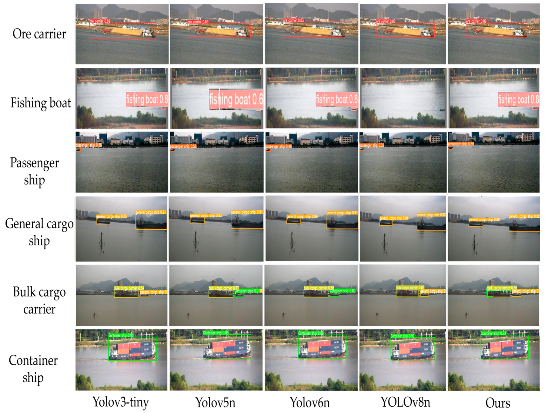
Finally, we also visually compared our model with other models under different types of ships, and the experimental results are shown in Figure 14. Due to the large overlap area when multiple ships appear simultaneously, obstructed ships are difficult to identify and locate, making it difficult for ships to be detected, resulting in unreliable maritime traffic monitoring. We can see that when multiple ships appear simultaneously, YOLOv5 and YOLOv6 experience missed or false detections. They are unable to distinguish the obstructed container ships and also detect the general cargo ships as container ships. For the detection of small targets, YOLOv8 cannot detect fishing boats since the features of small targets may be interfered with by other target information during the fusion process, which makes it difficult for the model to recognize their features. However, iAFF embedded in the MS-CAM module can integrate features from different scales, so it performs well in feature fusion. The angle loss introduced by SIOU finds the direction of the bounding box from different directions, making the model more accurate in detecting occluded and small targets.

4.5. Quantitative Evaluation

In order to evaluate the performance of the AFF-LightNet model from multiple perspectives, this section will compare it quantitatively. We conducted quantitative evaluations on other YOLO series. The YOLO series includes YOLOv3-tiny, YOLOv5n, YOLOv6n, and YOLOV8. The experimental results are shown in Figure 15 and

Table 1. Comparison of different algorithms within SeaShips dataset.

Methods	Precision (%)	Recall (%)	${\mathit{F}}_1$ Score (%)	mAP@0.5 (%)	mAP@0.5:0.95 (%)	Params (M)	FLOPs (G)
YOLOv3-tiny	97.2	94.4	95.78	98.0	78.0	12.12	18.9
YOLOv5n	97.4	95.4	96.40	98.2	78.1	2.50	7.1
YOLOv6n	97.5	95.3	96.40	97.8	79.1	4.23	11.8
YOLOv8n	97.3	95.8	96.54	98.4	79.4	3.00	8.1
Ours	97.6	95.5	96.54	98.8	80.2	2.81	6.2

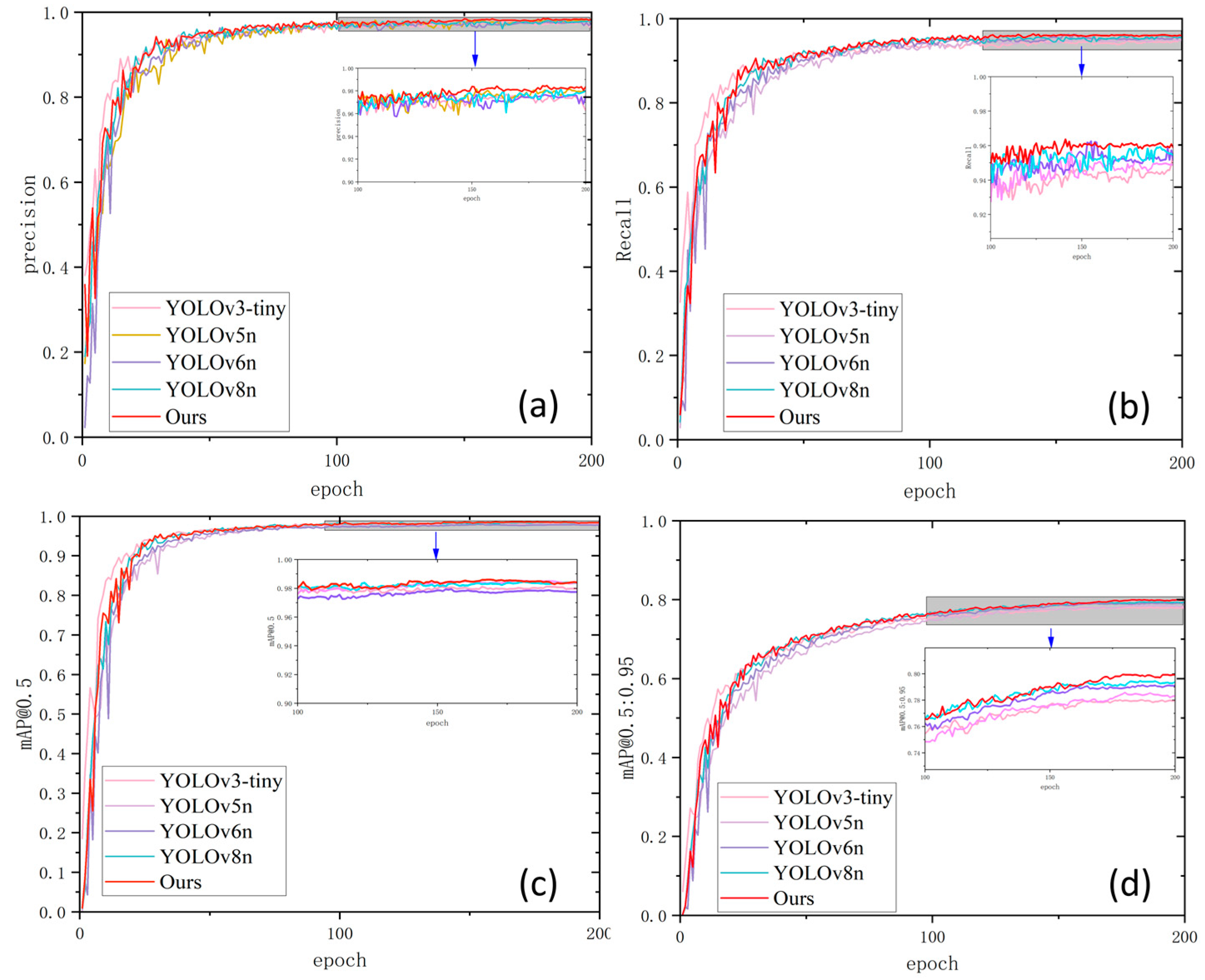
. Figure 15 shows the accuracy, recall, mAP@0.5, and mAP@0.5:0.95 within 200 model training cycles; it is 0.95. The figure shows that as the number of training iterations increases, the parameters of the model are better optimized, and more features can be learned. The feature extraction ability is constantly improving. Meanwhile, the addition of lightweight and attention mechanism modules in the model reduces the computational resources and improves detection accuracy. As a result, the model gradually learns how to generalize to unknown data with the increase in epochs. Thus, our model performs better than other competitors, with a slow curve rise and fast convergence speed, indicating that our model does not overfit. From Table 1, it can be seen that the YOLOv5n model uses MobileNetV3 and anchor-free detection methods, significantly reducing its parameter count, but its detection accuracy is not as good as other comparative YOLO models. The proposed model leverages lightweight modules and feature fusion modules, which can better capture significant features in the image while reducing computational resources. Therefore, our model performs the best.

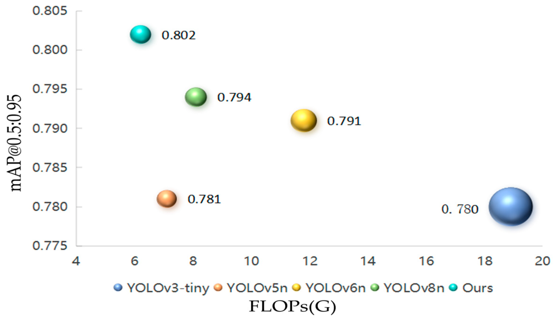
Figure 16 shows the performance of AFF-LightNet and other models in terms of FLOP, parameter count, and mAP@0.5 as well as mAP@0.5:0.95. The size of each ball area represents the sum of parameters. As shown in the figure, our model achieves higher detection accuracy with fewer parameters and lower complexity. Compared with other models, the model proposed in this paper achieves a better balance between model size and detection accuracy.

Table 1 shows the comparison between our model and the YOLO series models. As can be observed from the data, our model achieved the best performance among them due to its accuracy, F1 score, mAP@0.5, and mAP@0.5:0.95, which are the highest, and although our model is not the lightest, it is also in second place. The lightest size is 2.50 MB, while our model size is 2.81 MB. To verify that our network is more lightweight, we compared our model with other lightweight networks, currently popular lightweight networks that include MobileNetV3 and ShuffleNetV2. The experimental results are shown in

Table 2. Comparing the performance of distinct lightweight modules on SeaShips dataset.

Methods	Precision (%)	Recall (%)	${\mathit{F}}_1$ Score (%)	mAP@0.5 (%)	mAP@0.5:0.95 (%)	FLOPs (G)	Params (M)	FPS
MobileNetV3	97.6	96.3	97.0	98.5	80.8	9.4	5.65	285.7
ShuffleNetV2	97.0	96.0	96.5	98.2	78.8	7.4	2.79	434.8
GhostConv	97.5	96.5	97.1	98.3	79.9	6.7	2.64	625.0

. The chart indicates that although our network’s detection accuracy is not the best, its computational complexity and parameter quantity are both optimal, achieving the desired detection effect. Furthermore, the test velocity of the presented network model reaches a high standard among similar detection models, which demonstrates the powerful ability of our network to achieve real-time and latency-free detection, that is, to achieve real-time detection.

Furthermore, we also compared our model with some models from recent years, and the comparison results are shown in

Table 3. Comparison of our model with other models on the SeaShips dataset.

Methods	Precision (%)	Recall (%)	${\mathit{F}}_1$ Score (%)	mAP@0.5 (%)	mAP@0.5:0.95 (%)	Params (M)	FLOPs (G)
MC-YOLOv5s [41]	96.3	93.1	95.0	97.5	-	6.74	5.8
YOLOv7-RCBAM [42]	95.6	89.3	92.3	96.1	-	-	-
Improve YOLOX [43]	96.3	96.2	96.2	98.2	-	-	-
LSDNet [44]	97.9	96.6	97.2	98.5	76.0	6.02	13.1
Ours	97.6	95.5	96.5	98.8	80.2	2.81	6.2

. From the table, our model does better than other models in terms of mAP@0.5, mAP@0.5:0.95, and parameter quantity. Although its computational complexity is not the lowest, it is among the lowest.

4.6. Ablation Experiment

To validate the effectiveness and efficiency of the proposed model, we conducted a sequence of ablation tests on the components of the AFF-LightNet model (on the SeaShips dataset). The architecture and experimental details of AFF-LightNet are shown in

Table 4. Comparing the effectiveness of distinct modules for ship detection.

Number	iAFF	GhostConv	DCNv2	SIOU	Params (M)	FLOPs (G)	mAP@0.5 (%)	mAP@0.5:0.95 (%)
N1					3.00	8.1	98.4	79.9
N2	✓				3.11	8.1	98.2	80.1
N3	✓	✓			2.75	6.7	98.8	80.1
N4	✓		✓		3.17	7.6	98.3	79.6
N5	✓	✓	✓		2.86	6.3	98.4	80.2
N6	✓	✓	✓	✓	2.81	6.2	98.8	80.2

(√ indicates the introduction of improved modules). The visual representation reveals that when adding iAFF, although its parameter counts increase, mAP@0.5:0.95 significantly increased. When GhostConv and iAFF were added, their number of parameters and computational complexity were significantly reduced, but their accuracy was still not high enough. Therefore, DCNv2 and SIOU were added, and the results clearly showed that their computational complexity and detection accuracy improved after addition.

It is obviously visible from Table 4 that the proposed AFF-LightNet attains both lightweight and more elevated detection accuracy than the original model, indicating that our proposed AFF-LightNet model achieves a better balance between lightweight and improved accuracy. On top of that, we also conducted ablation experiments on the effects of various components of the AFF-LightNet model architecture on various types of ships. The specific experimental results are shown in

Table 5. Comparison of detection performance of different modules for various types of ship.

Methods	mAP@ 0.5(%)						mAP@ 0.5:0.95 (%)	Precision (%)	Recall (%)	F1 Score (%)	FLOPs (G)
	Ore Carrier	Fishing Boat	Passenger Ship	General Cargo Ship	Bulk Cargo Carrier	Container Ship
Yolov8n	98.8	97.6	96.3	99.0	98.8	99.4	79.7	97.3	95.5	96.40	8.1
+iAFF	99.0	97.5	97.1	98.5	98.1	99.5	80.1	97.7	95.5	96.58	8.1
+GhostConv	98.8	97.4	97.0	99.1	98.3	99.5	79.9	97.5	96.5	96.71	6.7
+DCNv2	99.2	97.4	97.8	99.3	99.0	99.5	80.3	97.2	96.4	96.80	7.5
+SIOU	98.6	97.7	96.7	99.3	97.9	99.4	80.0	98.0	95.1	96.53	8.1

. It is observable in the table that compared with the original YOLOv8n, the introduction of iAFF and DCNv2 can significantly improve detection accuracy, while the loss function can improve detection accuracy. Although GhostConv does not significantly improve detection accuracy, it greatly reduces computational complexity.

To verify the reliability of the proposed method, we compared the detection of different feature fusion modules in the model, and the results are shown in

Table 6. Performance comparison of different feature fusion modules on the SeaShips dataset.

Methods	Precision (%)	Recall (%)	${\mathit{F}}_1$ Score (%)	mAP@0.5 (%)	mAP@0.5:0.95 (%)	FLOPs (G)	Params (M)	Traintime (h)
Baseline	97.5	95.7	96.70	98.4	79.9	8.1	3.00	2.24
+Bifpn	96.9	95.7	96.30	98.5	80.0	8.1	3.00	2.26
+slimneck	97.9	95.6	96.73	98.4	80.0	7.4	2.79	2.34
+iAFF	97.7	95.5	96.61	98.5	80.1	8.1	3.11	2.22

. From the table, it can be seen that when our model is mAP@0.5 and mAP@0.5:0.95, it performs the best. Although it has a higher number of parameters than other modules, our training time is the least and our top inference speed illustrates how well our model number of iAFFs added is also one of the factors affecting the accuracy of the hard model. In this model, we introduced different numbers of iAFFs into C2f, and the experimental results are shown in

Table 7. Comparison of C2i results at different positions.

Methods	Precision (%)	Recall (%)	${\mathit{F}}_1$ Score (%)	mAP@0.5 (%)	mAP@0.5:0.95 (%)	Params (M)
a	98.1	95.3	96.7	98.3	80.0	3.0
b	97.0	95.9	96.4	98.2	80.0	3.0
c	96.1	96.6	96.3	98.5	79.9	3.0
d	97.7	95.5	96.6	98.5	80.1	3.1

. The experimental results show that introducing iAFF into each C2f module in the head network has the best effect. As the number of iAFFs increases, the model can further explore and utilize the correlation and complementarity between these characteristics, hence increasing feature fusion’s efficacy; through an iterative attention mechanism, the model can gradually emphasize on the crucial specifics of the entering image, ignore irrelevant information and, thus, ameliorate the sensitivity and accuracy of the model to target features. To verify the good performance of the loss function SIOU on our model, we conducted experiments on the SeaShips dataset, and the experimental results are shown in

Table 8. Performance comparison of different loss functions within SeaShips dataset.

Methods	Precision (%)	Recall (%)	${\mathit{F}}_1$ Score (%)	mAP@0.5 (%)	mAP@0.5:0.95 (%)
CIOU	97.7	96.6	97.15	98.7	83.8
WIOU	97.6	97.5	97.55	99.0	83.8
EIOU	98.7	96.6	97.63	99.1	83.9
SIOU	98.2	97.0	97.60	99.1	84.0

. From the table, we can see that SIOU provides a more comprehensive and accurate loss metric by considering more geometric characteristics of bounding boxes, thereby helping the model optimize bounding box prediction better during training. Compared to other loss functions, SIOU performs better in this model.

5. Conclusions

In this paper, a lightweight network architecture is presented for efficient detection of ships in ocean monitoring systems, bringing improved technological solutions to the field of ocean monitoring. The proposed model introduces iAFF and GhostConv based on YOLOv8n, ensuring detection accuracy while achieving lightweight, making it more suitable. For resource-limited offshore mobile improvement of the model’s target localization and robustness, we substituted CIOU with SIOU, which helps the model converge more stably during the training process. Finally, we conducted extensive experiments on the dataset SeaShips7000, and the experimental results showed that the model has good performance in both lightweight and detection accuracy. Compared with other ship detection methods, our method not only demonstrates high efficiency in computational complexity but also achieves satisfactory levels of detection accuracy. However, faulty sensors can still result in significant differences or missing data in the collected data, thereby affecting the measurement of differences between the actual box and the predicted box. Different noises can lead to incorrect gradient information, affecting the adjustment of model parameters, resulting in a decrease in training rate and, thus, limiting the performance of the model. Looking ahead, in order to further enhance the overall performance of this method, we can explore and optimize it in the following directions:

• The dataset used in the proposed model consists entirely of static ship images, and the model is too simplistic. Therefore, in future research, our goal is to incorporate videos into the model, while maintaining a balance between lightweighting and detection accuracy.
• Maritime monitoring systems take photos from a two-dimensional perspective. When ships are obstructed or overlapping, it can lead to missed or false detections. Therefore, optical images can be combined with remote sensing images to effectively avoid missed or false detections and improve the performance of the model.