Application of Computational Fluid Dynamics and Semi-Empirical Speed Loss Prediction for Weather Routing

Abstract

This study presents an optimized system for ship route planning. Computational fluid dynamics simulations were used to modify Kwon’s semi-empirical speed loss estimation method, enabling efficient route planning under variable sea conditions. The study focused on improving the prediction of speed loss in irregular waves for container ships and further applying this to ship-optimized voyage planning. Dynamic programming was used for optimized voyage planning by modifying the ship course in response to meteorological data; this approach could balance both energy efficiency and safety. The modified speed loss predictions aligned closely with the simulation results, enhancing the reliability of weather routing decisions. Case studies for trans-Pacific and trans-Atlantic voyages demonstrated that the proposed system could significantly reduce the voyage time. These findings highlight the potential of real-time updates in voyage planning. The proposed system is a valuable tool for captains and fleet managers. The applicability of this system can be further broadened by validating it on different ship types.

1. Introduction

Ship operators are required to meet many new regulatory statutes and market needs. This requirement has stimulated the development of weather routing systems and voyage optimization methods for shipping routes in ocean-crossing voyages. This paper presents a weather routing system based on dynamic programming that provides an optimal route with respect to voyage time, fuel consumption, and cargo or hull damage. The proposed system emphasizes both safety and route planning, which are critical for navigation and rely on precise oceanographic and meteorological data.

Owing to advancements in weather forecast data collection methods, maritime operators can now obtain up-to-date synoptic and forecast charts by simply turning a dial. However, correctly interpreting these charts to forecast the vessel’s performance under a present set of weather conditions is still challenging. The proposed voyage optimization system is fast when updating ship routes in real time. Real-time route updates enable captains and fleet managers to safely and effectively plan the course and speed of the ship between a given pair of departure and destination ports. The proposed system considers not only the weather conditions for any given voyage but also the ship’s performance.

The commonly used routing algorithms for minimizing fuel consumption or voyage time are based on the calculus of variations, the isochrone method, the isopone method, and two-dimensional (2D) dynamic programming. The calculus of variations [1] is about finding a stationary function that maximizes or minimizes some functional (most commonly of arc length). Optimization is achieved by varying the parameters that control a given trajectory, such as time or velocity. The isochrone method [2] is a practical deterministic approach for calculating the minimum-time route; optimization is achieved by varying the ship’s course while assuming constant engine power. The isopone method [3] involves determining the optimal track by defining planes of equal fuel consumption (energy fronts) instead of time fronts.

A modified isochrone method has also been developed [4], wherein a three-dimensional (3D) model is used. The modified method considers the variation in sea conditions during voyages and ensures that land is avoided. The iterative dynamic programming algorithm for optimized voyage planning is another algorithm designed to solve routing problems [5]; however, this algorithm is computationally complex, requires long simulation times, and cannot use up-to-date ship conditions. Other relevant algorithms include the augmented Lagrange multiplier [6], the Dijkstra algorithm [7,8,9], which has established weight functions based on the weather forecast at sea and the reduction in ship speed, and the genetic algorithm [10].

2D dynamic programming is an optimization approach grounded in Bellman’s principle of optimality, offering similarities to the modified isochrone method. This technique allows operators to define navigation boundaries in maritime applications by utilizing a suitable grid system. Wei and Zhou [11] introduced a new forward 3D dynamic programming method derived from 2D dynamic programming aimed at optimizing fuel consumption during voyages. Their approach achieves fuel efficiency by accounting for variations in a vessel’s course and speed over time across diverse geographic locations.

Calculating speed loss is crucial for evaluating a ship’s performance in open-sea conditions and assessing its environmental impact. Several researchers have explored the calculation of speed loss in a seaway. Journée [12,13] applied and experimentally validated an approximation method to study the effects of ship motion on propeller performance. Faltinsen [14] investigated resistance and propulsion in seaways and asserted that because the frequency of encounters with incoming waves is considerably lower than the propeller rotational frequency, only vertical velocity due to ship motion substantially affects propeller performance in waves. Furthermore, Nakatake et al. [15] developed a panel method using source and sink distributions to simulate the ship hull, propeller, and rudder. They computationally investigated the interactions among these three components. Kashiwagi et al. [16] investigated propeller performance in waves using the enhanced unified theory, which is derived from ship motion theory. Martic et al. [17] evaluated the added resistance in waves using the 3D panel method based on the Kelvin-type Green function. Lastly, Chuang and Steen [18] conducted experiments to analyze ship power and speed loss in waves. Jasna and Odd [19] provided empirical evidence for the claim that speed loss is influenced more by changes in the sea state than by the added resistance experienced by a ship in waves. Chuang and Sverre [20] performed model tests to predict the thrust deduction factor in waves; the results demonstrated that the heading angle to the beam sea played a greater role than added wave resistance.

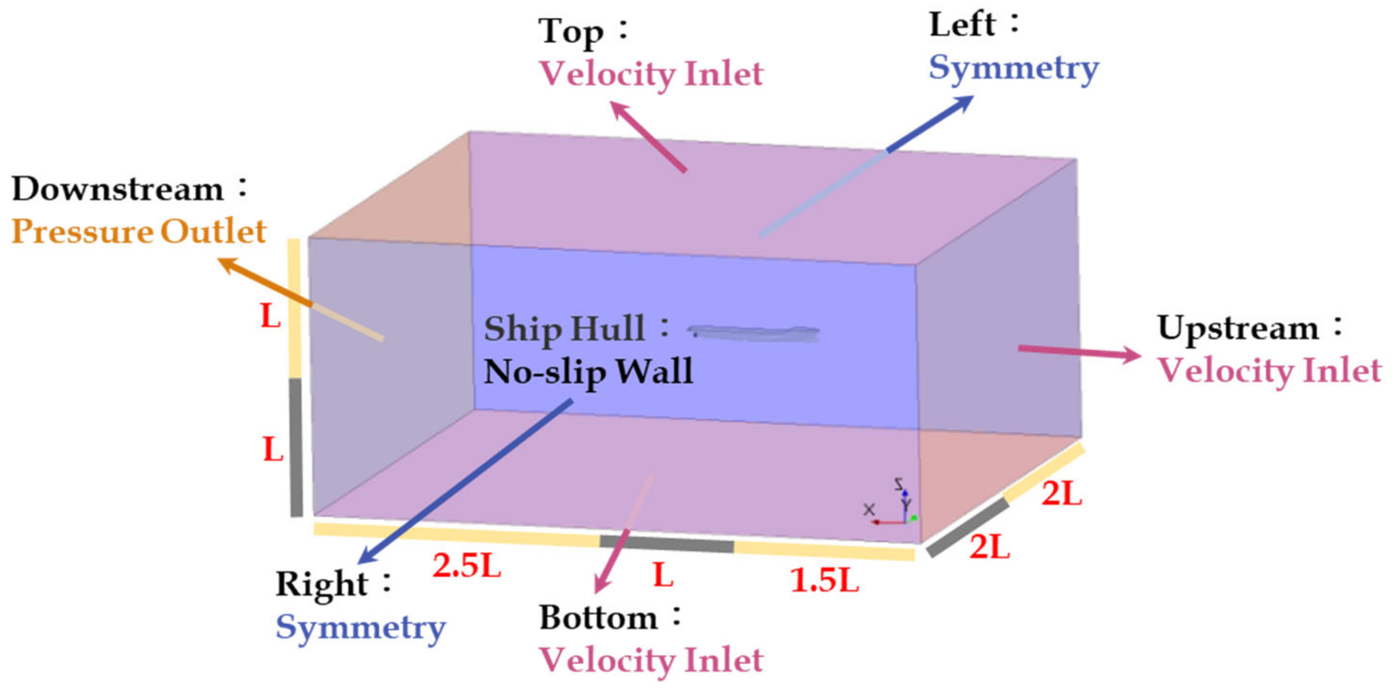
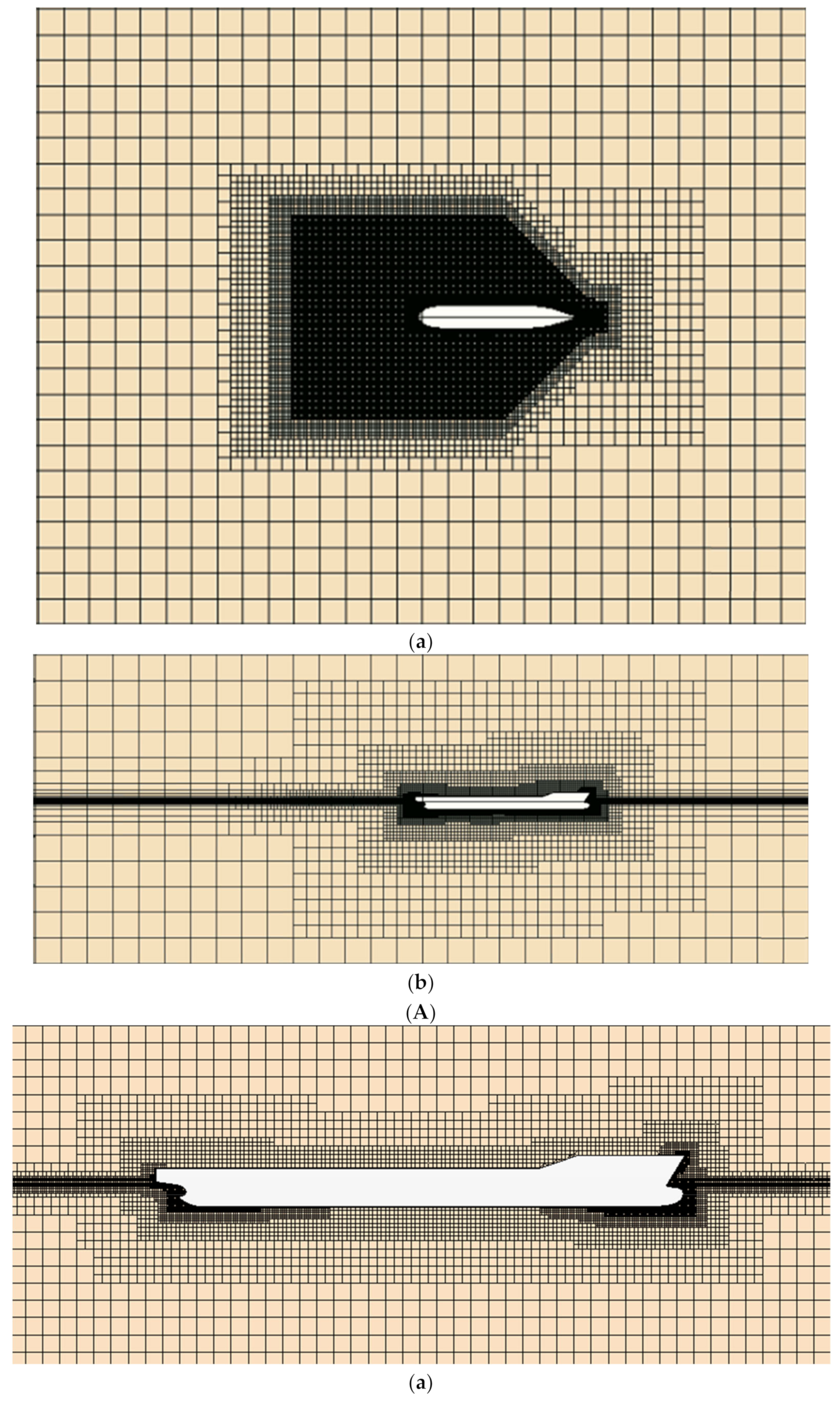
Computational fluid dynamics (CFD) techniques are a widely recognized and robust method for evaluating the speed loss of ships through self-propulsion simulations under various ship design scenarios. Dai et al. [21] used CFD with a Reynolds-averaged Navier–Stokes (RANS) approach to compute propeller open water simulations and self-propulsion simulations in calm water and head and oblique waves. Kim et al. [22] applied CFD with an Unsteady RANS approach to calculate the added resistance and ship motion in waves with different headings. Hsin et al. [23], Lin et al. [24], and Lu et al. [25] have computed speed loss through simulated self-propulsion tests in calm water and in waves. The aforementioned studies applied different approaches for conducting self-propulsion tests. Moreover, full-scale CFD self-propulsion simulations employing RANS were conducted by Mikulec and Piehl [26] and Saydam et al. [27], whose findings were validated through sea trials involving a 555.75-ton displacement research vessel and a 9060-ton displacement tanker, respectively. Similarly, Farkas et al. [28] conducted full-scale CFD simulations of hull resistance, propeller open water, and self-propulsion tests to estimate the benefits of speed reduction strategies, such as slow steaming, in realistic sailing conditions.

Furthermore, the Marine Environment Protection Committee (MEPC) within the International Maritime Organization [29] and Kwon [30] have developed empirical formulae that efficiently estimate speed loss. These formulae are based on the assumption of constant engine performance, thereby obviating the need for complex measurements of added resistance, propulsion factors, or propeller characteristics.

The subsequent section reviews existing speed loss estimation methods and introduces a modification to Kwon’s equation proposed in the present study.

2. Estimation of Speed Loss in Ships

This section discusses Kwon’s method and the empirical formula proposed by the MEPC. It also presents the results of CFD simulations and a novel modification to Kwon’s formula, introduced to better approximate the speed loss of a ship using the proposed weather routing system.

2.1. Model Ships

The KRISO Container Ship (KCS) [31,32], designed by the Korea Research Institute of Ships and Ocean Engineering (KRISO), served as the reference for all calculations of speed loss in ships. The KCS is a modern container ship that features a well-defined hull with a bulbous bow and stern, making it a widely recognized benchmark model for the study and validation of CFD methods. The main parameters of the KCS are presented in

Table 1. Main parameters of the KCS.

	Full Scale	Model Scale
Scale factor, $\lambda$	1	31.599
Length between perpendiculars, $L_{PP}$ (m)	230.0	7.279
Length of waterline, $L_{WL}$ (m)	232.5	7.358
Breadth, $B$ (m)	32.2	1.019
Depth, $D$ (m)	19.0	0.601
Draught, $T$ (m)	10.8	0.342
Displacement volume, ∇ (m3)	52,030	1.649
Wetted surface area w/o rudder, $S$ (m2)	9530	9.544
Block coefficient, $C_B$	0.651	0.651
Midship section coefficient, $C_M$	0.985	0.985
Longitudinal center of buoyancy, $LCB$ (%), fwd+	−1.48	−1.48
Longitudinal center of gravity, $LCG$ (m)	111.6	3.532
Vertical center of gravity, $VCG$ (m)	7.28	0.182
Metacentric height, $GM$ (m)	0.60	0.019
Ratio between roll radius of gyration and breadth, $K_{xx}/B$	0.40	0.40
Ratio between pitch radius of gyration and length, $K_{yy}/L_{PP}$	0.25	0.25
Service speed at 85% MCR, $V_{knot}$ (knots)	24.0	4.069
Service speed at 85% MCR, $V$ (m/s)	12.35	2.197

Moment of inertia: $I_{xx}={K_{xx}}^2\times mass$. $I_{yy}={K_{yy}}^2\times mass.$

, and a model of the ship, with a scale ratio of 1:31.599, is illustrated in Figure 1. CFD simulations were conducted to analyze wave-added resistance and ship motion in regular wave conditions.

2.2. Semi-Empirical Formula: Kwon’s Method

Kwon’s method [30] extends existing weather formulae and incorporates insights from various researchers’ calculations of speed loss by wind, motion, and wave-added resistance. This method predicts speed loss in irregular wave and wind conditions and is applicable across a broad range of scenarios, with block coefficients ranging from 0.55 to 0.85 and Froude numbers from 0.05 to 0.30. According to Kwon, the predictions align closely with experimental towing tank data, demonstrating the method’s reliability.

According to Kwon’s method, the percentage of speed loss can be calculated using Equation (1).

$${\displaystyle \frac{\Delta V}{V_1}}=C_{\mu }\cdot \Delta R\cdot C_F$$

(1)

The speed loss is calculated as follows: $\Delta V=V_1-V_2$, where $V_1$ denotes the design speed in calm seas (i.e., no wind or waves), and $V_2$ denotes the ship speed in selected wind and wave conditions. The design speed $V_1$ can be obtained from Equation (2).

$$V_1=Fr\cdot \sqrt{L_{PP}\cdot g}$$

(2)

where $Fr$ denotes the ship’s Froude number, $L_{PP}$ denotes the ship length between perpendiculars, and $g$ denotes acceleration due to gravity. All units are expressed in SI units.

The speed loss calculation also requires the weather direction reduction coefficient $C_{\mu }$, the speed correction factor $\Delta R$, the ship form coefficient $C_F$, and the Beaufort scale $BN$ [33]. These parameters are listed in

Table 2. Weather direction reduction coefficient $C_{\mu }$.

Weather Direction	Direction Angle (to the Ship’s Bow) $\mathit{\beta }$	Direction Reduction Coefficient ${\mathit{C}}_{\mathit{\mu }}$
Head sea (irregular waves) and wind	0°	$2C_{\mu }=2$
Bow sea (irregular waves) and wind	30° to 60°	$2C_{\mu }=1.7-0.03(BN-4{)}^2$
Beam sea (irregular waves) and wind	60° to 150°	$2C_{\mu }=0.9-0.06(BN-6{)}^2$
Following sea (irregular waves) and wind	150° to 180°	$2C_{\mu }=0.4-0.03(BN-8{)}^2$

,

Table 3. Correction factor $\Delta R$.

$\mathbf{Block} \mathbf{Coefficient} {\mathit{C}}_{\mathit{B}}$	Ship Loading Conditions	$\mathbf{Speed} \mathbf{Correction} \mathbf{Factor} \mathsf{\Delta }\mathit{R}$
0.55	Normal	$1.7-1.4Fr-7.4(Fr{)}^2$
0.60	Normal	$2.2-2.5Fr-9.7(Fr{)}^2$
0.65	Normal	$2.6-3.7Fr-11.6(Fr{)}^2$
0.70	Normal	$3.1-5.3Fr-12.4(Fr{)}^2$
0.75	Loaded or normal	$2.4-10.6Fr-9.5(Fr{)}^2$
0.80	Loaded or normal	$2.6-13.1Fr-15.1(Fr{)}^2$
0.85	Loaded or normal	$3.1-18.7Fr-28.0(Fr{)}^2$
0.75	Ballast	$2.6-12.5Fr-13.5(Fr{)}^2$
0.80	Ballast	$3.0-16.3Fr-21.6(Fr{)}^2$
0.85	Ballast	$3.4-20.9Fr-31.8(Fr{)}^2$

,

Table 4. Ship form coefficient $C_F$.

Type of (Displacement) Ship	$\mathbf{Ship} \mathbf{Form} \mathbf{Coefficient} {\mathit{C}}_{\mathit{F}}$
All ships (except container ships) in loaded loading conditions	$0.5BN+{BN}^{6.5}/({2.7\nabla }^{{\displaystyle \frac{2}{3}}})$
All ships (except container ships) in ballast loading conditions	$0.7BN+{BN}^{6.5}/({2.7\nabla }^{{\displaystyle \frac{2}{3}}})$
Container ships in normal loading conditions	$0.7BN+{BN}^{6.5}/({22.0\nabla }^{{\displaystyle \frac{2}{3}}})$

,

Table 5. Beaufort scale and corresponding wind speeds.

$\mathit{B}\mathit{N}$	Wind Description	$\mathbf{Wind} \mathbf{Speed} (\mathbf{m}/\mathbf{s})$
0	No wind	<0.3
1	Gentle current of air	0.3–1.5
2	Gentle breeze	1.5–3.3
3	Light breeze	3.3–5.5
4	Moderate breeze	5.5–8.0
5	Fresh breeze	8.0–10.8
6	Strong wind	10.8–13.9
7	Stiff wind	13.9–17.2
8	Violent wind	17.2–20.7
9	Storm	20.7–24.5
10	Violent storm	24.5–28.4
11	Hurricane-like storm	28.4–32.6
12	Hurricane	≥32.6

and

Table 6. Sea states and corresponding Beaufort scale, significant wave heights.

Sea State	$\mathit{B}\mathit{N}$	Sea Description	$\mathbf{Significant} \mathbf{Wave} \mathbf{Height} \left(\mathbf{m}\right)$
0	0	Smooth sea	0
1	1	Calm, rippling sea	$H_{1/3}<0.1$
2	2–3	Gentle sea	${0.1\le H}_{1/3}<0.5$
3	4	Light sea	${0.5\le H}_{1/3}<1.25$
4	5	Moderate sea	${1.25\le H}_{1/3}<2.5$
5	6	Rough sea	${2.5\le H}_{1/3}<4.0$
6	7	Very rough sea	${4.0\le H}_{1/3}<6.0$
7	8–9	High sea	${6.0\le H}_{1/3}<9.0$
8	10	Very high sea	${9.0\le H}_{1/3}<14.0$
9	11–12	Extremely heavy sea	${14.0\le H}_{1/3}$

.

2.3. Empirical Formula: MEPC

The MEPC introduced guidelines for calculating the weather factor $f_w$ using standard curves. These guidelines were specifically designed to determine $f_w$ for $BN$ 6 and the corresponding wave conditions at an output power of 75% of the maximum continuous rating (MCR). A higher $f_w$ value signifies reduced speed loss and improved ship performance under irregular wave and wind conditions.

According to the guidelines of the MEPC [29], $f_w$ can be conveniently calculated as follows:

$$f_w=a\times \mathrm{l}\mathrm{n}(\nabla )+b$$

(3)

where the parameters $a$ and $b$ are dependent on ship type and are listed in

Table 7. Parameters $a$ and $b$ to determine a standard $f_w$.

Ship Type	$\mathit{a}$	$\mathit{b}$
Bulk carrier	0.0429	0.294
Tanker	0.0238	0.526
Container ship	0.0208	0.633

, and $\nabla$ is the displacement.

2.4. Computation of Speed Loss Using CFD

Kwon investigated the influence of weather conditions on ship resistance and speed loss at sea, evaluating both theoretical and experimental approaches to quantify added resistance and associated speed loss. His research drove all the coefficients for the empirical formula through detailed analysis. However, the practical implementation of these findings necessitates advanced nonlinear models, higher experimental data, and improved computational techniques. In contrast to Kwon’s method and the formula proposed by the MEPC, CFD computations utilize self-propulsion models to analyze ship flow and predict the speed loss resulting from wave-added resistance. These computations require precise calculations of ship resistance and the corresponding propeller forces to accurately replicate self-propulsion conditions.

2.4.1. Computations of the Ship Resistance

The ship resistance is computed by the viscous flow RANS method. Figure 2 illustrates the computational domain and the boundary conditions for the RANS computations, Figure 3A displays the grid arrangement for the KCS model, and Figure 3B shows the grid distribution in regions surrounding the KCS hull, along with the magnified views of the grid near the bow and stern. Computations were performed using the k–ω turbulence model. The coordinate system is fixed on the ship’s center of gravity, and the inflow is taken as the relative inflow. The VOF method is used to simulate the free surface effect, and two degrees of freedom (pitch and heave) are used in the computations. Waves were generated using linear wave theory, with a damping zone implemented to absorb outgoing waves and minimize reflections. Regular waves were used for computations, and an equivalent regular wave was applied to represent Sea State 5 conditions.

To ensure grid convergence (

Table 8. The grid convergence of the calm water resistance for the 7.2-m KCS model ship.

Grid Number	Grid Number Ratio	CFD Drag (N)	Exp. (N)	Error (%)
2,951,000	1.00	80.6360	80.8	−0.20
4,246,000	1.44	80.8837	80.8	0.10
7,901,000	2.68	80.7358	80.8	−0.08

and

Table 9. The grid convergence of the resistance in wave under the wavelength to ship length ratio of 1.15 for the 7.2-m KCS model ship.

Grid Number	Grid Number Ratio	CFD Drag (N)	Diff. (%)
4,620,000	1.00	135.40	−0.85
8,090,000	1.75	135.84	−0.53
14,190,000	3.07	136.56

), we define the base size of the grid as 1 m, and the grids are approximately doubled to define coarse, medium, and fine grids. The total number of grids was scaled, and three grid resolutions (2.95 million, 4.25 million, and 7.90 million) were used to verify the grid convergence of the KCS calm water resistance, as presented in Table 8. It can be observed that even with the minimum number of grids, the difference from the experimental value [34] is only 0.2%. For resistances in waves, three grid resolutions (4.62 million, 8.09 million, and 14.19 million) were used to verify the grid convergence of the KCS resistance in waves under the wavelength-to-ship length ratio $\lambda /L_{PP}=1.15$. The resistance values calculated for these three grid resolutions are presented in Table 9, with the maximum resistance difference being only 0.85%. The computed results indicate that both the resistance in calm water and in waves ensure grid independence as the grid is refined.

2.4.2. Simulations of the Self-Propulsion in the Calm Water

The body force method is utilized to represent the propeller effects. Although the viscous-flow RANS method can be used to obtain the complete flow fields of the ship hull, rudder, and propellers, it has two disadvantages. First, the complexity of propeller geometries and physical phenomena can lead to numerical errors. Second, obtaining an accurate propeller inflow is difficult. By contrast, the body force method is simple, enabling the separation of the flow field into propeller inflow and propeller-induced velocity. In this study, the RANS method was used to compute the flow around a ship hull, and the potential flow boundary element method (BEM) was used to compute the propeller forces, which were then converted into body force terms. These body forces were distributed on an actuator disk. Hsin et al. [23] detailed the procedures involved in the body force method. Figure 4A demonstrates the procedure of self-propulsion simulations using the body force method. Figure 4B presents simulation images of the ship’s hull and the actuator disk used in this study, along with a comparison between the actuator and the actual propeller. Figure 4C presents the grid distribution for the actuator disk. The propeller radius is 0.125 m, the inner radius of the actuator disk is 0.023 m, and the outer radius is 0.126 m, with a thickness of 0.045 m. The grid division for the actuator disk is as follows: 9 segments in the axial direction, 25 in the radial direction, and 100 in the circumferential direction. The detailed steps are explained below:

• We will first solve the flow field of a bare hull without the propeller in operation using the viscous flow RANS method.
• The velocities at the propeller plane for the bare hull flow are retrieved as the propeller inflow. The propeller BEM is then used to compute the propeller flow and forces.
• The body forces are then obtained from the BEM computations and put in the actuator disk presented in Figure 4A.
• We then solve the ship flow again with the body forces. The flow at the propeller plane is extracted again. The propeller BEM computed the propeller flow and forces again.
• We then repeat steps 3 and 4 until the ship resistance is equal to the propeller thrust and the self-propulsion point is reached.

Table 10. The comparison between the computational results and the experimental data [35] of the self-propulsion simulation in the calm water for the 7.2-m KCS model ship.

	$1-{\mathit{w}}_{\mathit{e}}$	${\mathit{J}}_{\mathit{A}}$	$\mathit{n}$	${\mathit{K}}_{\mathit{T}\mathit{B}}$	$10{\mathit{K}}_{\mathit{Q}\mathit{B}}$	$1-\mathit{t}$	${\mathit{\eta }}_{\mathit{D}}$	${\mathit{\eta }}_{\mathit{H}}$	${\mathit{\eta }}_{\mathit{R}}$	${\mathit{\eta }}_{\mathit{O}}$
Experiment	0.792		9.50	0.1700	0.2880	0.853	0.743	1.077	1.011	0.682
Body Force method	0.793	0.739	9.42	0.1629	0.2710	0.864	0.781	1.090	1.001	0.7153
Error (%)	0.13		−0.84	−4.18	−5.90	1.29	5.11	1.21	−0.99	4.88

$w_e$: Effective wake fraction; $J_A$: Advance coefficient; $n$: propeller rotational speed (rps); $K_{TB}$: Thrust coefficient behind the hull; $K_{QB}$: Torque coefficient behind the hull; $t$: Thrust deduction factor; ${\eta }_D$: Quasi-propulsive efficiency $={\eta }_O{\eta }_H{\eta }_R$; ${\eta }_H$: Hull efficiency $=1-t/1-w$; ${\eta }_R$: Relative rotative efficiency; ${\eta }_O$: Open water efficiency $=(J/2\pi )(K_T/K_Q)$.

illustrates the comparison between the computational results and the experimental data [35] of the self-propulsion simulation in the calm water for the 7.2-m KCS model ship. It demonstrates the accuracy of the presented body force method used in the self-propulsion simulations.

2.4.3. Simulations of the Self-Propulsion in Waves

This study employed two approaches to simulate the self-propulsion in waves: the fixed-body (FB) and moving-body (MB) methods. The FB method is significantly more computationally efficient. In this approach, the ship resistance in calm water is computed using the viscous-flow RANS method, and the ship motion and added resistance are calculated using a strip theory method. The FB method assumes the ship in waves remains stationary relative to the incoming wave, similar to calm-water simulations. Consequently, self-propulsion in waves is simulated using balancing forces alone.

The viscous-flow RANS method is used for all simulations in the MB approach. In calm water, the MB method is equivalent to the FB method. However, in waves, the MB method incorporates the effects of ship motion. This approach models incoming waves using a first-order linear wave model, with forcing zones applied to prevent wave reflections at the boundaries of the computational domain.

The numerical procedures of the FB and the MB methods are outlined as follows. The propeller inflow refers to the ship flow at the propeller plane and is influenced by both the ship wake and variations in the flow field caused by the ship’s motion. The propeller inflow computed using the FB method is denoted as ${\mathit{U}}^F$, that computed using the MB method is denoted as ${\mathit{U}}^M.$ ${\mathit{U}}_{nom}$ is the flow field of a bare hull. In this study, we ignored the viscous effects and considered only the potential flow effects. We made the following assumptions.

$$\begin{gathered} {\mathit{U}}_{nom}^F={\mathit{U}}_{nom}+{\mathit{u}}_{mo}^F+{\mathit{u}}_w^F \\ {\mathit{U}}_{nom}^M\simeq {\mathit{U}}_{nom}^F \end{gathered}$$

(4)

where ${\mathit{U}}_{nom}^F$ denotes the result of the FB method, wherein the velocity is computed using the FB method and added to the induced velocity due to ship motion and wave orbital velocity; ${\mathit{u}}_{mo}^F$ denotes the velocity induced by ship motion; ${\mathit{u}}_w^F$ denotes the wave orbital velocity.

We can obtain the inflow velocities due to ship motions ${\mathit{u}}_{mo}^F$ from formulations. In this paper, only heave and pitch motions are considered defined as:

$$\begin{gathered} h\left(t\right)=h_1\mathit{cos}({\omega }_{e}t+{\gamma }_H) \\ p\left(t\right)={\alpha }_1\mathit{cos}({\omega }_{e}t+{\gamma }_P) \end{gathered}$$

(5)

Then,

$$\begin{gathered} {\mathit{u}}_{\mathit{m}\mathit{o}}^{\mathit{F}}=u_{moH}^F{\widehat{\mathit{e}}}_{\mathit{v}}+{\mathit{u}}_{\mathit{m}\mathit{o}\mathit{P}}^{\mathit{F}} \\ {u}_{moH}^F=h_1\cdot {\omega }_e\cdot \mathit{sin}({\omega }_{e}t+{\gamma }_H) \\ {\mathit{u}}_{\mathit{m}\mathit{o}\mathit{P}}^{\mathit{F}}=\mathit{r}(x,z)\cdot {\alpha }_1\cdot {\omega }_e\cdot \mathit{sin}({\omega }_{e}t+{\gamma }_P) \end{gathered}$$

(6)

The expressions for calculating the wave orbital velocities are presented in Equation (7).

$$\begin{gathered} u_{wV}^F=a\cdot {\omega }_e\cdot \mathit{sin}(Kx-{\omega }_{e}t+{\gamma }_w)e^{Kz} \\ {u}_{wH}^F=a\cdot {\omega }_e\cdot \mathit{cos}(Kx-{\omega }_{e}t+{\gamma }_w)e^{Kz} \end{gathered}$$

(7)

In Equations (5) and (6), $u_{moH}^F$ denotes the heave-induced velocity; ${\mathit{u}}_{\mathit{m}\mathit{o}\mathit{P}}^{\mathit{F}}$ denotes the pitch-induced velocity; $u_{wV}^F$ and $u_{wH}^F$ denote the vertical and horizontal components of the wave orbital velocity ${\mathit{u}}_{\mathit{w}}^{\mathit{F}}$, respectively; ${\widehat{\mathit{e}}}_{\mathit{v}}$ denotes the unit vector in the vertical direction; $\mathit{r}(x,z)$ denotes the distance vector from the propeller to the ship’s center of gravity; ${\omega }_e$ denotes the encounter frequency; $h_1$ and ${\alpha }_1$ denote the amplitudes of heave and pitch motion, respectively; ${\gamma }_H$ and ${\gamma }_P$ denote the heave and pitch phases, respectively;$a$ denotes the wave amplitude; $K$ denotes the wave number, where $K=2\pi /\lambda$; ${\gamma }_w$ denotes the phase of the orbital velocity.

The body force method was used for self-propulsion simulations, and the FB method was used for the self-propulsion simulations in waves. The numerical self-propulsion simulation was conducted as follows:

• The flow field for the bare hull without the propeller was computed using the RANS method.
• The velocity field at the propeller center plane obtained in Step 1 was used to compute the propeller-induced flow and forces through BEM for an assumed initial advanced coefficient $J$. For the first iteration, the initial advanced coefficient $J$ was given.
• The body forces were computed from the propeller forces and input to the RANS grid.
• The ship flow was solved again using body forces. The flow at the propeller plane was extracted again; this was the total velocity ${\mathit{U}}^F$.
• The circumferential mean propeller-induced velocity calculated in the last iteration using the BEM, denoted as ${\mathit{U}}_P\left(J\right)$, was deducted from the circumferential mean total velocity ${\overline{\mathit{U}}}^F$ calculated in Step 4 to obtain the effective inflow: ${\overline{\mathit{U}}}_E^F={\overline{\mathit{U}}}^F-{\overline{\mathit{U}}}_P$. To consider the motions and wave effects from Equation (4):

  $${\overline{\mathit{U}}}_E^F={\overline{\mathit{U}}}_E^F+{\mathit{u}}_{mo}^F+{\mathit{u}}_w^F$$

  (8)

• ${\overline{\mathit{U}}}_E^F$ was then used as the propeller inflow in the propeller BEM to recompute the propeller flow and forces.
• Steps 5 and 6 were repeated until the solution converged. The hull resistance and propeller thrust could then be obtained. The hull resistance was increased to represent the added resistance to self-propulsion in waves.
• Newton’s method was used to obtain a new self-propulsion point (advanced coefficient $J$). Step 3 was repeated until convergence was achieved in Step 7; the self-propulsion point $J_{SP}$ was then obtained.

The computation time of the FB method is only 10% to 30% of that of the MB method. To compare the two methods, we applied them to calculate the speed loss of the KCS at a brake horsepower (BHP) of 23,835 ps, as presented in

Table 11. The computational speed loss of KCS ship at BHP = 23,835 ps using different approaches.

Approach	FB Method	MB Method	Diff.
Calm Water (knots)	22.256	21.755
Sea State 5 (knots)	20.157	19.358
Speed Loss (knots)	−2.099	−2.417	0.318
$f_w$	0.906	0.889	1.91%

, where ps is the unit of metric horsepower. It can be seen that the difference in calculation results between the two methods is only 1.9%.

2.5. Comparative Analysis

We computed the speed loss of the ship using the three aforementioned methods. The details of the computations following Kwon’s method and the formula proposed by the MEPC are provided in Appendix A.

The speed loss in various scenarios could be evaluated through self-propulsion simulations. Using the self-propulsion parameters calculated from the model, including ship speed, propeller rotation speed, thrust, and power, the results were extrapolated to the full-scale ship. The weather factor could thus be computed from the ship speeds obtained at constant brake horsepower for various sea states (

Table 12. Numerical results of the KCS self-propulsion simulations in calm water and in Sea State 5.

Vs (Knots)	BHP in Calm Water (ps)	BHP in Sea State 5 (ps)
16	9359	14,953
20	17,665	25,666
24	35,178	46,721

). The numerical results for the KCS are presented as power curves in Figure 5, and the speed loss of the KCS at an output power of 85% MCR is summarized in

Table 13. Computational results for the speed loss.

State	KCS
Engine power at 85% MCR (ps)	BHP = 35,178
Calm Water (knots)	24.00
Sea State 5 (knots)	22.05
Speed Loss (knots)	1.95
$f_w$	0.919

.

Table 14. Speed reduction coefficient $f_w$ obtained by each computational method.

MEPC	CFD	Kwon
Engine Power at 75% MCR	Engine Power at 85% MCR
0.859	0.919	0.932

and

Table 15. Comparison of CFD and Kwon’s method.

	CFD	Kwon	Diff (%)
${\mathit{f}}_{\mathit{w}}$	0.919	0.932	1.4
$v_2$ (knots)	22.05	22.39	1.5

present the results for each method. Kwon’s method overestimated $f_w$ relative to values obtained using CFD and the MEPC formula. The numerical results were used as a baseline to modify Kwon’s formula and enhance the accuracy of speed loss calculations.

The modification was achieved by using generalized reduced gradient methods, which are algorithms for solving nonlinear optimization problems. The modified formula for the KCS is presented in Equation (9). This equation was obtained by multiplying the optimized values for $BN$ and $C_F$, and it was solved as presented in Equations (10) and (11). The difference between the numerical results and modified Kwon’s results reached zero for both $v_2$ and $f_w$ (

Table 16. Comparison of CFD and modified Kwon’s method.

	CFD	Modified Kwon	Diff (%)
$f_w$	0.919	0.919	0
$v_2$ (knots)	22.05	22.05	0

).

$$C_F=\mathbf{1.2}\cdot 0.7BN+B{N}^{6.5}/(\mathbf{0.82}\cdot 22.0{\nabla }^{{\displaystyle \frac{2}{3}}})$$

(9)

$$v_2=12.35-(1\cdot 0.85\cdot 9.59\%)\cdot 12.35=11.34 \mathrm{m}/\mathrm{s}$$

(10)

$$f_w={\displaystyle \frac{11.34}{12.35}}=0.919$$

(11)

3. Weather Routing System

In the weather routing process, weather conditions are evaluated at predetermined waypoints along the route. First, the decision is made whether to bypass a waypoint due to excessively severe weather. If proceeding is deemed feasible, the speed loss is calculated based on the prevailing weather conditions. Finally, the optimal route is determined by considering the vessel speeds at all waypoints, either to achieve the shortest travel time or the most fuel-efficient path.

3.1. Wind Field Data Acquisition and Processing

Modern marine weather forecasts cover most of the ocean, although some regions remain without coverage. Facsimile receiving equipment is now standard onboard ships. Ships at sea can receive hydrological information and weather forecasts from most countries worldwide with high integrity and in real time through the radio teletype, Navtex, and Radiofax communication systems. Weather forecasts and weather type information might differ depending on the sailing area. This study selected two sets of wind field data: one for static weather routing and the other for dynamic weather routing. The data for static routing were obtained from Remote Sensing Systems and sponsored by the NASA Ocean Vector Winds Science Team. The static routing data comprised monthly average scalar wind speed and vector wind direction data over an 8-year period from September 1999 to October 2009.

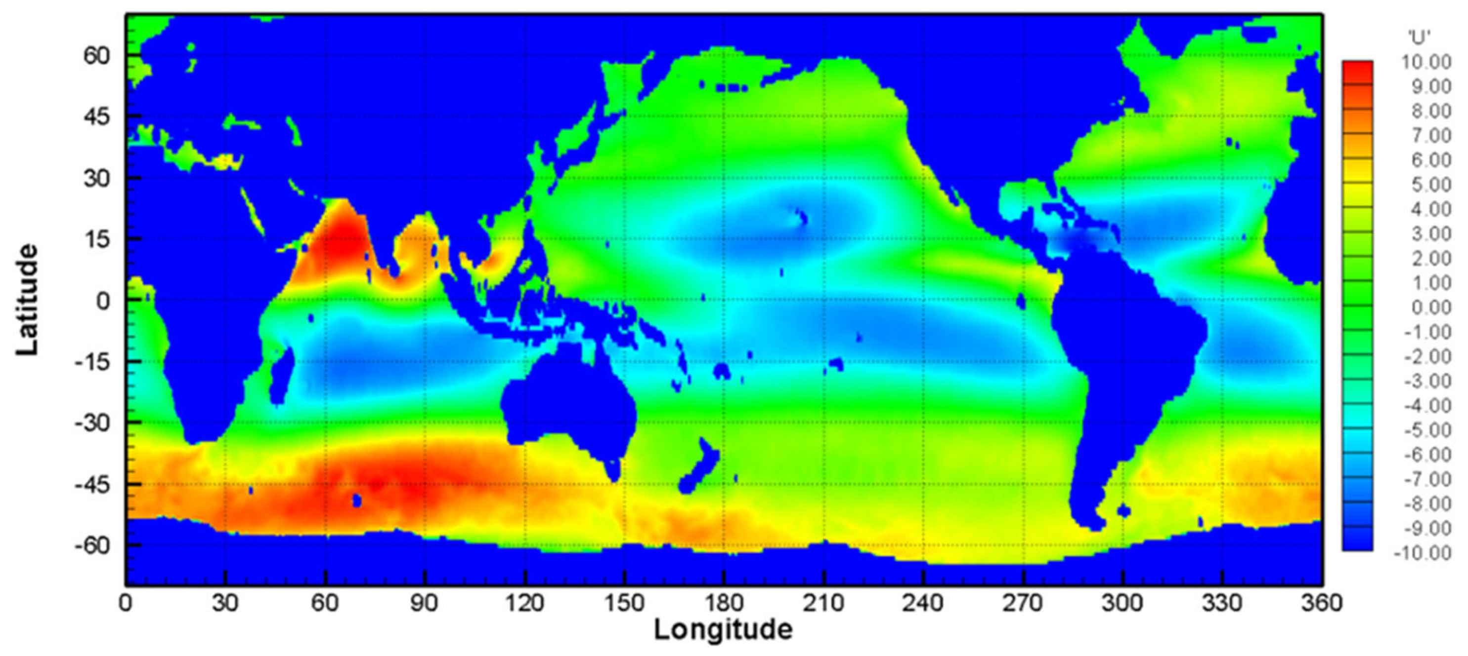
MATLAB was used to extract wind field data in NetCFD (*.nc) format, which contains information on several variables, including global variables. The data had a fixed height (sea level of 10 m) within the latitudes of −70° to 70° and longitudes of 0° to 360°. The wind direction and wind speed data were processed separately; thus, six variables were generated after the long-term data were processed. These data were stored as matrices for longitude (1440 × 1), latitude (560 × 1), time in months (12 × 1), radial wind (1440 × 560 × 12), zonal wind (1440 × 560 × 12), and wind speed (1440 × 560 × 12).

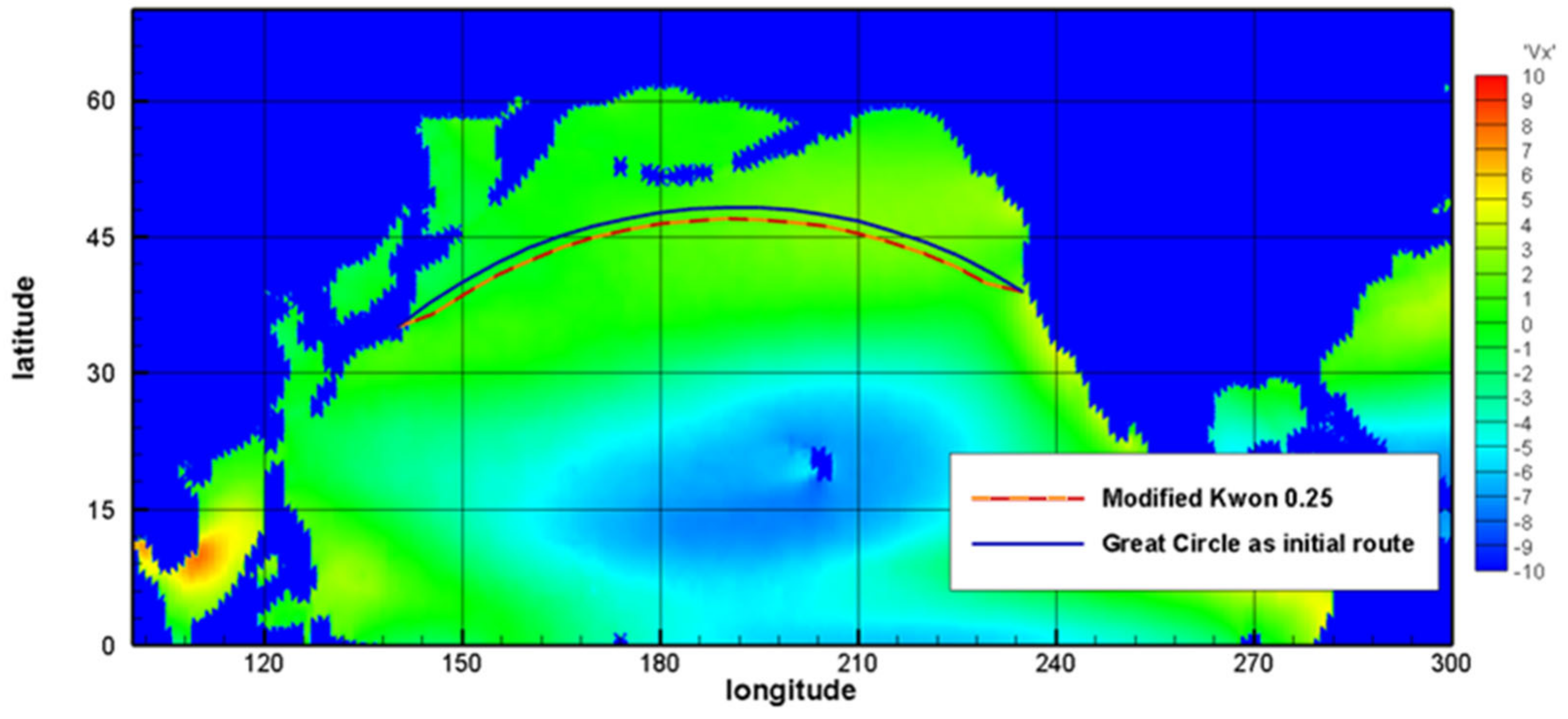
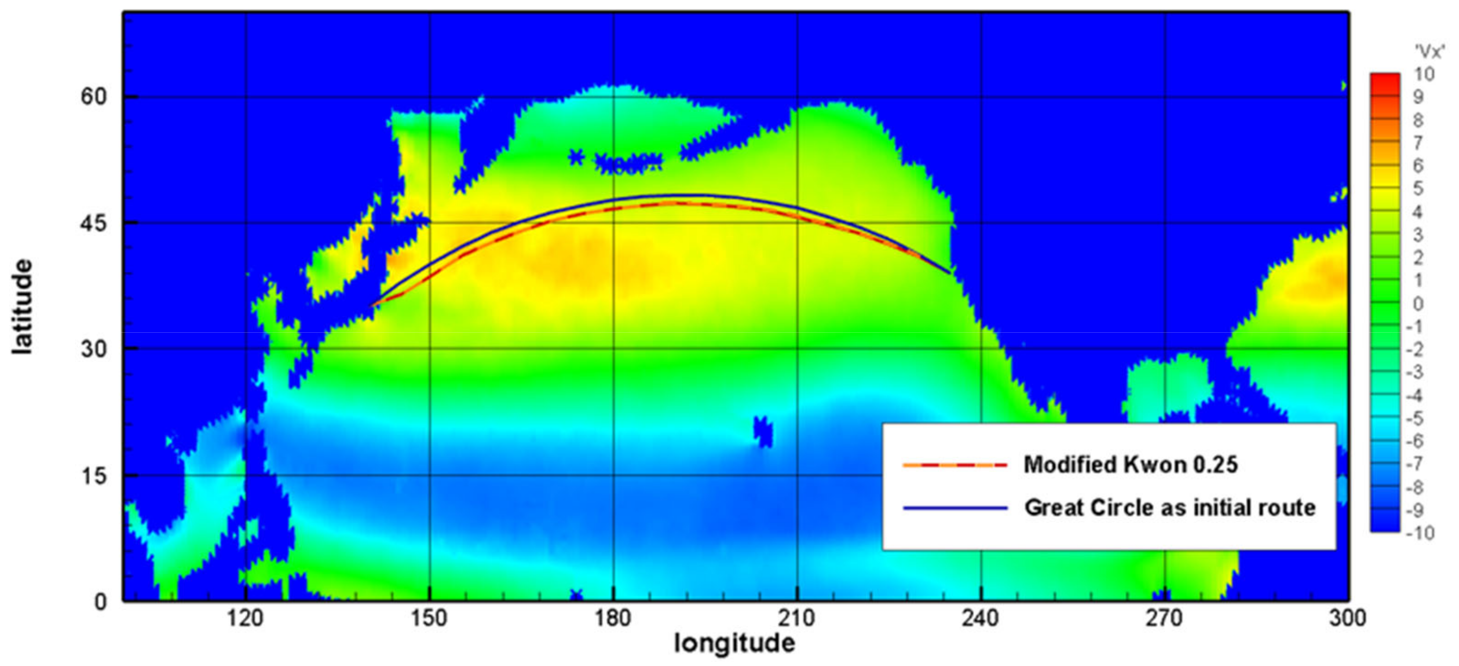
These data were exported and plotted using the Tecplot software to produce charts. For example, the horizontal and vertical components of the wind fields for July and December are presented in Figure 6 and Figure 7. The colors represent wind speed in knots plotted on a 0.25° × 0.25° grid. Wind field data were not available for the land area and are colored in blue.

For dynamic weather routing, wind field data were obtained at 3-h intervals on a 0.25° × 0.25° grid from the website of the European Center for Medium-Range Weather Forecasting.

In static weather routing, the weather information is obtained once. In contrast, weather information changes according to the weather forecast in dynamic weather routing. Figure 6 and Figure 7 illustrate the weather conditions along the route.

3.2. Dynamic Programming

The optimal shipping route typically depends on ship type, cargo, schedule, and operational plans when underway. In practice, these objectives must be considered together. Hence, multiobjective algorithms should be used for weather routing.

Dynamic programming is an effective method for solving multiobjective problems, such as the shortest path problem. Based on Bellman’s principle of optimality [36], dynamic programming simplifies a complex optimization problem by breaking it down into a sequence of smaller, more manageable problems. The most salient feature of dynamic programming is multistage optimization [37]. The ultimate goal of applying this weather routing approach is not to avoid all adverse weather conditions but to minimize sailing time while ensuring the safety of the vessel and crew.

In dynamic programming, each stage of the decomposed problem is optimized individually, with the solution from one stage serving as the input for the next. In this study, voyage progress was selected as the stage variable; each stage represented the journey between two waypoints in the problem’s planning horizon. The nodes selected at each stage constituted the decisive variable, and the objective was to minimize overall sailing time.

Another feature of dynamic programming is that each stage of the optimization problem has an associated state. Nodes govern the set of all possible choices for each stage. An increase in the number of nodes increases the computational cost. Node construction requires insight into the optimization problem; no rules for determining the nodes are available. In this study, nodes were selected as course turning points (i.e., waypoints) computed along a line perpendicular to the Great Circle route from the origin to the destination. Each course between stages could be expressed explicitly.

A recursive optimization procedure must be used to solve the overall problem by solving each stage in turn. This can either be a forward induction process from the origin to the destination or a backward process. Problems involving uncertainty, such as the shortest path problem, can only be solved with backward induction.

Recursive optimization was used to calculate the shortest sailing time between subvoyages. Weather forecast quality was considered to be lower for longer forecast times and more adverse weather. In practice, sailing routes should be recomputed whenever the meteorological data and the ship’s position are updated.

3.3. Formalizing the Dynamic Programming Approach

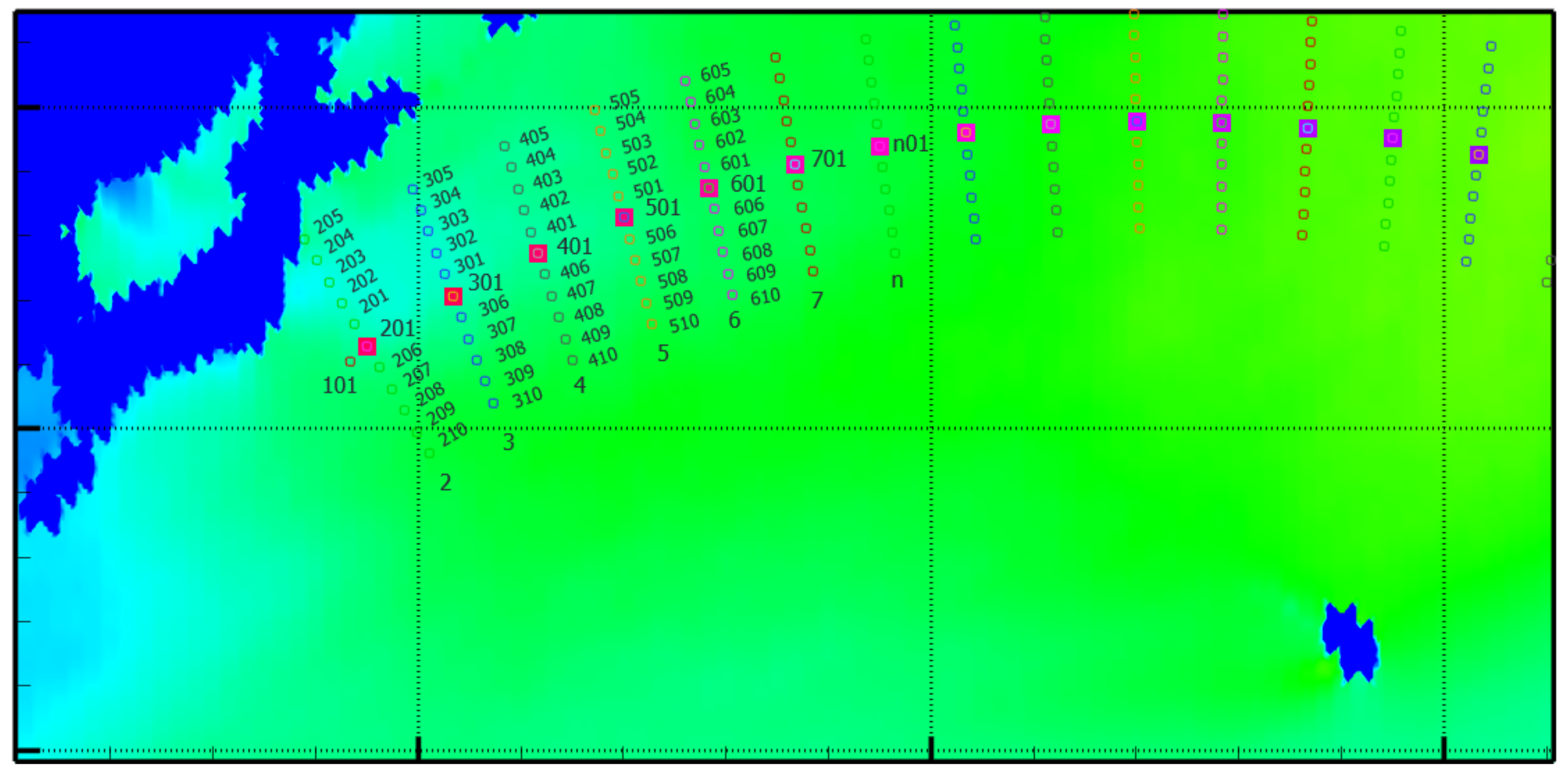
To plan a route based on meteorological information, an initial route must first be established. Multiple waypoints (i.e., nodes) can then be selected along the path. The route can be optimized by selecting a set of nodes. Figure 8 presents a grid system displaying a route between Japan and the US.

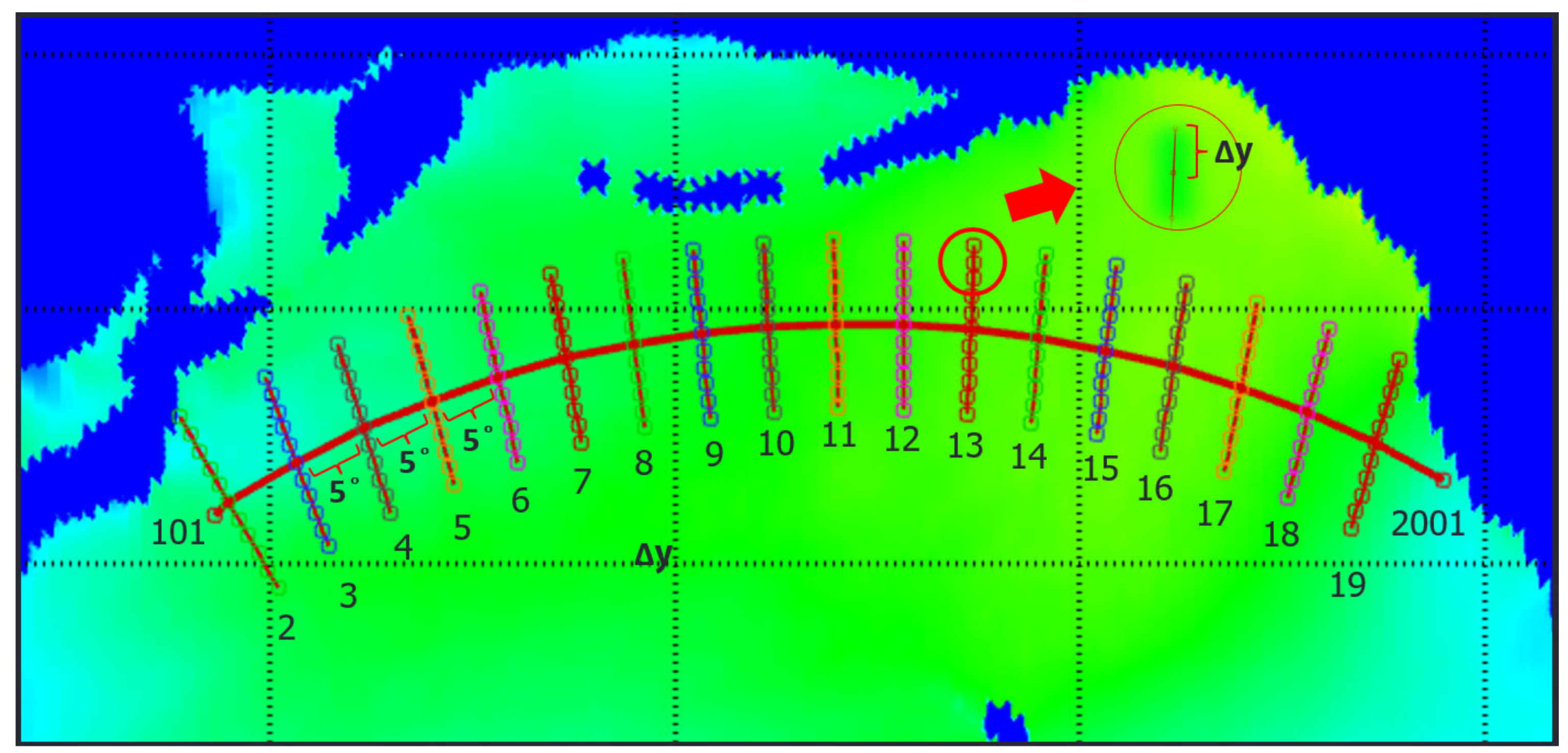
For the initial route, nodes were inserted every 5° of latitude from the origin (node 101) to the destination (node 2001), forming a 20-leg route with 19 decision stages. The nodes at each stage were perpendicular to the initial route, and the distance between adjacent nodes was $∆\mathrm{y}$. Figure 9 shows the numbering system for the nodes used in all the simulations.

Route adjustments should be made based on the vessel’s planned speed and any expected effects of tidal streams and currents. The quantity and spacing of the nodes at all stages are variables that can be determined on a case-by-case basis by considering the user’s preferences in the voyage area, the user’s total voyage distance, and the available computational capacity.

4. Case Studies

Two container ships were selected, and numerical simulations were performed on them to demonstrate the application of the proposed weather routing system.

4.1. KCS Simulation

To validate the prototype of the proposed weather routing system, simulations were performed on a KCS with a cargo-carrying capacity of 3600 twenty-foot equivalent units on an eastbound trans-Pacific voyage from Yokohama, Japan (φ 35°00.0′ N, λ 140°00.0′ E) to San Francisco, US (φ 39°00.0′ N, λ 125°00.0′ W) using static wind speed and direction data in July and December, respectively.

For a ship, the Great Circle route is a natural choice as the initial route because it represents the shortest distance. Waypoints were defined for this Great Circle route at intervals of 5° longitude for a total of 19 stages. A total of 11 nodes were defined for each stage, perpendicular to the route, with a separation of 0.25°, and on a straight line (i.e., a constant course in the Mercator projection). This initial route was optimized by selecting optimal nodes.

The optimized routes obtained after using the modified Kwon’s method are presented. Magnified maps for July and December are presented in Figure 10 and Figure 11. The average monthly wind speeds were significantly different in the northern oceans between July and December; the wind speed increased from summer to winter by more than 50% above 40° N. Therefore, compared to summer, there is a tendency to favor routes at higher latitudes in winter.

4.2. Container Ship Simulation

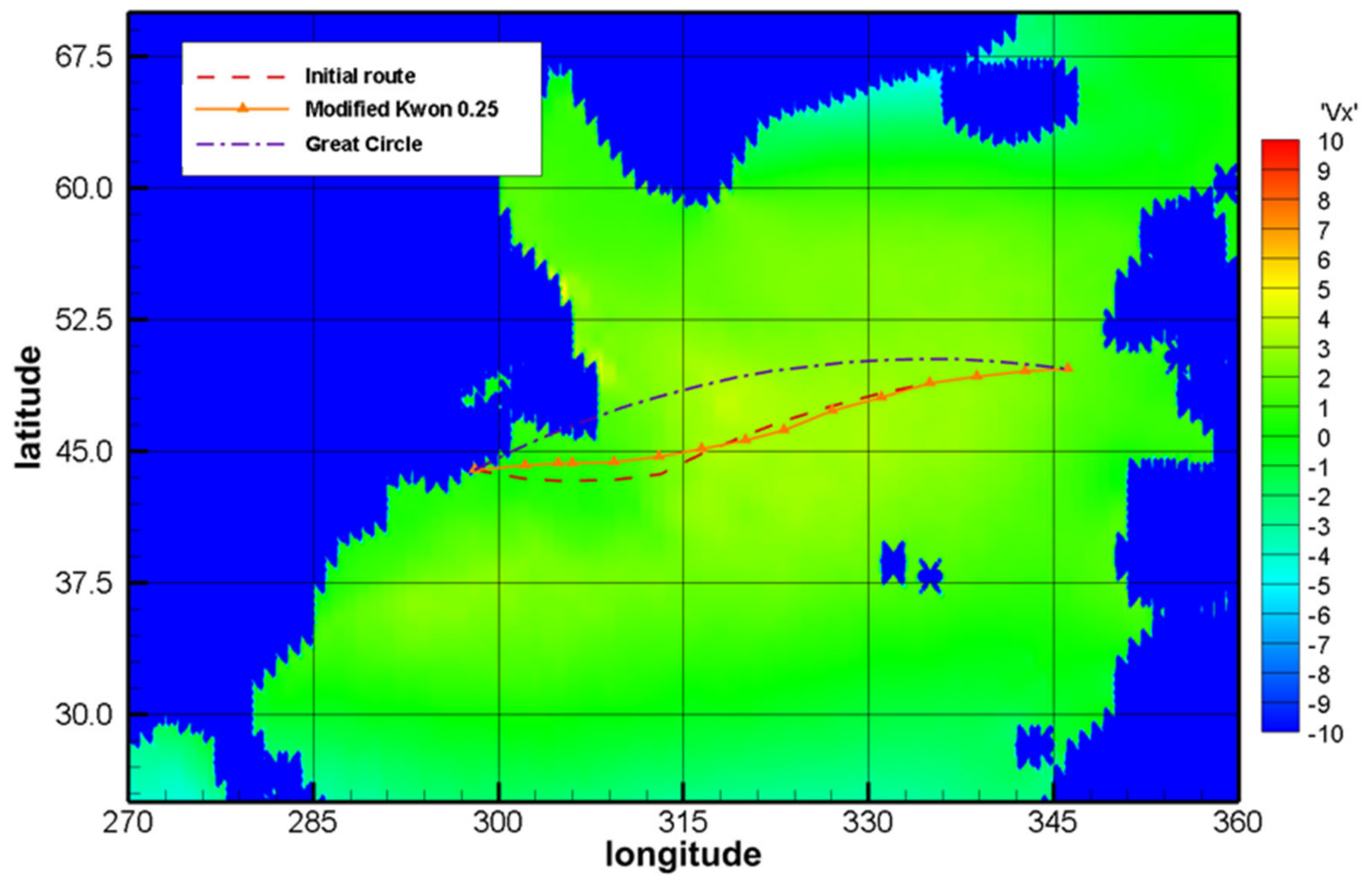
This study conducted additional simulations on a container ship with a cargo-carrying capacity of 4600 twenty-foot equivalent units on eastbound and westbound trans-Atlantic voyages. The eastbound voyage was from Halifax, Canada (φ 44°39.0′ N, λ 63°34.0′ W), to Rotterdam, the Netherlands (φ 51°55.0′ N, λ 4°28.0′ W). The westbound voyage was from London, England (φ 51°30.0′ N, λ 0°07.0′ W), to Norfolk, US (φ 36°51.0′ N, λ 76°17.0′ W).

In addition to the Great Circle routes, historical operating routes can be selected as the initial route in the proposed system. The course alteration points were derived from empirical data on course changes along the route. The container ship’s daily noon reports and voyage log in April were used to select the initial stages and nodes.

For the eastbound route, pilot time and estuary sections were deliberately removed from the optimization. The points (φ 43°93.0′ N, λ 61°90.0′ W) and (φ 49°69.0′ N, λ 13°80.0′ W) in the open sea were therefore selected as the origin and destination, respectively, resulting in a 15-stage dynamic programming problem.

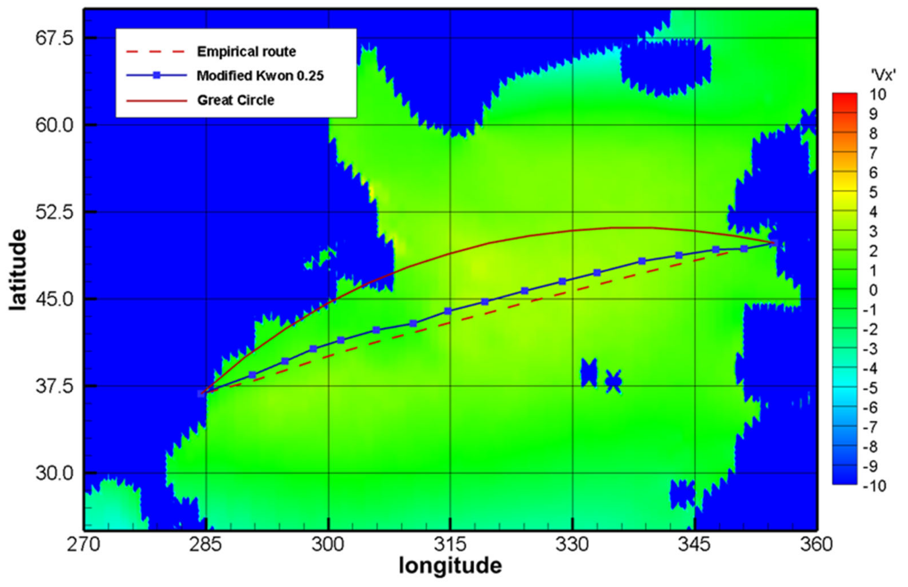
Dynamic wind speed and direction data for the North Atlantic were sourced from the European Center for Medium-Range Weather Forecasting and used to calculate ship speeds and headings between stages. Each stage, excluding the departure point, had a total of 17 nodes. Figure 12 depicts the initial historical route and the optimal routes obtained through the modified Kwon’s method. The Great Circle route is included for reference only.

Table 17. Comparison of ship operational performance between the selected optimal routes and the initial route of the voyage from Halifax to Rotterdam in April.

	Optimal Route (Speed Calculated by Modified Kwon’s Method)	Initial Route
Distance (miles)	4015	4109
Voyage Duration (days)	7.5	7.8
% of voyage duration compared to the initial route	−3.8	0

presents a comparison of the optimized routes and the initial routes. The modified route had a 3.8% lower travel duration than the initial route. Since we adopted a fixed fuel consumption approach, the percentage of fuel consumption savings is equivalent to time savings. This time reduction was achieved by choosing shorter routes when favorable weather conditions permitted and by preferentially sailing in calm water (i.e., sea state 0) without speed loss.

The return voyage was modeled with 17 legs and nine expansion nodes for each of the 16 stages. Figure 13 presents the initial historical route and the optimal routes obtained with the modified Kwon’s methods. According to data in

Table 18. Comparison of ship operational performance between the selected optimal route and the initial route of the voyage from London to Norfolk in April.

	Optimal Route (Speed Calculated by Modified Kwon’s Method)	Initial Route
Distance (miles)	6200	6298
Voyage Duration (days)	11.6	11.7
% of voyage duration compared to the initial route	−0.85	0

, the modified Kwon’s method reduced the voyage duration by 0.85% compared to the historic route of the liner. This study determined that the proposed method was consistent with the judgment of the captain who chose this empirical route.

5. Conclusions

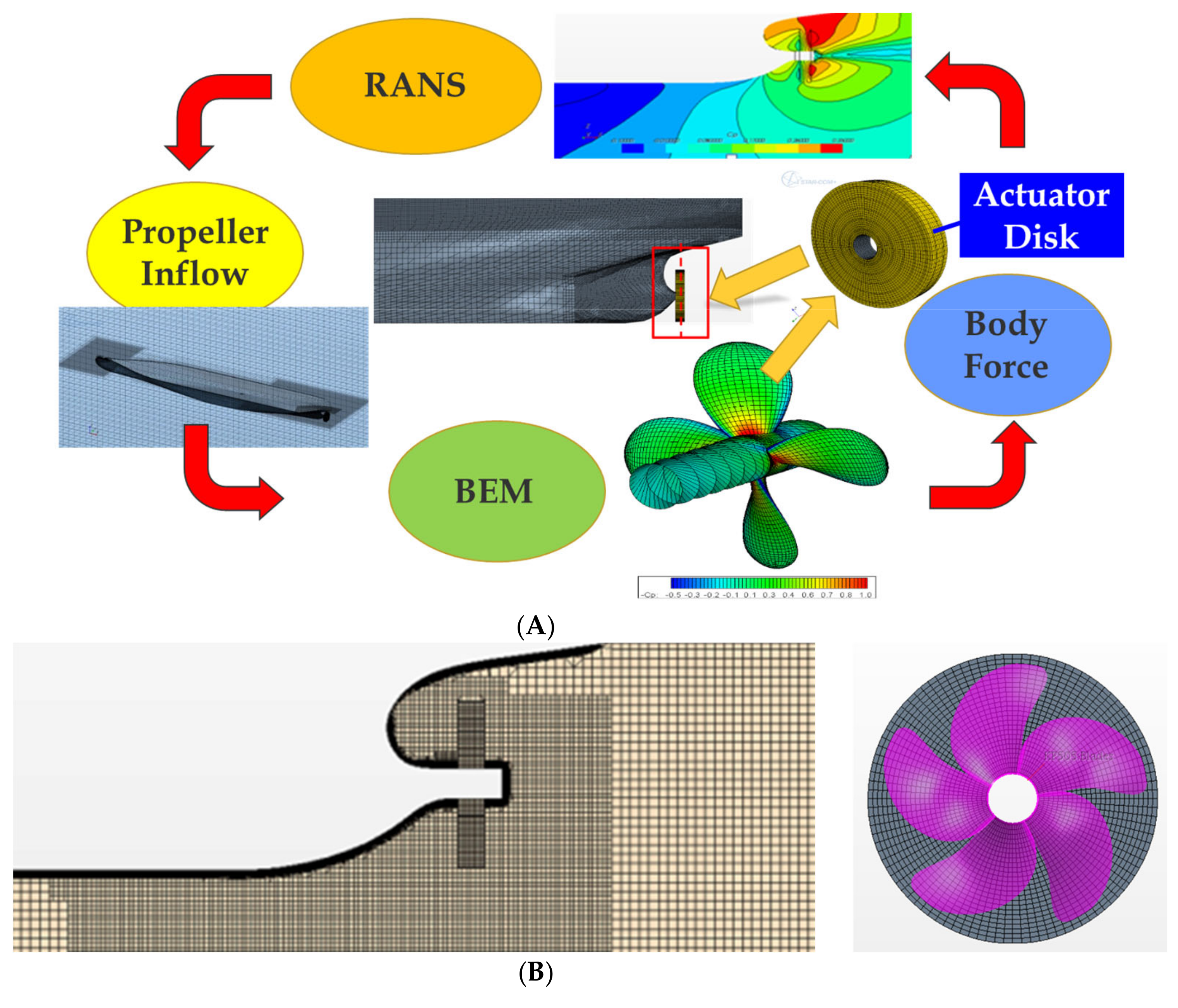
Rough weather conditions can substantially affect a ship’s performance. To mitigate the adverse effects, this study applies a multi-fidelity computational approach that integrates potential flow and viscous flow methods to calculate speed loss accurately and efficiently. Based on the computational results, the study modified the equations of the ship form coefficient $C_F$ in Kwon’s method to estimate the voyage performance of specific ship types under given wind conditions accurately and efficiently. This modified Kwon’s formula was integrated with an optimization system for weather routing. The utility of the proposed system was confirmed in two case studies involving container ships, wherein the proposed system suggested appropriate routes. This system could serve as a valuable resource for related research in the shipping industry.

The speed loss of the KCS at sea was evaluated using three methods: Kwon’s method, the MEPC method, and CFD simulations. Following empirical modifications, Kwon’s formula provided a closer approximation of speed loss, with derived results matching the numerical outcomes. While the modification proved effective, future research should focus on generating additional validation data for simulations under various wave conditions, including different Beaufort numbers. Furthermore, results for other ship models should also be gathered to facilitate broader comparisons.

The system could also be adapted to address operational requirements beyond voyage time reduction. For instance, cruise ships and chemical tankers carrying volatile cargo prioritize arriving safely on schedule, while schedule adherence is less critical for the other ship types. For North Atlantic container ships, minimizing fuel consumption is often the primary concern due to high fuel costs. In the future, the system could be extended to support multiobjective optimization, encompassing factors such as fuel consumption, operational costs, emissions, ship speed, and other considerations. Such advancements are now feasible, given the availability of affordable, high-performance computing resources.