Abstract
Pore connectivity and ultimate imbibed porosity are two important parameters used to assess the shale oil reservoir property, the proper appraising of which could facilitate the efficient flow of oil from the matrix and an improvement in recovery efficiency. In previous studies, the uncertainty in sample dimensions and the extra-long stable time during imbibition experiments exploring pore connectivity and ultimate imbibed porosity showed a lack of discussion, which influenced the accuracy and efficiency of the SI experiments. In this study, SI experiments with shale samples of different thicknesses are carried out to acquire the two parameters in a short period of time. As a result, the pore connectivity of sample D86-5 from the Qingshankou Formation (Fm) in the Songliao Basin fluctuates with the increase in thicknesses, with an average of 0.265. The water penetrates sample D86-5 of all thicknesses, so the ultimate imbibed porosity fluctuates around 3.7%, and the stable time increases with thicknesses. The pore connectivity of sample Y172 from the Shahejie Fm in the Bohaiwan Basin fluctuates around an average of 0.026, which is much smaller than that of D86-5. The ultimate imbibed porosity of Y172 decreases with thicknesses because the penetration depth is so small that the pores cannot be fully accessed, and the stable time increases before becoming stable with fluctuations. The method is examined using the samples from the Liushagang Fm in the Beibuwan Basin measuring around 400 μm: the ultimate imbibed porosity of BW1-1 and BW1-3 is 5.8% and 18.1%, respectively, the pore connectivity of BW1-1, BW1-2, and BW1-3 is 0.086, 0.117, and 0.142, respectively, and the results can be obtained within a day. In comparison, the average pore connectivity of the 400 μm samples from Qingshankou, Shahejie, and Liushagang Fms is 0.324, 0.033, and 0.097, respectively, and the average ultimate imbibed porosity of these Fms is 3.7%, 3.1%, and 12.0%, respectively. Based on the above results, a quick method for measuring the two parameters with thin samples by spontaneous imbibition is established, providing a fast solution for the evaluation of the sweet spot.
1. Introduction
With the growing demand for fossil fuels and the diminishment of conventional reservoirs, unconventional reservoirs, such as shale oil reservoirs, have grabbed the attention of researchers worldwide [1]. Shale reservoirs hold abundant oil, but they have low porosity and permeability, which impacts the high-efficiency exploitation of their resources [2]. The pore network is the storage space of shale oil; connected pores contribute to the fluid flow channel, whereas unconnected pores are called dead pores [3,4]. The pore connectivity of connected pores is a key factor influencing the flowing capacity of shale oil because good pore connectivity has the potential to realize high yield [5,6]. Some petrophysical methods have been used to investigate the pore connectivity of hydrocarbon reservoirs, such as mercury intrusion porosimetry (MIP), fluid tracing, wood’s metal impregnation, spontaneous imbibition (SI), and so on [7,8,9,10,11,12]. Imbibition commonly occurs in the process of exploiting shale oil/gas, referring to the phenomenon of the wetting phase penetrating into the non-wetting phase of shale rocks spontaneously, which is triggered by capillary force [13]. Comprehensively, in the research of pore connectivity, SI is readily implemented compared with other methods, where the slopes of imbibition curves reflect pore connectivity; however, it requires a considerable amount of time to complete. In some studies, imbibition could take more than 600 h before reaching a stable status, and it is hard to determine whether the imbibition fluid has entered all connected pores [14,15]. Therefore, it is critical to raise the efficiency of SI tests on shale rocks by reducing the imbibition time.
Apart from pore connectivity, the ultimate imbibed porosity of shale rocks during imbibition is also a crucial parameter when appraising the potential of a shale reservoir, which is reflected by the water volume that can penetrate the rock by the time when the imbibition curve reaches a stable status [16,17]. During the process of imbibition, the wettability of shale rocks plays a significant role in the affinitive ability of the rocks to a certain kind of fluid [18]. When oil-wet pores are predominant in the rock, the rock demonstrates a preference for oil instead of water, and vice versa, thereby influencing the volume of the water entering the rock. Therefore, ultimate imbibed porosity is also affected by the wettability and the pore structure [19,20]. When the ultimate imbibed porosity is large in the imbibition process, the efficiency of enhanced oil recovery (EOR) can be improved, which is a set of techniques employed to increase the amount of crude oil that can be extracted from an oil field after the primary and secondary recovery methods have been exhausted [21]. The main methods of EOR can be summarized into three techniques, i.e., solvent, chemical, and thermal, which are mainly involved with the injection of different substances that are not naturally found in the reservoir, where SI is highly engaged in and contributes to the displacement of oil by water [22,23,24]. By defining the ultimate imbibed porosity of shale rock, the recovery efficiency of the exploitation can be estimated.
To ascertain pore connectivity and ultimate imbibed porosity, a number of experiments were conducted in the past. Laboratory SI tests were widely conducted as a crucial method combined with other laboratory methods for the characterization of pore connectivity and ultimate imbibed porosity, for example, contact angle analysis, fluid tracing, nuclear magnetic resonance (NMR), mercury intrusion porosimetry (MIP), and so on [25,26,27,28,29]. Some studies were conducted extensively on different aspects of the pore structure, pore connectivity, and ultimate imbibed porosity of shale samples from a specific source, for instance, the influence of changing the imbibition liquid on the matrix, the flowing feature of the tracer fluid in the shale matrix, or the comprehensive analysis of the shale in a particular location [27,30,31,32,33], but the dimensions of the samples selected in the research were out of focuses. In addition, some researchers observed that the distinct depths at which tracer fluids permeated into the rock from the solid–liquid boundary during SI reflected certain differences in the imbibition results [34], which also stressed the importance of defining the thickness of the tested shale rock. Apart from that, by constructing a three-dimensional (3D) pore structure with stacking scanning electron microscopy (SEM) images of an Eagle Ford sample, Davudov et al. discovered that the amount of connected pores decreases with an increase in the thickness of digital samples by modeling, showing the effect of thickness [35]. By setting samples with different thicknesses and origins, the identification of the penetration depth of certain shale rocks during SI could not only improve the scientific research on the shale structure but also provide a possibility for the productive practical exploitation of shale oil/gas [36].
The results of SI tests on ultimate imbibed porosity and pore connectivity are also influenced by mineral components and the amount of organic matter. Mineral components and TOC were also found to remarkably influence the shale pore structure. Clay minerals tend to form more complex pores compared with brittle minerals like quartz, which create larger pores [15,37,38]. When SI happens, the clay in shale swells, and cracks are created, making it more efficient to exploit shale oil/gas [14]. TOC is essential in describing the organic matter in the pore space, which helps in shaping the pores in the early stage of layer formation [39].
Based on the previous studies, this research was designed to explore the following problems: the extremely long time of imbibition tests, the difficulty in the measurement of pore connectivity and ultimate imbibed porosity, and the unknown influence of parameter thickness during SI.
By conducting SI tests with samples of different thicknesses, this research aims to explore how the penetrating process during SI is related to thickness and to further analyze the pore connectivity, ultimate imbibed porosity, and their distributions according to different formations. Samples from the Qingshankou, Shahejie, and Liushagang Fms were chosen and evenly sliced into cylinders in certain thicknesses and approximately the same diameter, covering onshore and offshore shale rocks. In this study, a quick method for evaluating the pore connectivity and ultimate imbibed porosity of the shale matrix using small-thickness samples was established, introducing thickness as a critical parameter and emphasizing the significance of length control in future assessments of pore structure. Utilizing this method, the pore connectivity and ultimate imbibed porosity of all samples were observed to vary with thicknesses.
2. Sample Background, Experimental Methods, and Theory Preparation
2.1. Sample Background and Experimental Methods
Shale samples were chosen from Qingshankou Fm in Songliao Basin, Shahejie Fm in Bohaiwan Basin, and Liushagang Fm in Beibuwan Basin. The Liushagang Fm samples were collected from offshore drilling boreholes, and the samples from other formations were onshore cores. Some experimental methods were conducted in this research, including FEI Helios Nanolab 650 dual beam FIB and SEM, Rigaku TTR III diffractometer, ELTRACsi, and Mettler Toledo ME204, from which the SEM pictures and the basic properties of the samples, as well as the SI test results, were obtained accordingly.
The ion-milled mudstone blocks were tested by Zeiss GeminiSEM450 and FEI Helios Nanolab 650 dual beam FIB-SEM to detect the mineral and organic matter particles and pore spaces with a working distance of 10 mm, following the methods of SEM equipment and sample preparation in prior studies [40,41]. The mineral properties were tested by the Rigaku TTR III diffractometer, while the TOC content was examined by ELTRACsi, presenting the mineral content and the content of organic matter in the examined samples. In the meantime, the samples of each origin were sliced into cylinders, whose thicknesses increased at an interval of approximately 200 μm from about 400 to 2000 μm, which varied with the different conditions of the samples, as can be seen in Figure 1. The minimum thickness of 400 µm represented the finest increment achievable by the cutting machine and was therefore selected as the starting point for the increasing thicknesses. Given that liquid penetrates from both sides of the samples, it was theoretically expected that with each 200 µm increase in thickness, there would be a corresponding 100 µm increase in the depth of water penetration. A final thickness of 2000 µm was chosen, but more samples of larger thicknesses are expected in future studies in case the liquid cannot penetrate. The thicknesses and volumes of the samples are listed in Table 1. The cylindrical samples whose thicknesses were >1400 μm had their flank covered with epoxy adhesive in order to prevent the imbibition liquid from injecting via the flank side. The imbibition liquid in this research was deionized water, reducing the influence of other impurity substances.
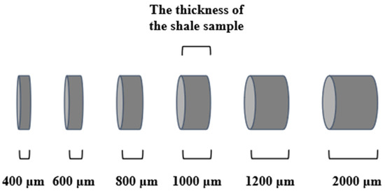
Figure 1.
The target thickness of shale samples, from 400 μm to 2000 μm.

Table 1.
The thicknesses and volumes of the samples.
The cylindrical samples were placed and examined in the equipment below, which was improved based on a former research study [16], as shown in Figure 2a, consisting of a data-recording computer and a thermostatic testing part. A balance (Mettler Toledo ME204) is attached to a small beaker and connected to the computer so that the data of the content in the small beaker can be recorded every minute (see Figure 2a). The samples are put into the small beaker that hangs in a bigger beaker filled with imbibition liquid using a fishing line. The equipment is connected to the balance so that the recorded data represent the weight of the imbibed water. This method guarantees that even if any fragments of the samples fall, the small beaker makes sure that the data are not affected. Dissimilar to the sample placement of the previous research, which has no requirements for the samples’ positions, the samples are placed perpendicularly to the bottom of the small beaker, with supports on both undersides of the cylindrical samples, ensuring that the gaseous phase products generated during the imbibition can be removed in time.
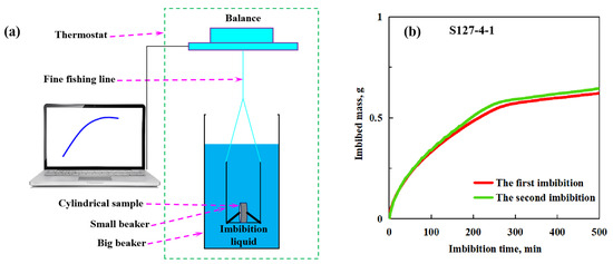
Figure 2.
The equipment and repeated group of spontaneous imbibition experiments: (a) the equipment; (b) the repeated group of sandstone sample S127-4-1.
The imbibition method was tested with repeated groups of a sandstone sample, and the change in the mass of sample S127-4-1 during two SI experiments is exhibited in Figure 2b. It can be seen that the imbibition curves between two SI experiments on the same sample are highly similar, which proves that the method in this research can be repeatable. In comparison, the sliced shale samples tested in repeated groups have more fluctuations than the sandstone samples. This is because the heterogeneity in shales and the expansion of the clay content influence the imbibition curves, making the SI experiments of thin shale rocks less repeatable [42].
2.2. Theory Preparation
Washburn [43] found that the pores of porous materials can be seen as cylindrical capillaries, and at the end of time t (in s), the volume of the liquid (V, cm3) that enters into n cylindrical capillaries with radii r1, r2, …, rn can be presented as:
where l is the length of the capillary tube, cm; η is the viscosity of the intruding liquid, mP; PE is the total external pressure the liquid receives from the back, MPa; and γ is the surface tension of the liquid, Newton per cm. If the pressure of the liquid is constant and small relative to γ/η, this equation can be simplified as:
where k′ is a constant that is relevant to the total pore diameter, and the latter also remains unchanged in the same sample during imbibition, so it is not involved with the characteristics of the liquid. In this way, the volume that penetrates a porous body within SI is proportional to the imbibition time t, s.
Furthermore, the Handy equation [44] is widely used to describe the imbibition process. The Handy equation assumes that the liquid imbibes as pistons in a vertical direction, neglecting the gas pressure gradient in the front of the imbibed liquid. The equation is presented as follows:
where is flow rate, cm3/cm2/sec; kw is the effective water permeability, D; is the water viscosity, centipoises; Pc is the capillary pressure, MPa; is the density difference for water and air; g is the acceleration due to gravity; x is the position of front, cm; and Pc is a constant. When there is piston displacement,
where is the fractional porosity; Sw is the fractional water content of pore spaces; and t is the imbibition time, s. Combining Equation (3) and Equation (4), the result would be:
When the gravity force is dramatically smaller than the capillary force and , the equation would become:
where Qw is the total imbibed liquid, cm3; Pc is the capillary pressure, MPa; is fractional porosity, %; kw is effective water permeability, D; Ac is the cross-sectional area of the sample, cm2; Sw is the fractional water content of the pore spaces, %; μw is the water viscosity, mP; and t is the imbibition time, s. When the buoyancy effect of the sample volume needs to be removed to obtain the imbibed porosity, this equation can become:
where Qd is the volume of the dry sample, cm3, and a is the quality of the sample that is not influenced by other conditions but by the nature of the shale. In this equation, Qw/Qd represents the imbibed porosity per unit volume of the samples, %, and a represents the pore connectivity of the shale sample. This provided simplified and concrete evidence to investigate spontaneous imbibition, leaving the imbibed porosity and time in a linear relationship.
The slope of the curve showing the changes in imbibed porosity with time (Equation (7)) reflects the pore connection of the samples [27,45]. In this research, pore connectivity is normalized to mitigate the impact of thickness, which is a critical parameter:
where an is the pore connectivity, a is the slope in the linear fitting of the imbibition curve, which is called the initial imbibition rate, and T is the thicknesses of the samples, cm. The slope was normalized by multiplying half of the length of the corresponding sample since the injection of imbibition liquid occurs from both undersides of the cylinder sample.
3. Results and Discussion
3.1. Basic Properties and Material Components
The measured basic properties and material components of the samples are presented in Table 2, where the percentages of the figures signify the mass percentages of the properties versus the whole samples. The samples are from different origins, and their depth varies from 1957.6 m to 3561.9 m. The lithofacies of samples include mixed and clayey shales. Sample D86-5 from the Qingshankou Fm is clayey shale, and sample Y172 from the Shahejie Fm is mixed shale. The samples from the Liushagang Fm have both clayey and mixed shales, such as BW1-1 and BW1-2 belong to mixed shales, and BW1-3 belongs to clayey shale. Quartz is widely seen in the mineral content of all selected samples; sample BW1-2 holds the highest quartz content of 37.1%, and sample BW1-1 holds the lowest content of 18.3%, showing a great divergence because of the heterogeneity in the samples. The feldspar content in all samples is at a lower level compared with the quartz content, which is the highest in sample D86-5 at 13.7%. Sample Y172 and samples BW1-1, BW1-2, and BW1-3 all have lower contents of feldspar (1.9%, 1.3%, 1.7%, and 0.9%, respectively). The calcite content of sample BW1-1 is the highest at 32.6%, which is dramatically distinct from the other two groups of samples that are also from the Liushagang Fm (BW1-2 and BW 1-3), whose content of calcite is much smaller, at 6.8% and 0.2%, respectively. Sample Y172 from the Shahejie Fm contains 27.4% calcite content, which is also relatively high. Samples D86-5 and BW1-3 contain no ankerite, while sample Y172 shows the highest ankerite content in all samples (20.6%). The siderite and pyrite content of the samples are in the range of below 10%, and the divergence between the different samples is not as significant as the other minerals. The clay content of most samples has a relatively large percentage. Sample D86-5 from the Qingshankou Fm and samples BW1-1, BW1-2, and BW1-3 from the Liushagang Fm are all abundant in clay minerals, at 46.8%, and an average of 41.23%, respectively. Sample Y172 from the Shahejie Fm holds a lower clay content of 24.7%. The TOC content of all the samples is in the range of 2.2% to 5.8%. The samples from the Liushagang Fm have a relatively high level of TOC content (2.7%, 5.8%, and 3.9%, respectively) but vary considerably despite the same origin, while the samples from Qingshankou and Shahejie Fm show a lower level of TOC (2.2% and 3.0%, respectively). In general, the quartz, calcite, and clay content of the samples account for a higher percentage of all minerals, and the TOC content is distinct. The samples exhibit a remarkable nature of heterogeneity in the properties, and the SI test is notably influenced by the contents.
Table 2.
The basic properties of the samples.
3.2. SEM Analysis
SEM images of the four formations are displayed in Figure 3, where the representative area of the samples in each origin is chosen to show the pore structure of the samples. In Figure 3a, the overall view of the examined sample from Qingshankou Fm is shown, where the existence of narrow long cracks extending for more than 30 μm and interparticle pores along with pyrite minerals is revealed. Figure 3c is the enlargement of the yellow square part of Figure 3b, both showing a substantial amount of organic pores, where the porous space difference in the two kinds of pores can be obviously seen, and the organic matter widely distributes among the minerals. Figure 3d is an image of the pore structure of the sample from the Shahejie Fm. Figure 3e,f are the enlargements of its yellow square parts, where large areas of organic matter along with narrow cracks and inorganic pores can be seen, and the organic matter represents a large portion of the shale rock. Figure 3g shows the prevailing existence of pyrite minerals and organic matter in the examined sample from the Liushagang Fm. Figure 3h,i are the enlargements of Figure 3g, showing that the mineral aggregated in the yellow square of Figure 3g is a mixture of pyrite and a mass of organic matter, with abundant micro-cracks alongside, and the mineral mixture contains plentiful pores with organic matter. Similar to what the basic properties of the samples exposed, the SEM images in Figure 3 demonstrate the pronounced heterogeneity characteristics of shale, which significantly impact pore connectivity and ultimate imbibed porosity [46,47].
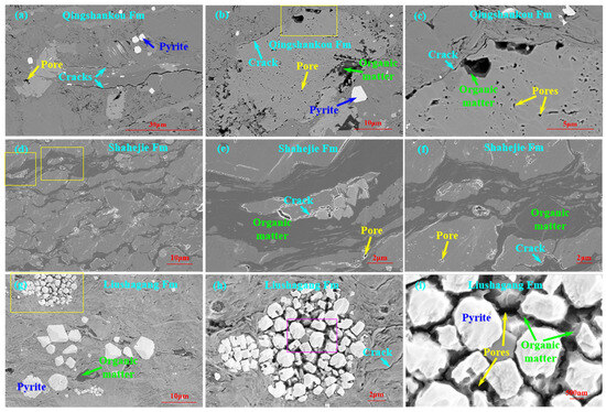
Figure 3.
SEM pictures: (a–c) Qingshankou Fm, (d–f) Shahejie Fm, and (g–i) Liushagang Fm. The square areas in yellow and purple are enlarged, as illustrated in the figures next to them.
3.3. Changes in the Imbibition Curves with Sample Thickness
After the imbibition tests, the imbibition data of various samples were collected and normalized to acquire the ultimate imbibed porosity. The peak of an imbibition curve was considered to reflect the ultimate imbibed porosity. In some cases, when the rate of water penetrating into the rocks becomes zero and the imbibition curve reaches a stable status with time [48], the time that the samples take is recorded as the stable time. The full time of the imbibition is processed into square root, and the linear-fitted slope of the initial imbibition curve is called the initial imbibition rate; after normalizing the initial imbibition rate, it can reflect the pore connectivity [34]. In this research, samples with different thicknesses were used. To compare the pore connectivity from samples of different thicknesses, the pore connectivity was normalized by considering the thicknesses of rocks.
Figure 4 illustrates the imbibition curves of sample D86-5 with different thicknesses with the unprocessed time in minutes, with different colors representing the results of different thicknesses. All the curves in Figure 4 show that the imbibed porosity increases rapidly with time, and a stable status is reached in all groups. The stable time of different samples can be affected by many factors, and in this case, it changes with thicknesses [15,48]. In Figure 4a, the stable time of the sample with a thickness of 450 μm is 46 min, which is the smallest in all samples. In Figure 4b–f, the stable time increases with the addition of thicknesses 640 μm, 750 μm, 1100 μm, 1270 μm, and 1940 μm, corresponding to the stable time of 72 min, 102 min, 350 min, 397 min, and 1361 min, respectively.
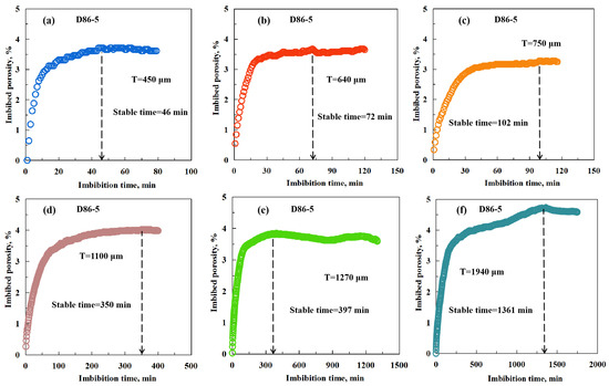
Figure 4.
The unprocessed spontaneous imbibition curves of sample D86-5 with different thicknesses: (a) 450 μm; (b) 640 μm; (c) 750 μm; (d) 1100 μm; (e) 1270 μm; and (f) 1940 μm.
The spontaneous imbibition curves of sample D86-5 with square-rooted time are shown in Figure 5, which includes different thicknesses of the sample in different colors. The imbibed porosity increases with imbibition time gradually in all the samples. In Figure 5a, the ultimate imbibed porosity and the initial imbibition rate are 3.8% and 1.441, respectively. In Figure 5b, the ultimate imbibed porosity and the initial imbibition rate are 3.7% and 0.849, respectively. In Figure 5c, the ultimate imbibed porosity and the initial imbibition rate are 3.3% and 0.589, respectively. In Figure 5d, the ultimate imbibed porosity and the initial imbibition rate are 4.0% and 0.441, respectively. In Figure 5e, the ultimate imbibed porosity and the initial imbibition rate are 3.8% and 0.382, respectively. In Figure 5f, the initial imbibition rate is 0.294 and the ultimate imbibed porosity is 4.7%
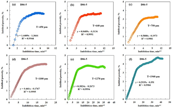
Figure 5.
The spontaneous imbibition curves of sample D86-5 with different thicknesses: (a) 450 μm, (b) 640 μm; (c) 750 μm; (d) 1100 μm; (e) 1270 μm; and (f) 1940 μm.
Figure 6 shows the imbibition curves of sample Y172 with different thicknesses with the unprocessed time in minutes. The characteristics of these curves are different from the previous curves (sample D86-5). In all the groups of sample Y172, the whole periods of imbibition fluctuate. In Figure 6a,c, the samples with thicknesses of 460 μm and 840 μm reach a stable status and continue to remain stable, with stable times of 730 min and 1297 min. In contrast, in Figure 6b,d,e, the samples with thicknesses of 680 μm, 1070 μm, and 1140 μm reach a stable status but decline immediately, with stable times of 1429 min, 1353 min, and 1246 min, respectively.
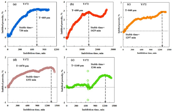
Figure 6.
The unprocessed spontaneous imbibition curves of sample Y172 with different thicknesses: (a) 460 μm; (b) 680 μm; (c) 840 μm; (d) 1070 μm; and (e) 1140 μm.
The imbibition curves of sample Y172 with square-rooted time are shown in Figure 7, which includes samples with different thicknesses. The processed imbibition curves reveal more fluctuation in the initial periods of imbibition. In Figure 7a, hardly any imbibition occurs in the initial period, which is mainly caused by the fact that it requires more interaction time between water and rock before liquid fills into shales. In Figure 7b, the initial imbibed porosity is about zero, which indicates that water has scarcely filled into the rock. Likewise, in Figure 7c, the initial imbibed porosity is also approximately zero and then increases gradually. In Figure 7d, the initial imbibed porosity has some fluctuation but is still near zero. In Figure 7e, the interaction time between the water and rock is long before the fluctuation period ends, and then water fills into the rock quickly. From Figure 7a,e, the ultimate imbibed porosity of sample Y172 is 3.1%, 2.8%, 1.4%, 1.3%, and 0.8%, respectively.
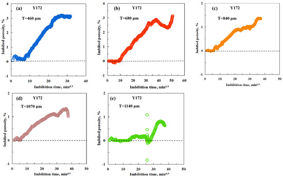
Figure 7.
The spontaneous imbibition curves of sample Y172 with different thicknesses: (a) 460 μm; (b) 680 μm; (c) 840 μm; (d) 1070 μm; and (e) 1140 μm.
At the initial time of the imbibition curves, some special phenomena appear, such as the imbibed rate staying at about zero, the imbibition curve decreasing, and the apparent imbibition porosity dropping to below zero, which influence the selection of the initial curve slopes. Therefore, a turning point aiming to remove the influence of abnormal phenomena during the initial imbibition time is chosen as the starting point for calculating the initial curve slopes. After the turning point, the imbibed porosity increases quickly until reaching stability or the point of declining. The modified imbibition curves of sample Y172 with different thicknesses are shown in Figure 8, whose starting points are adjusted to the turning point. The initial imbibition rates are 0.143, 0.088, 0.050, 0.042, and 0.031, respectively. Upon converting the initial imbibition rate into pore connectivity, the results are 0.033, 0.030, 0.021, 0.023, and 0.018, respectively.
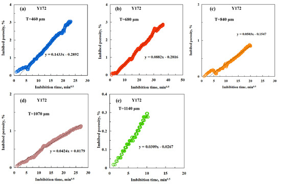
Figure 8.
The modified spontaneous imbibition curves of sample Y172 with different thicknesses: (a) 460 μm; (b) 680 μm; (c) 840 μm; (d) 1070 μm; and (e) 1140 μm.
The stable time, ultimate imbibed porosity, and pore connectivity of samples D86-5 and Y172 were obtained from the imbibition tests, and their variations with the thicknesses of the corresponding samples are shown in Figure 9. Figure 9a–c show the variation in the stable time, ultimate imbibed porosity, and pore connectivity of sample D86-5 with different thicknesses, while Figure 9d–f show those of sample Y172 with different thicknesses. In Figure 9a, the stable time of D86-5 gradually increases from 46 min to 1361 min with the added thicknesses, with an average of 388 min; the ultimate imbibed porosity varies from 3.3% to 4.0%, with an average of 3.7%, with the pore connectivity varying from 0.221 to 0.324, with an average of 0.265. In contrast, the stable time of sample Y172 initially increases from 730 min to 1429 min when the thickness increases from 460 μm to 680 μm and then remains at a high level, ranging from 1246 min to 1353 min, with an average of 1211 min, which is much higher than the average stable time of sample D86-5. The ultimate imbibed porosity of sample Y172 decreases dramatically with the increase in thicknesses, ranging from 0.8% to 3.1%, with an average of 1.8%, and the pore connectivity values all remain at an extremely low level, changing from 0.018 to 0.033, with an average of 0.026, which are also much smaller than those of sample D86-5.
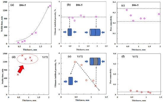
Figure 9.
The relationship between stable time, ultimate imbibed porosity, and pore connectivity and thickness: (a–c) sample D86-5 and (d–f) sample Y172.
The differences between the two groups of samples are due to their different pore connectivity values. In Figure 9b,e, the models show the influences caused by different pore connectivity, with blue representing the water and water-penetrated rock and grey representing the rock that water does not enter. Theoretically, as the natural characteristic of shale rocks, the pore connectivity of a shale rock is constant, so the penetration depth is also constant with an increase in thickness. In this study, the average pore connectivity of sample D86-5 was 0.265, which is almost ten times larger than that of sample Y172, despite some fluctuations. With better pore connectivity, water can completely penetrate sample D86-5, and the penetration depth is over 970 μm, which is half of the largest thickness of sample D86-5, because water enters from both sides of the sample. As a result, the ultimate imbibed porosity stays around the average value because all the connected pores are accessed. With a small pore connectivity, the penetration depth of sample Y172 is much smaller. In Figure 9d, the stable time increases dramatically from samples at 460 μm to 680 μm, so the penetration depth is between 230 μm and 340 μm. Thus, the ultimate imbibed porosity of sample Y172 declines with thickness because the volume of the sample has increased, but the water cannot enter the volume deeper than 340 μm. The complex pore structure of Y172 influences and declines the efficiency of water entering into the pores with the increase in sample thicknesses, resulting in a long stable time.
Due to the accurate value of pore connectivity and ultimate imbibed porosity relying on sample thickness, when determining these two parameters, the thickness of the sample should be considered. And when the pore connectivity is small, the ultimate imbibed porosity and stable time are influenced by not only the thickness but also the penetration depth.
3.4. The Imbibition Curves of the Offshore Shale Samples
Based on the results of the quick method of appraising imbibed porosity and pore connectivity, three offshore samples (BW1-1, BW1-2, and BW1-3) were tested to examine the method. Figure 10 exhibits the imbibition curves with the original imbibition time, the imbibition curves with the square-rooted time, and the modified imbibition curves with the square-rooted time, with different colors representing different samples, from which the stable time, ultimate imbibed porosity, and pore connectivity can be acquired. Samples BW1-1, BW1-2, and BW1-3 have thicknesses of 410 μm, 440 μm, and 400 μm, which can be seen as approximately the same value and are also the smallest thicknesses of a slice of shale rock the experiment machine could produce.
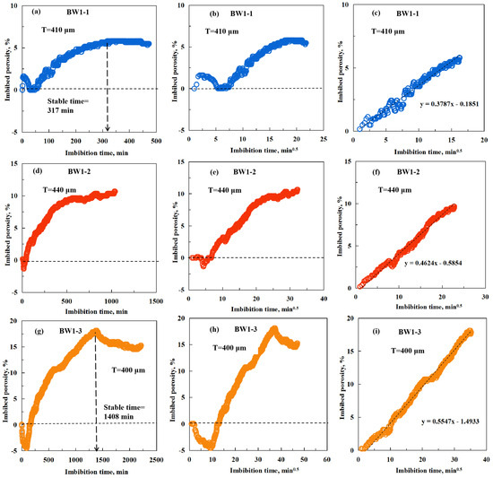
Figure 10.
The unprocessed spontaneous imbibition curves, imbibition curves, and modified imbibition curves of different samples: (a–c) BW1-1 with a thickness of 410 μm; (d–f) BW1-2 with a thickness of 440 μm; and (g–i) BW1-3 with a thickness of 400 μm.
In Figure 10a,d,g, the fluctuations are obvious in all three samples during the whole imbibition process, and sample BW1-2 does not reach a stable status until the end of imbibition. The stable times of BW1-1 and BW1-3 are 317 min and 1408 min, respectively, which are shorter than a day’s time. In Figure 10b, the imbibition curves with the processed time increase sharply and then decrease quickly. This phenomenon is mainly caused by imbibition-induced cracks, which are caused by clay expansion. Induced cracks are mainly oil-wet and increase the buoyancy of the samples, making the imbibition curves decrease. In Figure 10e, the imbibition curve almost remains stable in the initial period because it requires the interaction time, and then it decreases because of the imbibition-induced cracks. In Figure 10h, the imbibition curve decreases quickly in the initial period, which is also caused by the imbibition-induced cracks. The ultimate imbibed porosity of BW1-1 and BW1-3 is 5.80% and 18.10%, respectively.
The modified imbibition curves with adjustments to the starting point in the shales are shown in Figure 10c,f,i. The initial imbibition rates of samples BW1-1, BW1-2, and BW1-3 are 0.379, 0.462, and 0.555, respectively. Converting the initial imbibition rates to pore connectivity, the pore connectivity values are 0.086, 0.117, and 0.142, respectively. The results of the offshore samples prove the reliability of the quick method, reducing the time of experiments to less than one day and improving the efficiency of evaluating pore connectivity and ultimate imbibed porosity.
3.5. The Distribution of the Three Parameters
Based on the previous analysis, the samples with a thickness of about 400 μm were processed to compare the corresponding parameters. The distribution of pore connectivity and ultimate imbibed porosity of five chosen samples are shown in Figure 11. In Figure 11a, the stable times of samples D86-5 (from Qingshankou Fm), Y172 (from Shahejie Fm), and BW1-1 and BW1-3 (from Liushagang Fm) are 46 min, 730 min, and 863 min, respectively. BW1-2 never reaches a stable status, whereas BW1-3 has the longest stable time, and D86-5 has the smallest. The average ultimate imbibed porosity of the three Fms is 3.7%, 3.1%, and 12.0%, respectively, among which sample BW1-2 has no ultimate imbibed porosity, whereas the sample from Shahejie Fm has the smallest ultimate imbibed porosity, and the samples from Liushagang Fm have the largest. In Figure 11c, the average pore connectivity values of the three Fms are 0.324, 0.033, and 0.097, respectively, where the sample from Qingshankou Fm has the biggest pore connectivity and the sample from Shahejie Fm has the smallest. In Figure 11, the heterogeneity in the shale rocks still has a significant influence on the appraisal of ultimate imbibed porosity and pore connectivity.
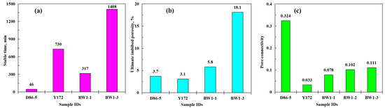
Figure 11.
The distribution of three parameters: (a) stable time, (b) ultimate imbibed porosity, and (c) pore connectivity.
4. Conclusions
This study aimed to bring out a quick method to investigate the pore connectivity and ultimate imbibed porosity of shale, leading to the following conclusions:
- (1)
- A quick method was established to measure the pore connectivity and ultimate imbibed porosity of shale by using spontaneous imbibition with thin samples. Within the time of a day, the imbibition results of 400 μm samples can be acquired.
- (2)
- The three parameters change with sample thicknesses. For sample D86-5, the average pore connectivity is 0.265 and the penetration depth is large, so water enters all connected pores, resulting in a stable ultimate imbibed porosity of around 3.7%. And the stable time increases with the addition of thicknesses. For sample Y172, when the thickness increases, the average pore connectivity is 0.026 and the penetration depth is much smaller with inaccessible pores, so the ultimate imbibed porosity declines with increasing thickness from 3.1% to 0.8%. The stable time of Y172 increases with the thickness from 460 μm to 680 μm before fluctuating around 1211 min, so the penetration depth of Y172 is between 230 μm and 340 μm.
- (3)
- Comparing the samples around 400 μm, the sample from the Qingshankou Fm has the smallest stable time and the largest pore connectivity, but the ultimate imbibed porosity is only 3.7%. The sample from the Shahejie Fm has a longer stable time and the smallest ultimate imbibed porosity and pore connectivity. The samples from the Liushagang Fm have the longest stable time and ultimate imbibed porosity and an average pore connectivity of 0.097.
For further research on pore connectivity and ultimate imbibed porosity with our method, different imbibition fluids and samples are suggested. In this study, we only used deionized water as the imbibition fluid, which can only appraise water-wet pores. Oil-wet fluid can investigate oil-wet pores, and amphiphilic fluid can examine mixed-wet pores. Simultaneously, fracturing fluid and formation water are also suggested. We only used shale as tested samples, and more samples are suggested, such as tight sandstone, carbonate, clastic volcanic rock, and so on. Furthermore, more pore structure characterizations should be conducted, such as nitrogen adsorption (NA), mercury intrusion porosimetry (MIP), nuclear magnetic resonance (NMR), and so on, which could help to analyze the controlling factors of pore connectivity and ultimate imbibed porosity.
Author Contributions
Conceptualization, Z.H. and M.M.; formal analysis, Z.H., M.M., K.D., J.B., Q.W., and X.L.; investigation, Z.H.; resources, M.M.; writing—original draft, Z.H.; writing—review and editing, M.M., K.D., J.B., Q.W., and X.L. All authors have read and agreed to the published version of the manuscript.
Funding
This research was funded by the National Natural Science Foundation of China (Grant Nos. 42372167 and 42102160), the “CUG Scholar” Scientific Research Funds at China University of Geosciences (Wuhan) (Project No.2022077), and the Fundamental Research Funds for the Central Universities, China University of Geosciences (Wuhan) (No. CUG240632).
Data Availability Statement
The data is contained within the article.
Conflicts of Interest
Author Xingchen Liu was employed by the company Cementing Company of Zhongyuan Petroleum Engineering Co., Ltd. under China Petrochemical Company Limited. The remaining authors declare that the research was conducted in the absence of any commercial or financial relationships that could be construed as a potential conflict of interest.
References
- Marchionna, M. Fossil energy: From conventional oil and gas to the shale revolution. EPJ Web Conf. 2018, 189, 00004. [Google Scholar] [CrossRef][Green Version]
- National Energy Administration. China’s Oil and Gas Industry Analysis and Outlook Series Blue Book. 2024. Available online: http://www.nea.gov.cn/2024-04/26/c_1310772762.htm (accessed on 26 April 2024).
- Loucks, R.; Reed, R.; Ruppel, S.; Hammes, U. Spectrum of pore types and networks in mudrocks and a descriptive classification for matrix related pores. AAPG Bull. 2012, 96, 1071–1098. [Google Scholar] [CrossRef]
- Chen, Y.; Jiang, C.; Leung, J.Y.; Wojtanowicz, A.K.; Zhang, D. Multiscale characterization of shale pore-fracture system: Geological controls on gas transport and pore size classification in shale reservoirs. J. Pet. Sci. Eng. 2021, 202, 108442. [Google Scholar] [CrossRef]
- Zhang, P.F.; Lu, S.F.; Li, J.Q.; Chang, X.C.; Zhang, J.J.; Pang, Y.M.; Lin, Z.Z.; Chen, G.; Yin, Y.J.; Liu, Y.Q. Quantitative characterization of shale pore connectivity and controlling factors using spontaneous imbibition combined with nuclear magnetic resonance T2 and T1-T2. Pet. Sci. 2023, 20, 1947–1960. [Google Scholar] [CrossRef]
- Ji, W.; Hao, F.; Gong, F.; Zhang, J.; Bai, Y.; Liang, C.; Tian, J. Petroleum migration and accumulation in a shale oil system of the Upper Cretaceous Qingshankou Formation in the Songliao Basin, northeastern China. AAPG Bull. 2024, 108, 1611–1648. [Google Scholar] [CrossRef]
- Jia, C.; Xiao, B.; Lijun, Y.; Yang, Z.; Yili, K. Experimental study of water imbibition characteristics of the lacustrine shale in Sichuan Basin. Petroleum 2023, 9, 572–578. [Google Scholar] [CrossRef]
- Wei, J.; Zhang, A.; Jiangtao, L.; Demiao, S.; Xiaofeng, Z. Study on microscale pore structure and bedding fracture characteristics of shale oil reservoir. Energy 2023, 278, 127829. [Google Scholar] [CrossRef]
- Yuan, Y.; Rezaee, R.; Mei-Fu, Z.; Stefan, I. A comprehensive review on shale studies with emphasis on nuclear magnetic resonance (NMR) technique. Gas Sci. Eng. 2023, 120, 205163. [Google Scholar] [CrossRef]
- Wang, Y.; Wang, Z.; Zhengchen, Z.; Shanshan, Y.; Hong, Z.; Guoqing, Z.; Feifei, L.; Lele, F.; Kouqi, L.; Liangliang, J. Recent techniques on analyses and characterizations of shale gas and oil reservoir. Energy Rev. 2024, 3, 100067. [Google Scholar] [CrossRef]
- Zhang, J.; Xiao, X.; Jianguo, W.; Wei, L.; Denglin, H.; Chenchen, W.; Yu, L.; Yan, X.; Xiaochan, Z. Pore structure and fractal characteristics of coal-bearing Cretaceous Nenjiang shales from Songliao Basin, Northeast China. J. Nat. Gas. Geosci. 2024, 9, 197–208. [Google Scholar] [CrossRef]
- Yasin, Q.; Liu, B.; Mengdi, S.; Ghulam Mohyuddin, S.; Atif, I.; Mariusz, M.; Naser, G.; Yan, M.; Xiaofei, F. Automatic pore structure analysis in organic-rich shale using FIB-SEM and attention U-Net. Fuel 2024, 358, 130161. [Google Scholar] [CrossRef]
- Norman, R.M.; Geoffrey, M. Recovery of oil by spontaneous imbibition. Curr. Opin. Colloid. Interface Sci. 2001, 6, 321–337. [Google Scholar] [CrossRef]
- Ding, Y.; Liu, X.; Liang, L.; Xiong, J.; Hou, L. Experimental and model analysis on shale spontaneous imbibition and its influence factors. J. Nat. Gas Sci. Eng. 2022, 99, 104462. [Google Scholar] [CrossRef]
- Meng, M.; Ge, H.; Yinghao, S.; Qinhong, H.; Longlong, L.; Zhiye, G.; Tonghui, T.; Jing, C. The effect of clay-swelling induced cracks on imbibition behavior of marine shale reservoirs. J. Nat. Gas. Sci. Eng. 2020, 83, 103525. [Google Scholar] [CrossRef]
- Meng, M.; Ge, H.; Yinghao, S.; Fei, R.; Wenming, J. A novel method for monitoring the imbibition behavior of clay-rich shale. Energy Rep. 2020, 6, 1811–1818. [Google Scholar] [CrossRef]
- Hu, J.; Zhao, H.; Du, X.; Zhang, Y. An analytical model for shut-in time optimization after hydraulic fracturing in shale oil reservoirs with imbibition experiments. J. Pet. Sci. Eng. 2022, 210, 110055. [Google Scholar] [CrossRef]
- Lan, Q.; Xu, M.; Binazadeh, M.; Dehghanpour, H.; Wood, J.M. A comparative investigation of shale wettability: The significance of pore connectivity. J. Nat. Gas Sci. Eng. 2015, 27, 1174–1188. [Google Scholar] [CrossRef]
- Vasheghani Farahani, M.; Mousavi Nezhad, M. On the effect of flow regime and pore structure on the flow signatures in porous media. Phys. Fluids 2022, 34, 115139. [Google Scholar] [CrossRef]
- Cheng, Z.; Tong, S.; Shang, X.; Yu, J.; Li, X.; Dou, L. Lattice Boltzmann simulation of counter-current imbibition of oil and water in porous media at the equivalent capillarity. AIP Adv. 2024, 14, 085314. [Google Scholar] [CrossRef]
- Alvarado, V.; Manrique, E. Chapter 2—Enhanced Oil Recovery Concepts. In Enhanced Oil Recovery; Alvarado, V., Manrique, E., Eds.; Gulf Professional Publishing: Boston, MA, USA, 2010; pp. 7–16. [Google Scholar]
- Yuan, S.; Han, H.; Wang, H.; Luo, J.; Wang, Q.; Lei, Z.; Xi, C.; Li, J. Research progress and potential of new enhanced oil recovery methods in oilfield development. Pet. Explor. Dev. 2024, 51, 963–980. [Google Scholar] [CrossRef]
- Valluri, S.; Claremboux, V.; Kawatra, S. Opportunities and challenges in CO2 utilization. J. Environ. Sci. 2022, 113, 322–344. [Google Scholar] [CrossRef] [PubMed]
- Cheng, Z.; Ning, Z.; Yu, X.; Wang, Q.; Zhang, W. New insights into spontaneous imbibition in tight oil sandstones with NMR. J. Pet. Sci. Eng. 2019, 179, 455–464. [Google Scholar] [CrossRef]
- Hamid, S.; Syed Mohammad, M.; Reza, R.; Ali, S. Conventional methods for wettability determination of shales: A comprehensive review of challenges, lessons learned, and way forward. Mar. Pet. Geol. 2021, 133, 105288. [Google Scholar] [CrossRef]
- Lin, Z.; Hu, Q.; Na, Y.; Shengyu, Y.; Huimin, L.; Jing, C. Nanopores-to-microfractures flow mechanism and remaining distribution of shale oil during dynamic water spontaneous imbibition studied by NMR. Geoenergy Sci. Eng. 2024, 241, 213202. [Google Scholar] [CrossRef]
- Wang, X.; Wang, M.; Li, Y.; Zhang, J.; Li, M.; Li, Z.; Guo, Z.; Li, J. Shale pore connectivity and influencing factors based on spontaneous imbibition combined with a nuclear magnetic resonance experiment. Mar. Pet. Geol. 2021, 132, 105239. [Google Scholar] [CrossRef]
- Liu, Z.; Bai, B.; Wang, Y.; Qu, H.; Xiao, Q.; Zeng, S. Spontaneous imbibition characteristics of slickwater and its components in Longmaxi shale. J. Pet. Sci. Eng. 2021, 202, 108599. [Google Scholar] [CrossRef]
- Liu, J.; Sheng, J.J. Experimental investigation of surfactant enhanced spontaneous imbibition in Chinese shale oil reservoirs using NMR tests. J. Ind. Eng. Chem. 2019, 72, 414–422. [Google Scholar] [CrossRef]
- Sun, M.; Yu, B.; Qinhong, H.; Rui, Y.; Yifan, Z.; Bo, L. Pore connectivity and tracer migration of typical shales in south China. Fuel 2017, 203, 32–46. [Google Scholar] [CrossRef]
- Lin, M.; Xi, K.; Cao, Y.; Liu, Q.; Zhang, Z.; Li, K. Petrographic features and diagenetic alteration in the shale strata of the Permian Lucaogou Formation, Jimusar sag, Junggar Basin. J. Pet. Sci. Eng. 2021, 203, 108684. [Google Scholar] [CrossRef]
- Wang, W.; Xie, Q.; Li, J.; Sheng, G.; Lun, Z. Fracturing fluid imbibition impact on gas-water two phase flow in shale fracture-matrix system. Nat. Gas Ind. B 2023, 10, 323–332. [Google Scholar] [CrossRef]
- Yang, R.; Hu, Q.; Yi, J.; Zhang, B.; He, S.; Guo, X.; Hou, Y.; Dong, T. The effects of mineral composition, TOC content and pore structure on spontaneous imbibition in Lower Jurassic Dongyuemiao shale reservoirs. Mar. Pet. Geol. 2019, 109, 268–278. [Google Scholar] [CrossRef]
- Yang, R.; Hu, Q.; Sheng, H.; Fang, H.; Xusheng, G.; Jizheng, Y.; Xipeng, H. Pore structure, wettability and tracer migration in four leading shale formations in the Middle Yangtze Platform, China. Mar. Pet. Geol. 2018, 89, 415–427. [Google Scholar] [CrossRef]
- Davudov, D.; Moghanloo, R.G.; Zhang, Y. Interplay between pore connectivity and permeability in shale sample. Int. J. Coal Geol. 2020, 220, 103427. [Google Scholar] [CrossRef]
- Yang, J.; Yang, B.; Liang, W.; Junliang, P.; Yunhui, F.; Yun, T. Invasion depths of fracturing fluid imbibition displacement in matrix pores of Da’an Zhai shale oil reservoirs in central Sichuan Basin. Pet. Geol. Recovery Effic. 2023, 30, 84–91. [Google Scholar]
- Ye, Y.; Tang, S.; Zhaodong, X.; Dexin, J.; Yang, D. Quartz types in the Wufeng-Longmaxi Formations in southern China: Implications for porosity evolution and shale brittleness. Mar. Pet. Geol. 2022, 137, 105479. [Google Scholar] [CrossRef]
- Tuzingila, R.M.; Kong, L.; Kasongo, R.K. A review on experimental techniques and their applications in the effects of mineral content on geomechanical properties of reservoir shale rock. Rock Mech. Bull. 2024, 3, 100110. [Google Scholar] [CrossRef]
- Xiao, D.; Zheng, L.; Jilin, X.; Min, W.; Rui, W.; Xiaodie, G.; Xueyi, G. Coupling control of organic and inorganic rock components on porosity and pore structure of lacustrine shale with medium maturity: A case study of the Qingshankou Formation in the southern Songliao Basin. Mar. Pet. Geol. 2024, 164, 106844. [Google Scholar] [CrossRef]
- Liu, B.; Mastalerz, M.; Schieber, J. SEM petrography of dispersed organic matter in black shales: A review. Earth-Sci. Rev. 2022, 224, 103874. [Google Scholar] [CrossRef]
- Wang, Q.; Li, Y.; Utley, J.E.P.; Gardner, J.; Liu, B.; Hu, J.; Shao, L.; Wang, X.; Gao, F.; Liu, D.; et al. Terrestrial dominance of organic carbon in an Early Cretaceous syn-rift lake and its correlation with depositional sequences and paleoclimate. Sediment. Geol. 2023, 455, 106472. [Google Scholar] [CrossRef]
- Meng, M.; Ge, H.; Shen, Y.; Ji, W. Evaluation of the Pore Structure Variation During Hydraulic Fracturing in Marine Shale Reservoirs. J. Energy Resour. Technol. 2020, 143, 083002. [Google Scholar] [CrossRef]
- Washburn, E.W. The Dynamics of Capillary Flow. Phys. Rev. 1921, 17, 273–283. [Google Scholar] [CrossRef]
- Handy, L.L. Determination of Effective Capillary Pressures for Porous Media from Imbibition Data. Trans. AIME 1960, 219, 75–80. [Google Scholar] [CrossRef]
- Hu, Q.; Ewing, R.P.; Dultz, S. Low pore connectivity in natural rock. J. Contam. Hydrol. 2012, 133, 76–83. [Google Scholar] [CrossRef] [PubMed]
- Zheng, Y.; Liao, Y.; Wang, J.; Xiong, Y.; Wang, Y.; Peng, P.a. Factors controlling the heterogeneity of shale pore structure and shale gas production of the Wufeng–Longmaxi shales in the Dingshan plunging anticline of the Sichuan Basin, China. Int. J. Coal Geol. 2024, 282, 104434. [Google Scholar] [CrossRef]
- Hao, L.; Qing, L.; Yue, D.; Wu, Y.; Gao, J.; Wu, S.; Wang, W.; Li, M.; An, K. Quantitative characterization and formation mechanism of the pore system heterogeneity: Examples from organic-rich laminated and organic-poor layered shales of the upper triassic chang 7 member in the southern Ordos Basin, China. Mar. Pet. Geol. 2023, 147, 105999. [Google Scholar] [CrossRef]
- Ge, H.-K.; Yang, L.; Shen, Y.-H.; Ren, K.; Meng, F.-B.; Ji, W.-M.; Wu, S. Experimental investigation of shale imbibition capacity and the factors influencing loss of hydraulic fracturing fluids. Pet. Sci. 2015, 12, 636–650. [Google Scholar] [CrossRef]


Disclaimer/Publisher’s Note: The statements, opinions and data contained in all publications are solely those of the individual author(s) and contributor(s) and not of MDPI and/or the editor(s). MDPI and/or the editor(s) disclaim responsibility for any injury to people or property resulting from any ideas, methods, instructions or products referred to in the content. |
© 2025 by the authors. Licensee MDPI, Basel, Switzerland. This article is an open access article distributed under the terms and conditions of the Creative Commons Attribution (CC BY) license (https://creativecommons.org/licenses/by/4.0/).