Ocean Currents Velocity Hindcast and Forecast Bias Correction Using a Deep-Learning Approach

 , , , and
Abstract
1. Introduction
2. Transform Model Concept
3. Methods
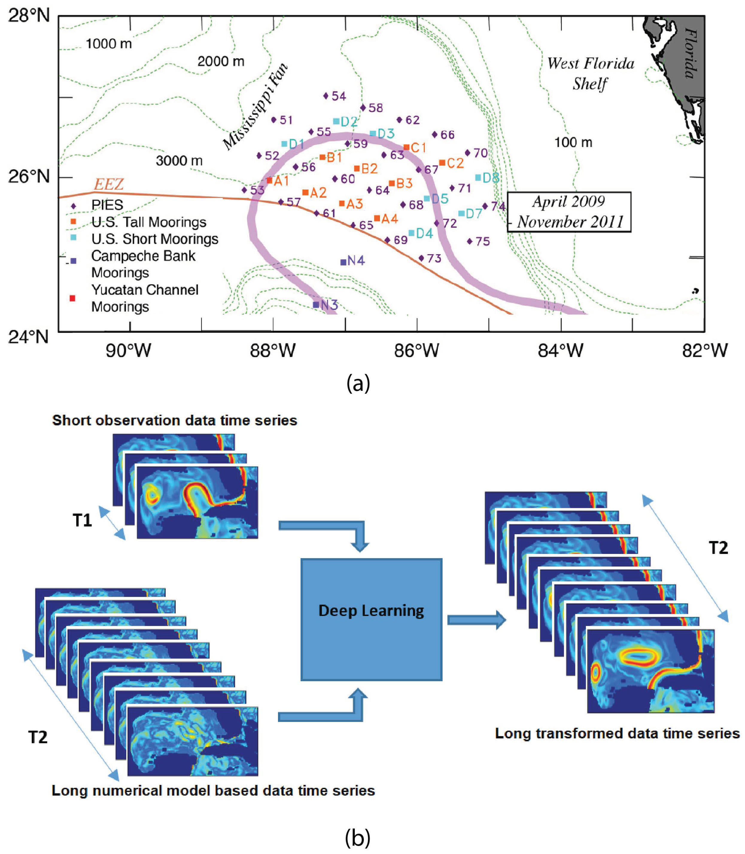
3.1. Data Sets
3.2. Transform Model
3.3. Experimental Strategy and Input Data Formatting
3.4. Bias Correction Evaluation Metrics
4. Results
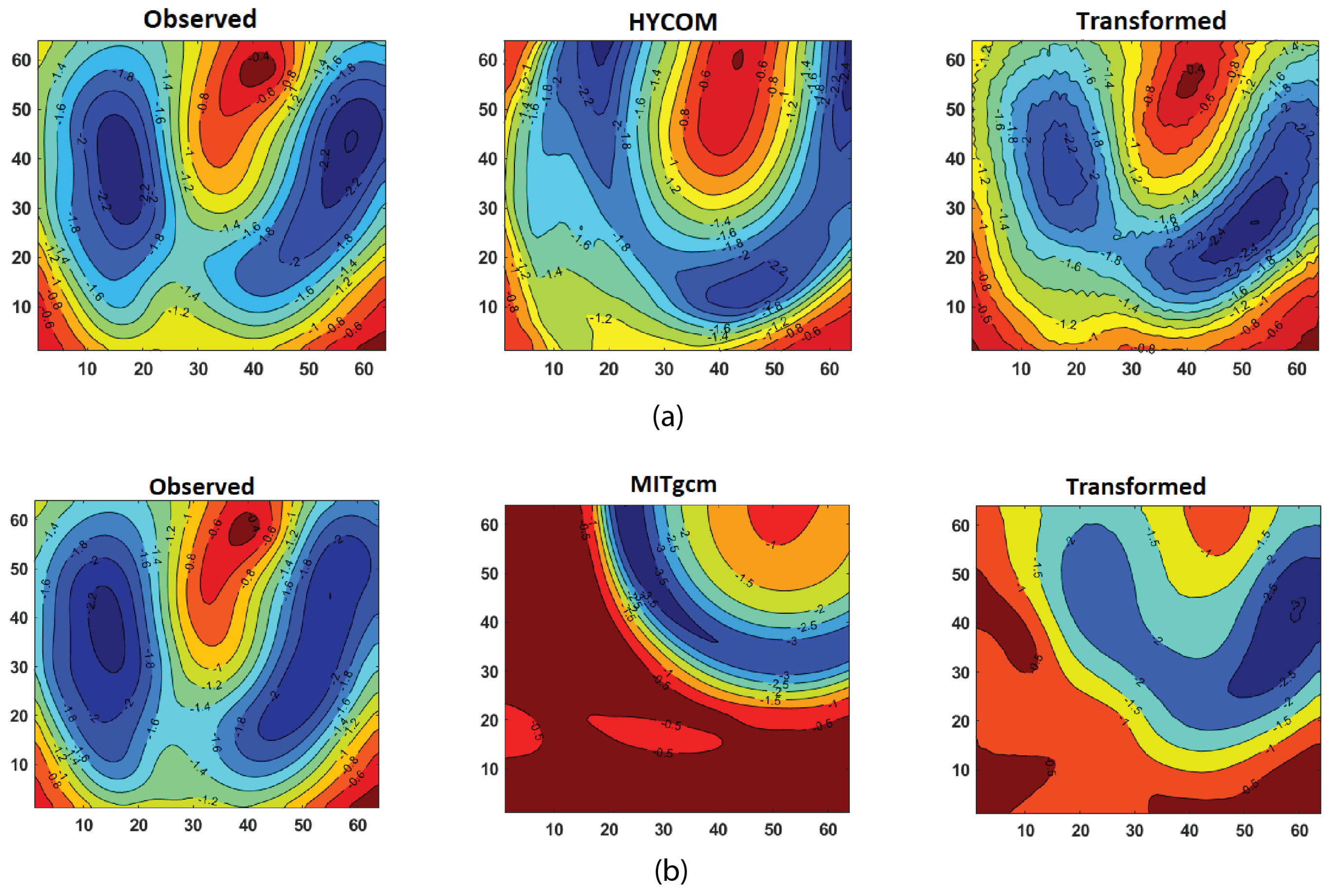
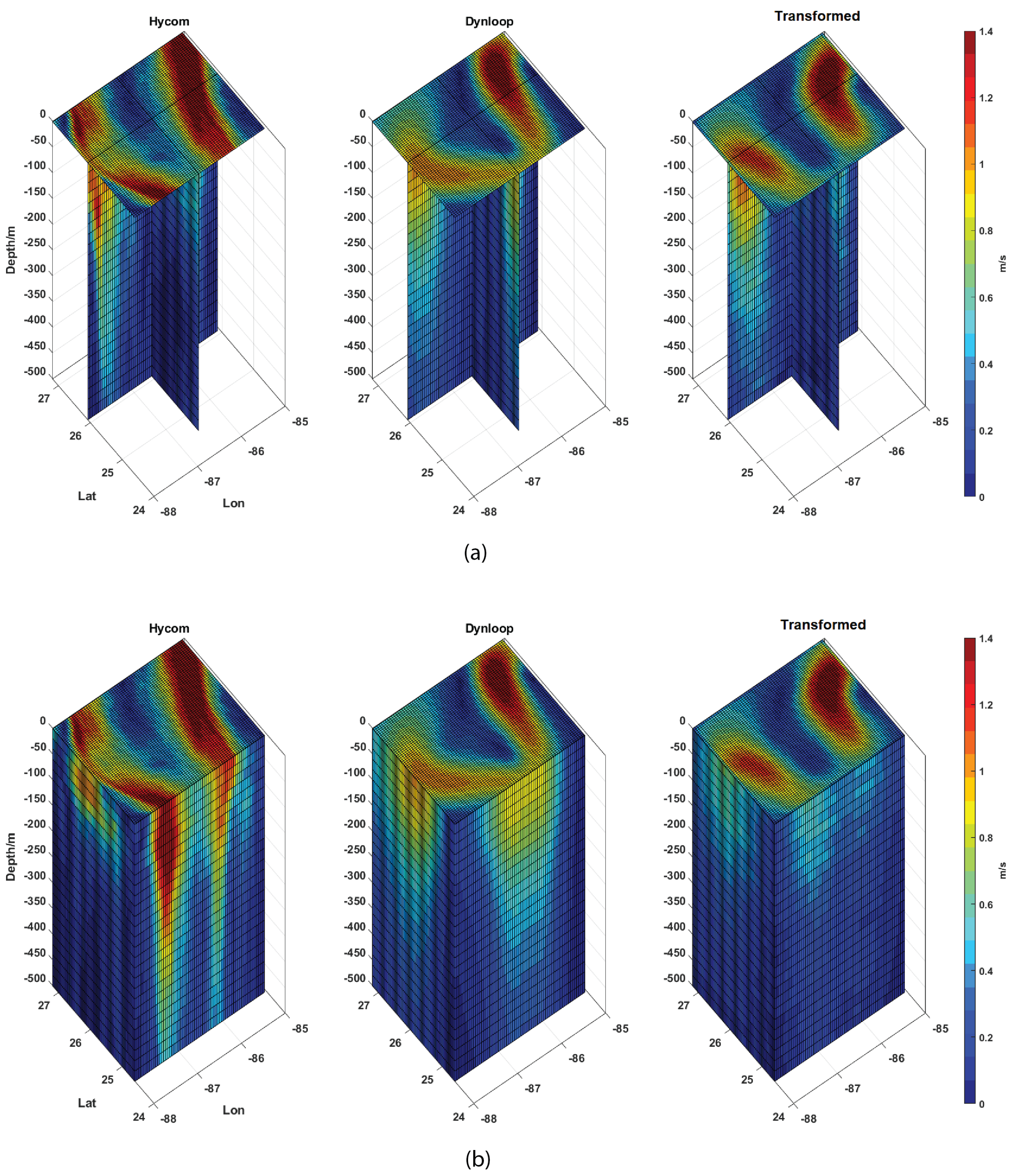
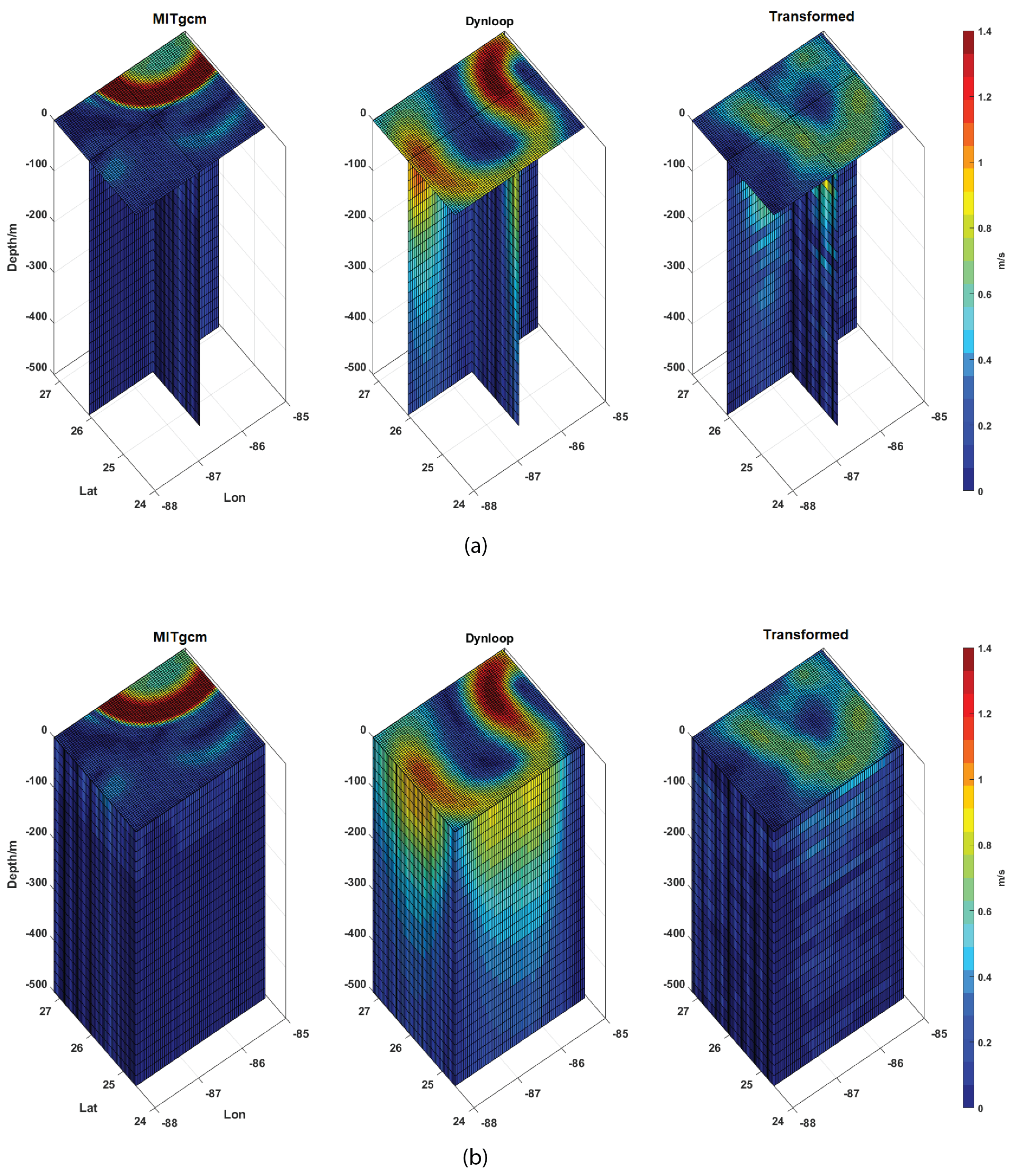
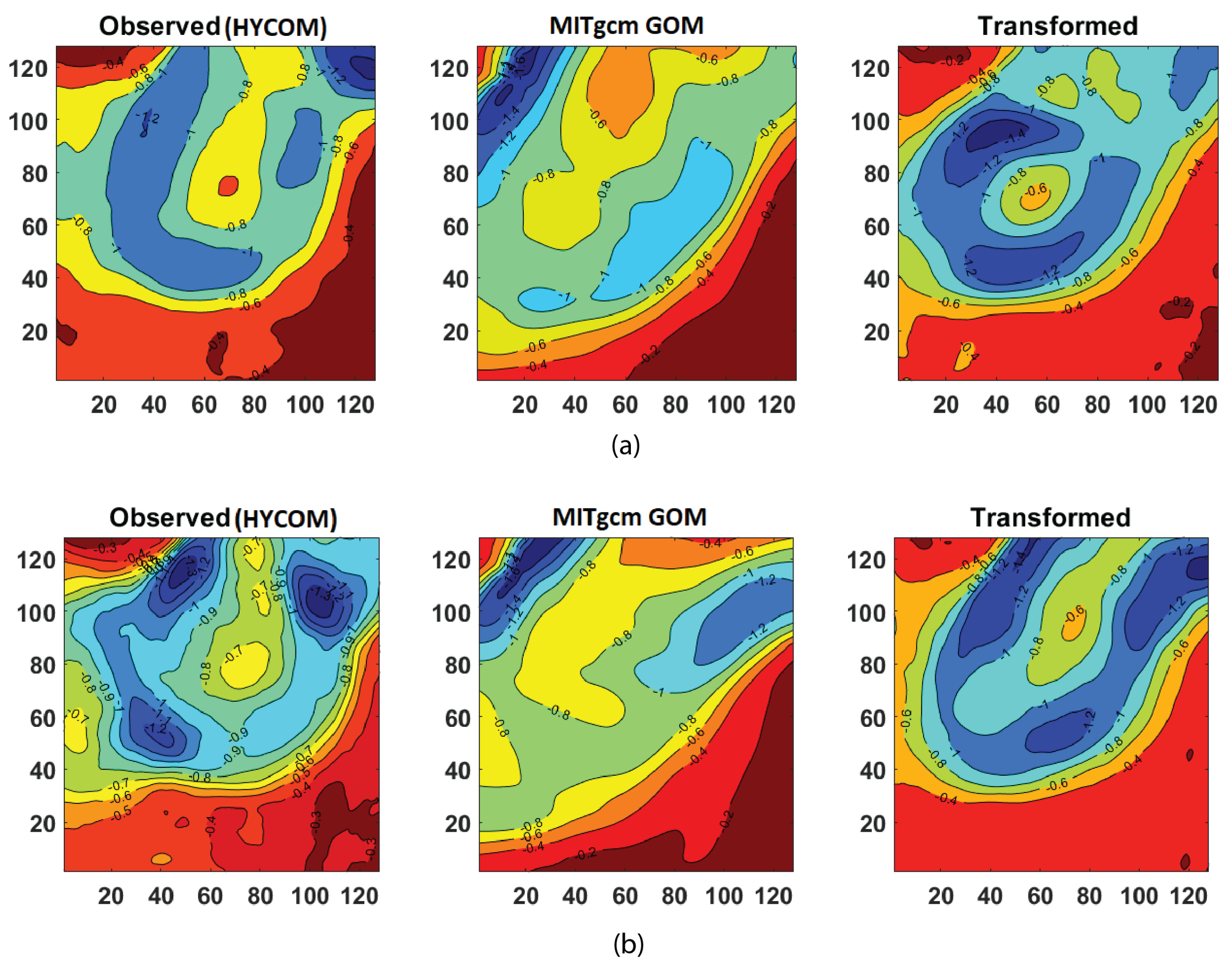
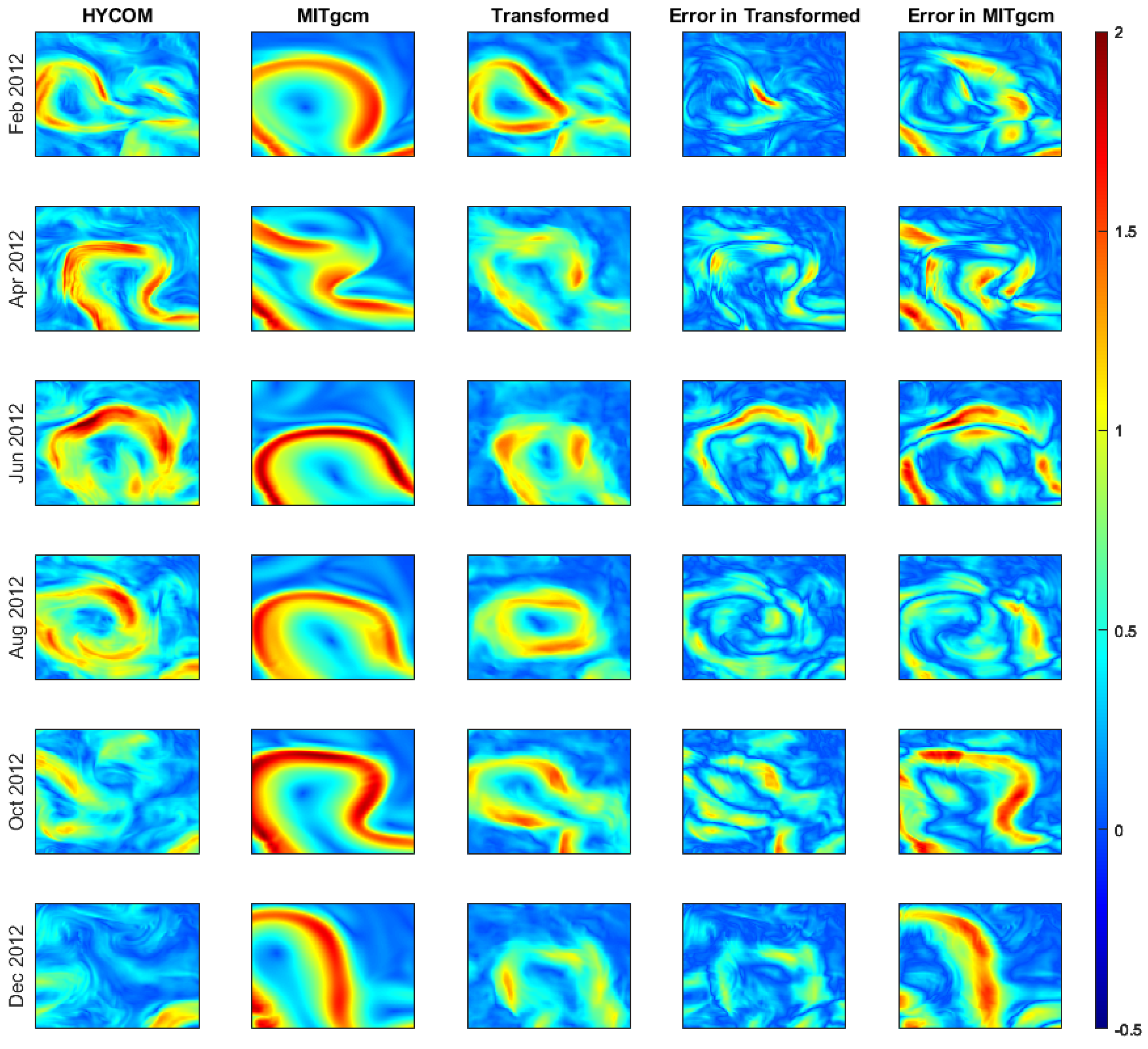
4.1. Comparison between Observed and Modeled Fields
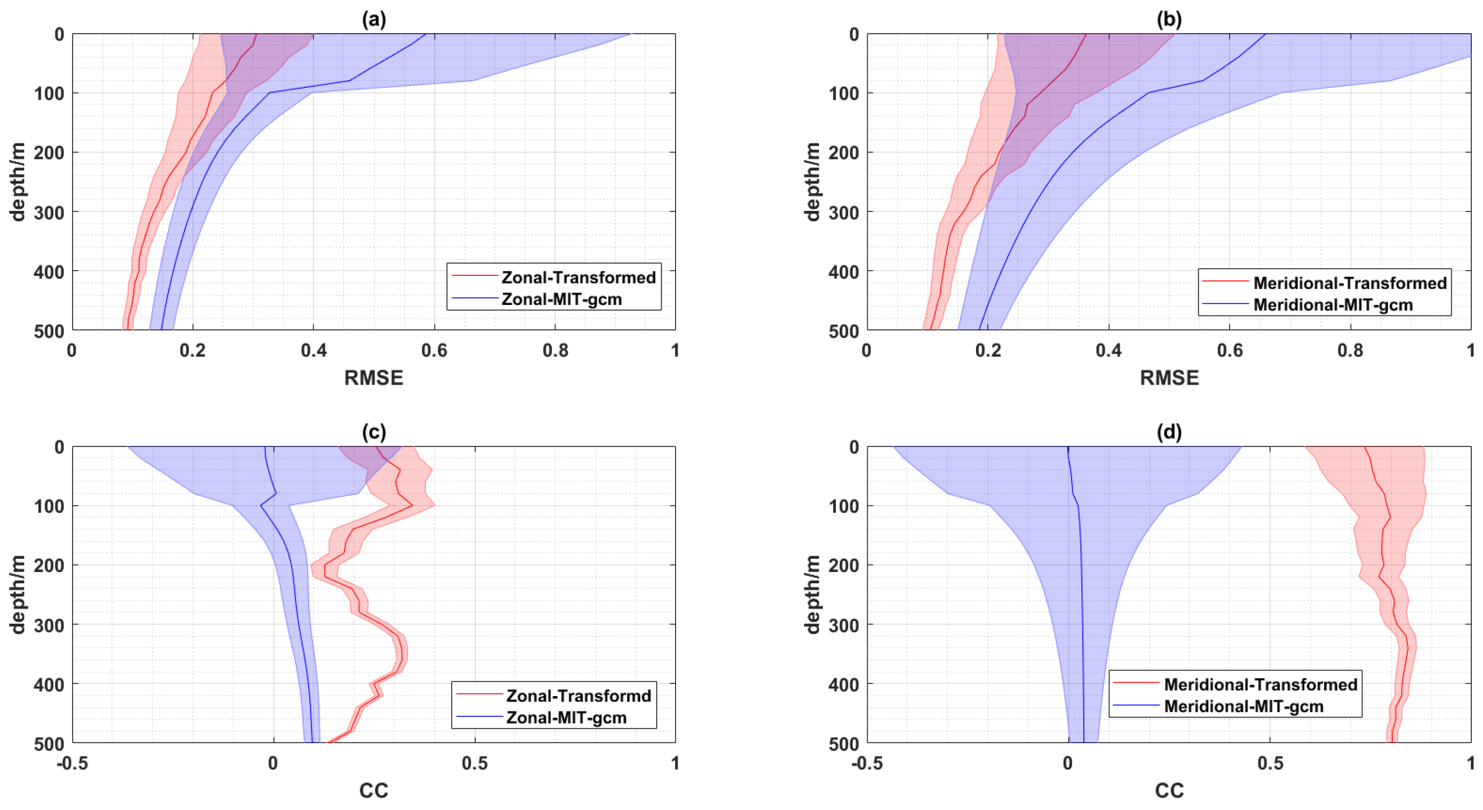
4.2. Evaluation of the Bias Correction by the Short-Term Transform Model
4.2.1. Two-Dimensional Field Bias Correction
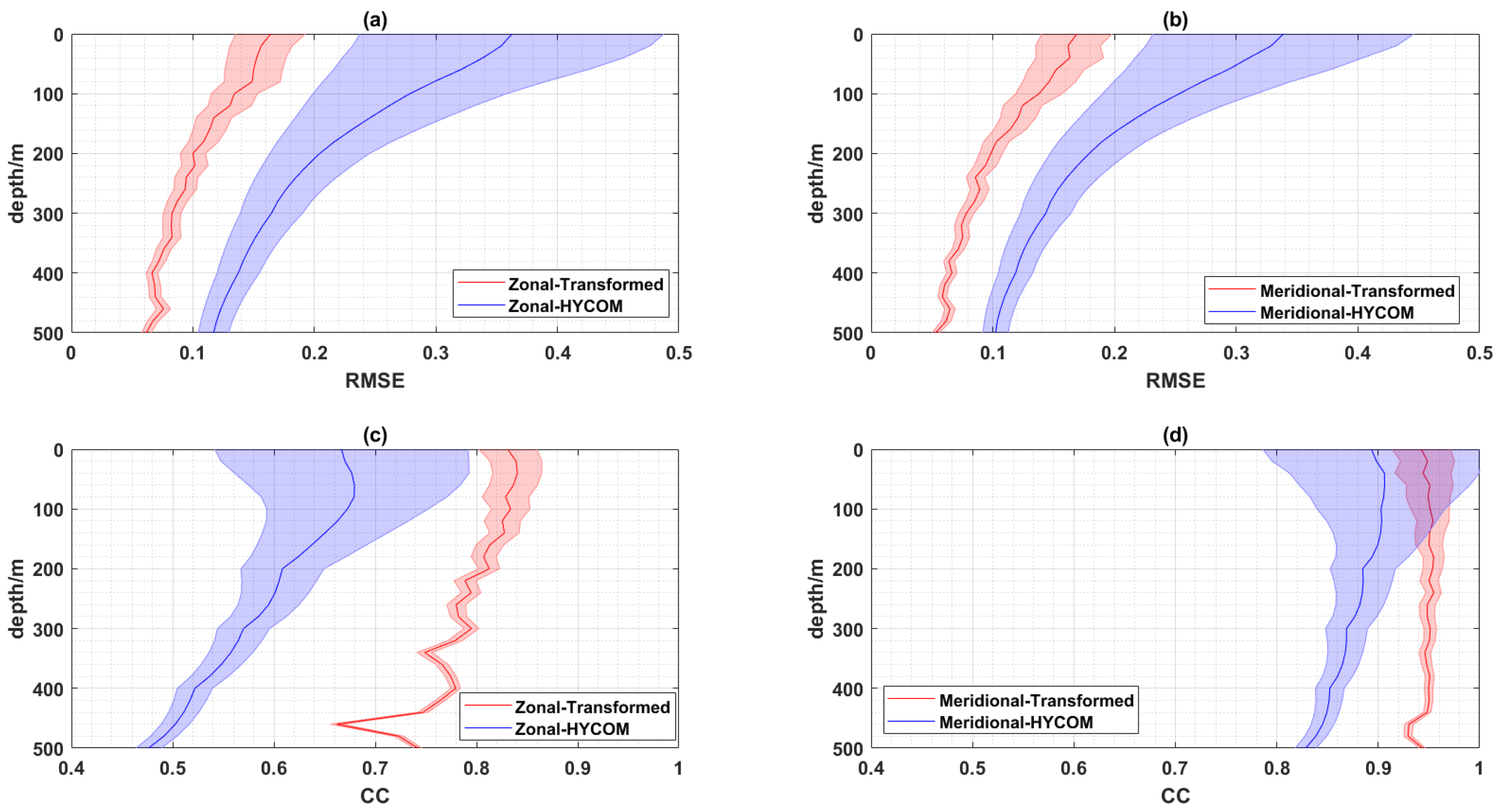
4.2.2. Three-Dimensional Field Bias Correction
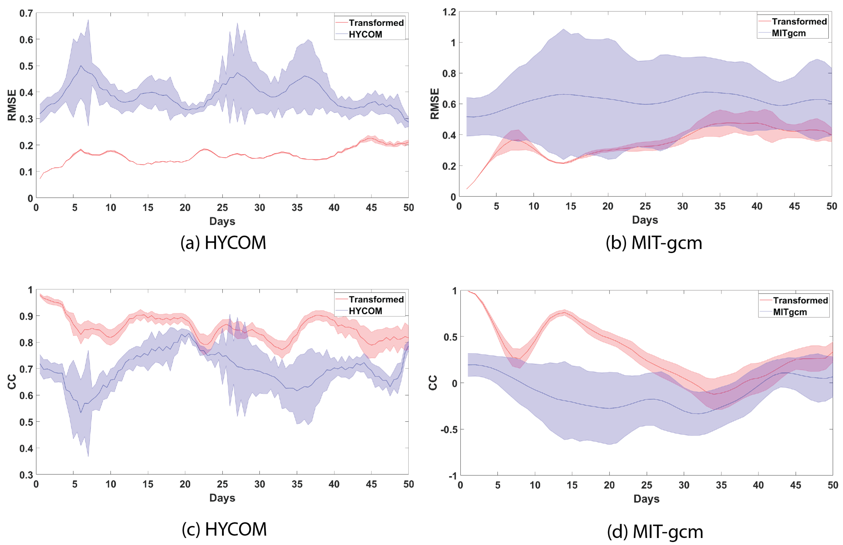
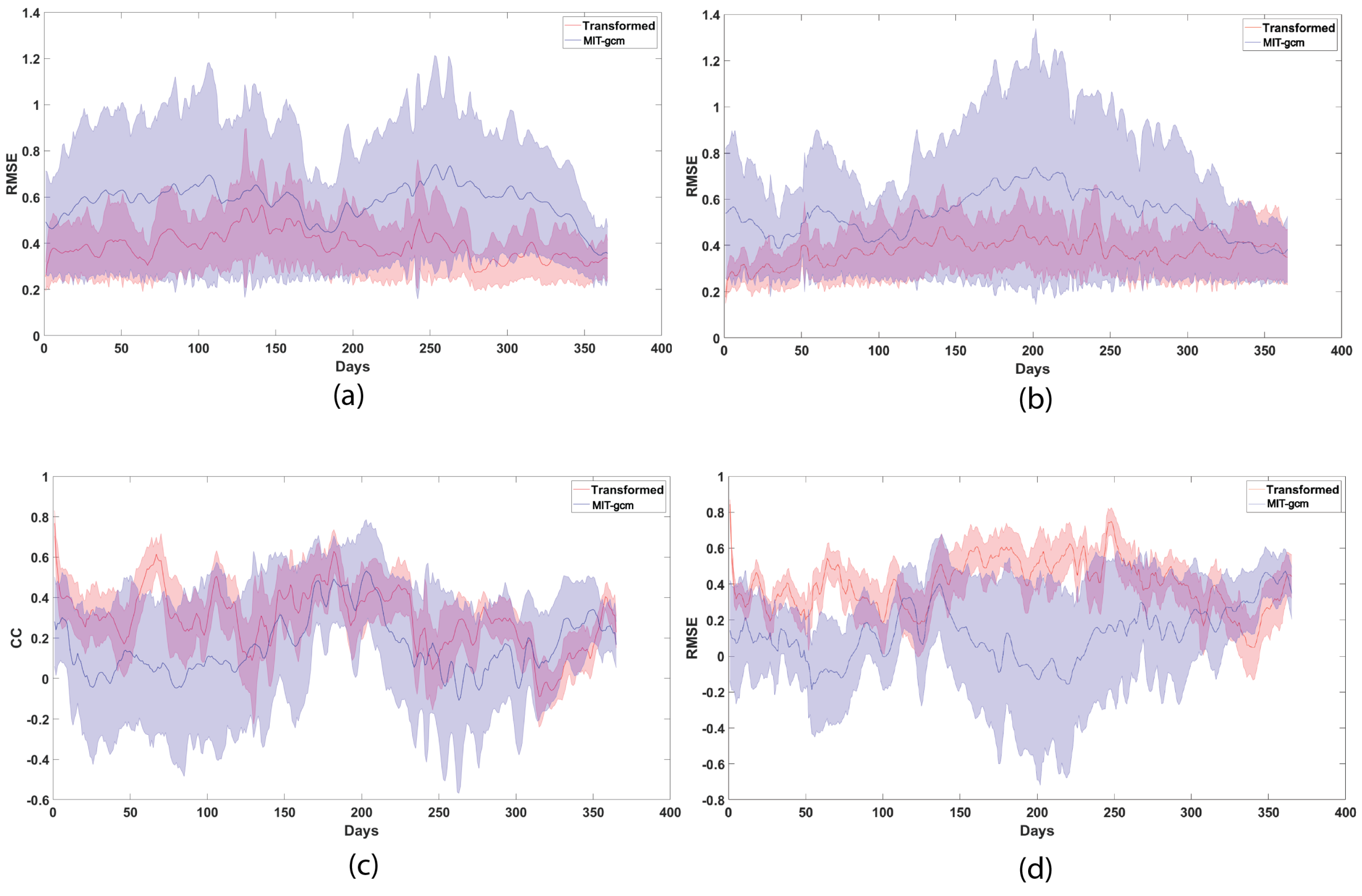
4.3. Evaluation of the Bias Correction by the Long-Term Transform Model
5. Conclusions
Author Contributions
Funding
Institutional Review Board Statement
Informed Consent Statement
Data Availability Statement
Acknowledgments
Conflicts of Interest
References
- Pozo Buil, M.; Fiechter, J.; Jacox, M.G.; Bograd, S.J.; Alexander, M.A. Evaluation of Different Bias Correction Methods for Dynamical Downscaled Future Projections of the California Current Upwelling System. Earth Space Sci. 2023, 10, e2023EA003121. [Google Scholar] [CrossRef]
- Vannitsem, S. Dynamical Properties of MOS Forecasts: Analysis of the ECMWF Operational Forecasting System. Weather Forecast. 2008, 23, 1032–1043. [Google Scholar] [CrossRef]
- Tian, D.; Martinez, C.J.; Graham, W.D.; Hwang, S. Statistical Downscaling Multimodel Forecasts for Seasonal Precipitation and Surface Temperature over the Southeastern United States. J. Clim. 2014, 27, 8384–8411. [Google Scholar] [CrossRef]
- Libonati, R.; Trigo, I.; DaCamara, C.C. Correction of 2 m-temperature forecasts using Kalman Filtering technique. Atmos. Res. 2008, 87, 183–197. [Google Scholar] [CrossRef]
- Pelosi, A.; Medina, H.; den Bergh, J.V.; Vannitsem, S.; Chirico, G.B. Adaptive Kalman Filtering for Postprocessing Ensemble Numerical Weather Predictions. Mon. Weather Rev. 2017, 145, 4837–4854. [Google Scholar] [CrossRef]
- Wang, J.; Chen, C.; Long, K.; Feng, L.; Research, M. Temporal and spatial distribution of short-time heavy rain of Sichuan Basin in summer. Plateau Mt. Meteorol. Res. 2015, 35, 16–20. [Google Scholar]
- Chepurin, G.A.; Carton, J.A.; Dee, D. Forecast Model Bias Correction in Ocean Data Assimilation. Mon. Weather Rev. 2005, 133, 1328–1342. [Google Scholar] [CrossRef]
- Mirouze, I.; Rémy, E.; Lellouche, J.M.; Martin, M.J.; Donlon, C.J. Impact of assimilating satellite surface velocity observations in the Mercator Ocean International analysis and forecasting global 1/4∘ system. Front. Mar. Sci. 2024, 11, 1376999. [Google Scholar] [CrossRef]
- Jäger, J.; Ferguson, H.L. Climate Change: Science, Impacts and Policy; Cambridge University Press: Cambridge, UK, 1991. [Google Scholar]
- Snowden, J.; Hernandez, D.; Quintrell, J.; Harper, A.; Morrison, R.; Morell, J.; Leonard, L. The U.S. Integrated Ocean Observing System: Governance Milestones and Lessons From Two Decades of Growth. Front. Mar. Sci. 2019, 6, 242. [Google Scholar] [CrossRef]
- Trice, A.; Robbins, C.; Philip, N.; Rumsey, M. Challenges and Opportunities for Ocean Data to Advance Conservation and Management; Ocean Conservancy: Washington, DC, USA, 2021. [Google Scholar]
- Boehme, L.; Rosso, I. Classifying Oceanographic Structures in the Amundsen Sea, Antarctica. Geophys. Res. Lett. 2021, 48, e2020GL089412. [Google Scholar] [CrossRef]
- Maze, G.; Mercier, H.; Fablet, R.; Tandeo, P.; Lopez Radcenco, M.; Lenca, P.; Feucher, C.; Le Goff, C. Coherent heat patterns revealed by unsupervised classification of Argo temperature profiles in the North Atlantic Ocean. Prog. Oceanogr. 2017, 151, 275–292. [Google Scholar] [CrossRef]
- Houghton, I.A.; Wilson, J.D. El Niño Detection Via Unsupervised Clustering of Argo Temperature Profiles. J. Geophys. Res. Ocean. 2020, 125, e2019JC015947. [Google Scholar] [CrossRef]
- Callaham, J.L.; Koch, J.V.; Brunton, B.W.; Kutz, J.N.; Brunton, S.L. Learning dominant physical processes with data-driven balance models. Nat. Commun. 2021, 12, 1016. [Google Scholar] [CrossRef] [PubMed]
- Pauthenet, E.; Roquet, F.; Madec, G.; Sallée, J.B.; Nerini, D. The Thermohaline Modes of the Global Ocean. J. Phys. Oceanogr. 2019, 49, 2535–2552. [Google Scholar] [CrossRef]
- Jones, D.C.; Holt, H.J.; Meijers, A.J.S.; Shuckburgh, E. Unsupervised Clustering of Southern Ocean Argo Float Temperature Profiles. J. Geophys. Res. Ocean. 2019, 124, 390–402. [Google Scholar] [CrossRef]
- Han, G.; Zhou, J.; Shao, Q.; Li, W.; Li, C.; Wu, X.; Cao, L.; Wu, H.; Li, Y.; Zhou, G. Bias correction of sea surface temperature retrospective forecasts in the South China Sea. Acta Oceanol. Sin. 2022, 41, 41–50. [Google Scholar] [CrossRef]
- Liu, G.; Bracco, A.; Brajard, J. Systematic Bias Correction in Ocean Mesoscale Forecasting Using Machine Learning. J. Adv. Model. Earth Syst. 2023, 15, e2022MS003426. [Google Scholar] [CrossRef]
- Yang, Z.; Liu, J.; Yang, C.Y.; Hu, Y. Correcting Nonstationary Sea Surface Temperature Bias in NCEP CFSv2 Using Ensemble-Based Neural Networks. J. Atmos. Ocean. Technol. 2023, 40, 885–896. [Google Scholar] [CrossRef]
- Choi, Y.; Park, Y.; Hwang, J.; Jeong, K.; Kim, E. Improving Ocean Forecasting Using Deep Learning and Numerical Model Integration. J. Mar. Sci. Eng. 2022, 10, 450. [Google Scholar] [CrossRef]
- Alvera-Azcárate, A.; Barth, A.; Weisberg, R.H. The Surface Circulation of the Caribbean Sea and the Gulf of Mexico as Inferred from Satellite Altimetry. J. Phys. Oceanogr. 2009, 39, 640–657. [Google Scholar] [CrossRef]
- Fei, T.; Huang, B.; Wang, X.; Zhu, J.; Chen, Y.; Wang, H.; Zhang, W. A Hybrid Deep Learning Model for the Bias Correction of SST Numerical Forecast Products Using Satellite Data. Remote Sens. 2022, 14, 1339. [Google Scholar] [CrossRef]
- Hamilton, P.; Lugo-Fernández, A.; Sheinbaum, J. A Loop Current experiment: Field and remote measurements. Dyn. Atmos. Ocean. 2016, 76, 156–173. [Google Scholar] [CrossRef]
- Walker, N. Coauthors, 2011: Impacts of Loop Current frontal cyclonic eddies and wind forcing on the 2010 Gulf of Mexico oil spill. Monitoring and Modeling the Deepwater Horizon Oil Spill: A Record-Breaking Enterprise. Geophys. Monogr. 2011, 195, 103–116. [Google Scholar]
- Jaimes, B.; Shay, L.K.; Brewster, J.K. Observed air-sea interactions in tropical cyclone Isaac over Loop Current mesoscale eddy features. Dyn. Atmos. Ocean. 2016, 76, 306–324. [Google Scholar] [CrossRef]
- Oey, L.Y.; Ezer, T.; Wang, D.P.; Fan, S.J.; Yin, X.Q. Loop current warming by Hurricane Wilma. Geophys. Res. Lett. 2006, 33, 1–4. [Google Scholar] [CrossRef]
- Kaiser, M.J.; Pulsipher, A.G. The potential value of improved ocean observation systems in the Gulf of Mexico. Mar. Policy 2004, 28, 469–489. [Google Scholar] [CrossRef]
- Wang, J.L.; Zhuang, H.; Chérubin, L.M.; Ibrahim, A.K.; Muhamed Ali, A. Medium-Term Forecasting of Loop Current eddy Cameron and eddy Darwin formation in the Gulf of Mexico with a Divide-and-Conquer Machine Learning Approach. J. Geophys. Res. Ocean. 2019, 124, 5586–5606. [Google Scholar] [CrossRef]
- Wang, J.L.; Zhuang, H.; Chérubin, L.; Muhamed Ali, A.; Ibrahim, A. Loop Current SSH Forecasting: A New Domain Partitioning Approach for a Machine Learning Model. Forecasting 2021, 3, 570–579. [Google Scholar] [CrossRef]
- Muhamed Ali, A.; Zhuang, H.; VanZwieten, J.; Ibrahim, A.K.; Chérubin, L. A Deep Learning Model for Forecasting Velocity Structures of the Loop Current System in the Gulf of Mexico. Forecasting 2021, 3, 934–953. [Google Scholar] [CrossRef]
- Huang, Y.; Tang, Y.; Zhuang, H.; VanZwieten, J.; Cherubin, L. Physics-Informed Tensor-Train ConvLSTM for Volumetric Velocity Forecasting of the Loop Current. Front. Artif. Intell. 2021, 4, 780271. [Google Scholar] [CrossRef]
- LeCun, Y.; Bengio, Y.; Hinton, G. Deep learning. Nature 2015, 521, 436–444. [Google Scholar] [CrossRef] [PubMed]
- Moore, A.M.; Martin, M.J.; Akella, S.; Arango, H.G.; Balmaseda, M.; Bertino, L.; Ciavatta, S.; Cornuelle, B.; Cummings, J.; Frolov, S.; et al. Synthesis of Ocean Observations Using Data Assimilation for Operational, Real-Time and Reanalysis Systems: A More Complete Picture of the State of the Ocean. Front. Mar. Sci. 2019, 6, 90. [Google Scholar] [CrossRef]
- Cooper, C.; Danmeier, D.; Frolov, S.; Stuart, G.; Zuckerman, S.; Anderson, S.; Sharma, N. Real Time Observing and Forecasting of Loop Currents in 2015. In Proceedings of the Offshore Technology Conference, Houston, TX, USA, 2–5 May 2016. [Google Scholar] [CrossRef]
- Cummings, J.A. Operational multivariate ocean data assimilation. Q. J. R. Meteorol. Soc. 2005, 131, 3583–3604. [Google Scholar] [CrossRef]
- Cummings, J.A.; Smedstad, O.M. Variational Data Assimilation for the Global Ocean; Springer: Berlin/Heidelberg, Germany, 2013; pp. 303–343. [Google Scholar]
- Fox, D.N.; Teague, W.J.; Barron, C.N.; Carnes, M.R.; Lee, C.M. The Modular Ocean Data Assimilation System (MODAS). J. Atmos. Ocean. Technol. 2002, 19, 240–252. [Google Scholar] [CrossRef]
- Saha, S.; Moorthi, S.; Pan, H.L.; Wu, X.; Wang, J.; Nadiga, S.; Tripp, P.; Kistler, R.; Woollen, J.; Behringer, D.; et al. The NCEP Climate Forecast System Reanalysis. Bull. Am. Meteorol. Soc. 2010, 91, 1015–1058. [Google Scholar] [CrossRef]
- Kalnay, E.; Kanamitsu, M.; Kistler, R.; Collins, W.; Deaven, D.; Gandin, L.; Iredell, M.; Saha, S.; White, G.; Woollen, J.; et al. The NCEP/NCAR 40-Year Reanalysis Project. Bull. Am. Meteorol. Soc. 1996, 77, 437–472. [Google Scholar] [CrossRef]
- Gopalakrishnan, G.; Cornuelle, B.D.; Hoteit, I. Adjoint sensitivity studies of loop current and eddy shedding in the Gulf of Mexico. J. Geophys. Res. Ocean. 2013, 118, 3315–3335. [Google Scholar] [CrossRef]
- Morey, S.L.; Gopalakrishnan, G.; Sanz, E.P.; de Souza, J.M.A.C.; Donohue, K.A.; Pérez-Brunius, P.; Dukhovskoy, D.S.; Chassignet, E.P.; Cornuelle, B.D.; Bower, A.S.; et al. Assessment of Numerical Simulations of Deep Circulation and Variability in the Gulf of Mexico Using Recent Observations. J. Phys. Oceanogr. 2020, 50, 1045–1064. [Google Scholar] [CrossRef]
- Donohue, K.; Watts, D.; Hamilton, P.; Leben, R.; Kennelly, M.; Lugo-Fernández, A. Gulf of Mexico loop current path variability. Dyn. Atmos. Ocean. 2016, 76, 174–194. [Google Scholar] [CrossRef]
- Donohue, K.; Watts, D.; Hamilton, P.; Leben, R.; Kennelly, M. Loop Current Eddy formation and baroclinic instability. Dyn. Atmos. Ocean. 2016, 76, 195–216. [Google Scholar] [CrossRef]
- Ronneberger, O.; Fischer, P.; Brox, T. U-net: Convolutional networks for biomedical image segmentation. In Proceedings of the International Conference on Medical Image Computing and Computer-Assisted Intervention, Munich, Germany, 5–9 October 2015; pp. 234–241. [Google Scholar]
- Siddique, N.; Sidike, P.; Elkin, C.; Devabhaktuni, V. U-Net and its variants for medical image segmentation: Theory and applications. arXiv 2020, arXiv:2011.01118. [Google Scholar] [CrossRef]
- Chacón, R.; Neila, P.; Salzmann, M.; Fua, P. A domain-adaptive two-stream U-net for electron microscopy image segmentation. In Proceedings of the 15th IEEE International Symposium Biomedical Imaging, number CONF, Washington, DC, USA, 4–7 April 2018. [Google Scholar]
- Li, R.; Liu, W.; Yang, L.; Sun, S.; Hu, W.; Zhang, F.; Li, W. Deepunet: A deep fully convolutional network for pixel-level sea-land segmentation. IEEE J. Sel. Top. Appl. Earth Obs. Remote Sens. 2018, 11, 3954–3962. [Google Scholar] [CrossRef]
- Jiao, L.; Huo, L.; Hu, C.; Tang, P. Refined unet: Unet-based refinement network for cloud and shadow precise segmentation. Remote Sens. 2020, 12, 2001. [Google Scholar] [CrossRef]
- Fernández, J.G.; Abdellaoui, I.A.; Mehrkanoon, S. Deep coastal sea elements forecasting using U-Net based models. arXiv 2020, arXiv:2011.03303. [Google Scholar]
- Dang, K.B.; Nguyen, M.H.; Nguyen, D.A.; Phan, T.T.H.; Giang, T.L.; Pham, H.H.; Nguyen, T.N.; Tran, T.T.V.; Bui, D.T. Coastal Wetland Classification with Deep U-Net Convolutional Networks and Sentinel-2 Imagery: A Case Study at the Tien Yen Estuary of Vietnam. Remote Sens. 2020, 12, 3270. [Google Scholar] [CrossRef]
- Shaikhina, T.; Khovanova, N.A. Handling limited datasets with neural networks in medical applications: A small-data approach. Artif. Intell. Med. 2017, 75, 51–63. [Google Scholar] [CrossRef]
- Keys, R. Cubic convolution interpolation for digital image processing. IEEE Trans. Acoust. Speech Signal Process. 1981, 29, 1153–1160. [Google Scholar] [CrossRef]
- Muhamed Ali, A.; Zhuang, H.; Ibrahim, A.K.; Wang, J.L.; Chérubin, L.M. Deep learning prediction of two-dimensional ocean dynamics with wavelet-compressed data. Front. Artif. Intell. 2022, 5, 923932. [Google Scholar] [CrossRef]
- Jolliff, J.K.; Kindle, J.C.; Shulman, I.; Penta, B.; Friedrichs, M.A.; Helber, R.; Arnone, R.A. Summary diagrams for coupled hydrodynamic-ecosystem model skill assessment. J. Mar. Syst. 2009, 76, 64–82. [Google Scholar] [CrossRef]
- Thomson, R.E.; Emery, W.J. Data Analysis Methods in Physical Oceanography, 3rd ed.; Elsevier Science: Amsterdam, The Netherlands, 2014. [Google Scholar] [CrossRef]
- Cooper, M.; Haines, K. Altimetric assimilation with water property conservation. J. Geophys. Res. 1996, 101, 1059–1077. [Google Scholar] [CrossRef]
- Chérubin, L.M.; Morel, Y.; Chassignet, E.P. Loop Current Ring Shedding: The Formation of Cyclones and the Effect of Topography. J. Phys. Oceanogr. 2006, 36, 569–591. [Google Scholar] [CrossRef]
- Chérubin, L.M.; Sturges, W.; Chassignet, E.P. Deep flow variability in the vicinity of the Yucatan Straits from a high-resolution numerical simulation. J. Geophys. Res. Ocean. 2005, 110, C04009. [Google Scholar] [CrossRef]
- Speich, S.; Rodrigues, R.R.; Santos, J.; Li, J. Special Issue “Tropical Atlantic Ocean Observing System”. Clivar Exch. 2022, 82, 156–173. [Google Scholar] [CrossRef]
- Mantovani, C.; Corgnati, L.; Horstmann, J.; Rubio, A.; Reyes, E.; Quentin, C.; Cosoli, S.; Asensio, J.L.; Mader, J.; Griffa, A. Best Practices on High Frequency Radar Deployment and Operation for Ocean Current Measurement. Front. Mar. Sci. 2020, 7, 210. [Google Scholar] [CrossRef]
- Fringer, O.B.; Dawson, C.N.; He, R.; Ralston, D.K.; Zhang, Y.J. The future of coastal and estuarine modeling: Findings from a workshop. Ocean Model 2019, 143, 101458. [Google Scholar] [CrossRef]


| Dataset | Zonal | Zonal | Zonal | Meridional | Meridional | Meridional |
|---|---|---|---|---|---|---|
| Depth | 0 m | 100 m | 500 m | 0 m | 100 m | 500 m |
| HYCOM | ||||||
| MITgcm |
Disclaimer/Publisher’s Note: The statements, opinions and data contained in all publications are solely those of the individual author(s) and contributor(s) and not of MDPI and/or the editor(s). MDPI and/or the editor(s) disclaim responsibility for any injury to people or property resulting from any ideas, methods, instructions or products referred to in the content. |
© 2024 by the authors. Licensee MDPI, Basel, Switzerland. This article is an open access article distributed under the terms and conditions of the Creative Commons Attribution (CC BY) license (https://creativecommons.org/licenses/by/4.0/).
Share and Cite
Muhamed Ali, A.; Zhuang, H.; Huang, Y.; Ibrahim, A.K.; Altaher, A.S.; Chérubin, L.M. Ocean Currents Velocity Hindcast and Forecast Bias Correction Using a Deep-Learning Approach. J. Mar. Sci. Eng. 2024, 12, 1680. https://doi.org/10.3390/jmse12091680
Muhamed Ali A, Zhuang H, Huang Y, Ibrahim AK, Altaher AS, Chérubin LM. Ocean Currents Velocity Hindcast and Forecast Bias Correction Using a Deep-Learning Approach. Journal of Marine Science and Engineering. 2024; 12(9):1680. https://doi.org/10.3390/jmse12091680
Chicago/Turabian StyleMuhamed Ali, Ali, Hanqi Zhuang, Yu Huang, Ali K. Ibrahim, Ali Salem Altaher, and Laurent M. Chérubin. 2024. "Ocean Currents Velocity Hindcast and Forecast Bias Correction Using a Deep-Learning Approach" Journal of Marine Science and Engineering 12, no. 9: 1680. https://doi.org/10.3390/jmse12091680
APA StyleMuhamed Ali, A., Zhuang, H., Huang, Y., Ibrahim, A. K., Altaher, A. S., & Chérubin, L. M. (2024). Ocean Currents Velocity Hindcast and Forecast Bias Correction Using a Deep-Learning Approach. Journal of Marine Science and Engineering, 12(9), 1680. https://doi.org/10.3390/jmse12091680