Recognition and Prediction of Multi-Level Handling Complexity at Automated Terminals Based on ARIMA

Abstract

Accurate recognition and prediction of the multi-level handling complexity in automated container terminals (referred to as “automated terminals”) is a prerequisite for improving the effectiveness of scheduling and realizing intelligent operation and maintenance. According to the operating characteristics of the automated terminal equipment, the operating network is constructed of automated terminals that describe the characteristics of operating complexity. We use K-medoids and a light gradient boosting machine (LightGBM) to construct a K-LightGBM model that recognizes multi-level handling complexity. The key lies in the reasonable construction of prediction models. A hyper-heuristic autoregressive integrated moving average (ARIMA) model is proposed to address the problem that the ARIMA is ineffective in predicting nonlinear data. We combine ARIMA and the LightGBM model to establish an ARIMA-LightGBM model to predict multi-level handling and residuals. To improve accuracy, we propose the two residual prediction strategies of direct prediction and limited residual boundary prediction based on the residuals generated by ARIMA. We propose a hyper-heuristic algorithm based on a gradient descent-trust region (GD-TR) to compute the weights of predicted values under the two strategies, which improves the global search capability by GD and TR. The particle swarm optimization algorithm, simulated annealing algorithm, and ant colony optimization algorithm are low-level heuristics. Simulation results show that the proposed model possesses the lowest root mean square error on all characteristics compared to ARIMA, E-ARIMA, and ARIMA-LSTM. Therefore, the proposed model is very effective in improving the accuracy of predicting the multi-level handling complexity at automated terminals.

1. Introduction

An automated terminal realizes the automation of multi-level loading or unloading handling (multi-level handling for short). Multi-level handling includes quay crane (QC) loading or unloading, automated guided vehicle (AGV) horizontal transportation, and the yard crane (YC) loading or unloading of containers. Multi-level handling is a dynamic, discrete, and random multi-level logistics system [1].

Some researchers have focused on QC operation by assigning QC to arrive at berths on time and the sequence of loading and unloading containers [2,3]. Events about AGV path planning, such as conflicts and collisions, are a hot research topic for AGV operation [4,5]. Several researchers on YC operation have focused on efficiency and energy consumption [6,7]. However, the complexity of multi-level operations has generally been overlooked when exploring scheduling schemes for multi-level operations in automated terminals. This is likely to result in the formulation of scheduling strategies that are not adequately adapted to the actual operational scenarios, which in turn adversely affects the overall operational efficiency of the terminal. In contrast, research on the complexity of transportation is relatively well established. Sharma et al. [8] and Sui et al. [9] reduced the collision risk of marine vessels through their operational posture. Automated terminals have complex operations, weak data regularity in multi-level logistics operations, and stochastic dynamic systems that are highly susceptible to uncertainties. In order to accurately grasp operational trends and improve scheduling effectiveness, there is an urgent need to accurately predict their handling complexity.

The key to realizing automated terminal handling complexity prediction lies in the construction of prediction models. How to improve the prediction performance of the models is still a challenging problem at this stage. Currently, prediction models are mainly categorized into parametric, nonparametric, and hybrid models.

Autoregressive integrated moving average (ARIMA) is a commonly used parametric model with a simple structure. ARIMA does not require external parameters to build forecasts, and has a huge advantage in the regression of linear data. However, when facing large-scale nonlinear data such as multi-level logistics operational data, the model often fails to achieve satisfactory prediction results [10]. Nonparametric models are usually based on machine learning, including random forest [11], support vector machines [12], and artificial neural networks [13,14], which have a better fitting effect on nonlinear data. However, nonparametric models have poor interpretability and long training times. Based on parametric and nonparametric models, many scholars have proposed hybrid models to improve the prediction effect on large-scale nonlinear data. Shahriari et al. [15] combined the self-service sampling method with the traditional parametric ARIMA model and proposed the E-ARIMA model that integrates multiple ARIMA models. The prediction accuracy of the E-ARIMA model is mainly determined by ARIMA, and if the experimental data do not meet the premise assumptions or applicability conditions of the ARIMA model, the prediction accuracy of the E-ARIMA model will definitely be negatively affected. Lu et al. [16] firstly used rolling regression ARIMA model to capture linear regression features, and then used back propagation on LSTM network to capture nonlinear features. They weighted the predicted values of the two models based on sliding window as the final result. However, model parameter tuning is difficult and requires massive historical data.

This paper constructs a complex network model based on multi-level logistics operations in automated terminals, and uses its topological features to accurately describe the complexity of the operation process. Complex networks [17] have been widely used in many fields, including transportation networks [18,19], epidemics [20,21], and other fields. In the research related to automated terminals, Li et al. [1] proposed a two-layer dynamic risk propagation and evolution model based on complex networks. They analyzed the adverse impacts of risk propagation and evolution, thus verifying the feasibility of applying the theory related to complex networks in the field of automated terminals. Complexity theory is applied to construct an automated terminal operation network using operational equipment as nodes and operational interactions between equipment as edges. Based on this network, the handling complexity is described using its corresponding topological features, which in turn are used as features of the prediction model. We construct the K-LightGBM model as the recognition model to capture the trend of multi-level handling. To improve the prediction accuracy, a hybrid ARIMA-LightGBM prediction model is proposed, in which ARIMA [22] is used for initial prediction and a light gradient boosting machine [23] (LightGBM) focuses on predicting the residuals generated by ARIMA. In order to deal with the residual data in a more detailed way, two strategies are designed. One strategy is to directly input the residual dataset into the ARIMA-LightGBM model for prediction. The other strategy is to set the maximum and minimum values of the residual data. When the data exceeds the maximum and minimum values, it is replaced by set maximum and minimum values. To fully utilize the advantages of both strategies, appropriate weights are further assigned to these two residual prediction strategies. Considering that the traditional gradient descent method [24] (GD) easily falls into local optimal solutions during the solution process, a hyper-heuristic algorithm based on a gradient descent-trust region (GD-TR) is proposed for assigning weights by combining it with the TR algorithm [25]. The algorithm is able to obtain a trust domain interval containing the global optimal solution during the search process, which leads to the global optimal weight assignment. Through comparative tests, the proposed model is proven to be very effective in improving the accuracy of automated terminal handling complexity predictions.

The rest of the paper is organized as follows. Section 2 introduces the method of complex networks for multi-level handling at automated terminals. Section 3 describes the complexity of multi-level handling and designs the recognition model. Section 4 creates the prediction model of multi-level handling at automated terminals, proposes two residual prediction strategies, and designs a hyper-heuristic algorithmic architecture to compute the weights of two residual prediction strategies. Section 5 presents and discusses the test results of the proposed methodology. Conclusions are provided in Section 6.

2. Handling Network at Automated Terminal

2.1. Automated Terminal Operation Network Construction

The automated terminal handling network consists of the QC handling network and the YC handling network. The nodes of the QC handling network are QCs and AGVs. In a certain time period, a QC may have operational task connections with multiple AGVs, and there may be path conflicts and mutual waiting between AGVs. There are edge connections between QCs and the corresponding AGVs, and there are edge connections between AGVs operating under the same QC. In contrast, QCs cannot be crossed at will due to physical location constraints, so there are edge connections between QCs, but they cannot form a closed loop. Similarly, the nodes of the YC handling network are YCs and AGVs. There are edge connections between YCs and corresponding AGVs, edge connections between AGVs operating under the same YC, and edge connections between YCs between the same yards.

In the QC/YC handling network, multiple AGVs have operational interactions with the same QC/YC, which is in line with the characteristics of tight connectivity or high correlation between community nodes [26,27]. Where QCs/YCs are community centers, an example of a specific automated terminal operation network is shown in Figure 1.

2.2. Analysis of the Handling Situation

Different numbers of AGVs, QCs, and YCs of multi-level handling will lead to a different complexity of handling situations. The following are several cases of different complexity. Condition 1: Figure 2a shows only one QC/YC is in handling, and only one AGV has loading or unloading tasks. Condition 2: Figure 2b shows only one QC/YC is handling, but two AGVs have loading or unloading tasks. Condition 3: Figure 2c shows two QCs/YCs are in handling. One QC/YC has loading or unloading tasks with two AGVs, and the other QC/YC has loading or unloading tasks with one AGV.

From the perspective of resource scheduling and complex networks, it can be seen that the complexity of these three cases increases sequentially. When the automated terminal is operated, QCs/YCs will have interactive tasks with multiple AGVs. It is more complex than these three cases.

3. The Handling Complexity at Automated Terminal

3.1. Description of the Handling Complexity at Automated Terminal

The handling complexity (hc) is defined using the number of nodes, average degree, network clustering coefficient, and number of communities as in Equation (1):

$$hc=(N,\stackrel{\rightharpoonup }{K},\stackrel{\rightharpoonup }{C},CM)$$

(1)

(1)

Number of nodes: N

The node number is the total number of nodes in a complex network. This can reflect the total number of equipment units participating in the handling.

$$N=N_{QC}+N_{AGV}$$

(2)

$$N=N_{YC}+N_{AGV}$$

(3)

(2)

Average degree: $\stackrel{\rightharpoonup }{K}$

The degree of a node is the number of connected edges of the node. This means the number of direct neighbors. The average degree is calculated by summing up the degrees of all nodes within the network and then dividing this sum by the total number of nodes.

The average degree can reflect the number of AGVs handling in the same QC/YC handling area. The average degree of the network, $\stackrel{\rightharpoonup }{K}$, is shown in Equation (4):

$$\stackrel{\rightharpoonup }{K}={\displaystyle \frac{1}{N}}{\displaystyle \sum _{i=1}^N{K}_i}$$

(4)

where K_i is the degree of the node i.

(3)

Average clustering coefficient: $\stackrel{\rightharpoonup }{C}$

The clustering coefficient reflects the clustering characteristics of the network. The average clustering coefficient can reflect the number of AGVs waiting in the QC/YC handling area. The higher the average clustering coefficient and the number of AGVs waiting, the higher the complexity of the entire network. The average clustering coefficient of the network, $\stackrel{\rightharpoonup }{C}$, is defined as follows:

$$c_i={\displaystyle \frac{1}{s_i(k_i-1)}}{\displaystyle \sum _{j,k\in N_i}\frac{w_{ij}+w_{ik}}{2}{a}_{ijk}}$$

(5)

$$\stackrel{\rightharpoonup }{C}={\displaystyle \frac{1}{N}}{\displaystyle \sum _{i=1}^N{c}_i}$$

(6)

$$a_{ijk}=\left\{\begin{array}{l}1 If i,j,k can form a closed triangle\\ 0 If i,j,k can’t form a closed triangle\end{array}\right.$$

(7)

where c_i is the clustering coefficient of the node i.

(4)

Number of communities: CM

Communities divide the nodes in the network into several “clusters”. The connections among nodes in the cluster are dense, and the node connections among different clusters are sparse.

Take an automated terminal with an annual throughput of about 6 million twenty-foot equivalent units (TEU) as an example. The loading or unloading time of a single container handled by QC is two minutes. The average hourly rate for the number of containers loaded and unloaded by QC can be 58.28 in multi-level handling. It can be seen that in twenty minutes, the amount of loading or unloading handled by a QC is about nine containers. Therefore, we set the threshold value of the topology indicator CM of the QC handling network to nine. When a QC handles nine tasks or more within twenty minutes, the CM increases by one. If QC does not reach the threshold, it does not affect the topology index CM. It is supposed that the topology CM metrics of the YC handling network also have a threshold of nine.

3.2. Constructing the Recognition Model for the Handling Complexity

Considering the threshold of complexity, this study adopts the K-medoids algorithm in machine learning to determine the threshold of complexity. Compared to manual experts determining the threshold, the K-medoids algorithm can directly determine the threshold by learning from the existing data. As a kind of clustering algorithm, the K-medoids algorithm has a simple structure and has been extensively applied in various fields.

The parameter k of the K-medoids algorithm represents the number of clusters. However, the K-medoids algorithm has no evaluation criteria and cannot determine the optimal parameter k. This study uses the silhouette coefficient to evaluate the clustering effect of the K-medoids algorithm when k is different.

The model sets complexity thresholds based on historical data. When new data is encountered, it is necessary to merge the new data with the historical data and reevaluate the complexity thresholds to recognize multi-level handling complexity. However, this approach may lead to duplication of data processing, especially if the amount of data is huge, which can reduce the efficiency of the model operation. Therefore, the model incorporates the LightGBM algorithm in machine learning to construct the K-LightGBM model. Then, we can bring new data directly into the K-LightGBM model to identify the complexity of multi-level handling.

4. ARIMA Prediction Method Based on Hyper-Heuristic Algorithm

To address the problem of low prediction accuracy of the ARIMA model in predicting nonlinear data, an improvement scheme is proposed: ARIMA-LightGBM is constructed by combining ARIMA and LightGBM models. The initial prediction of the feature data was first performed using the ARIMA model to obtain the initial value of the automated terminal handling complexity prediction and the resulting residuals. Then, the LightGBM model is used to predict the residuals of the initial prediction based on two different residual prediction strategies. One strategy is to directly input the residual dataset into the ARIMA-LightGBM model for prediction. The other strategy is to set the maximum and minimum values of the residual data. This paper employs a hyper-heuristic algorithm grounded in GD-TR to determine the optimal weights for two residual prediction strategies, aiming to achieve the best overall performance. Finally, according to the residual prediction, the initial prediction value of handling complexity is corrected, and the accurate prediction value of handling complexity of the automated terminal is obtained. The specific methodological process is shown in Figure 3.

4.1. ARIMA-LightGBM

The ARIMA model consists of an autoregressive (p-order autoregressive), integrated (d-order difference), and moving average (q-order moving average model) parts. The ARIMA model predicts future data by fitting time series data and adjusting the parameters p, d, and q. The formula for calculating the predicted value is as follows:

$$y(t)=c+{\displaystyle \sum _{i=1}^p{\eta }_i\ast y(t-i)}+y_e(t)+{\displaystyle \sum _{j=1}^q{\mu }_j}\ast y_e(t-j)$$

(8)

where c represents the mean of the fitted model, and y(t) and y_e(t) represent the true value and prediction error at time t. The coefficients are the autoregressive coefficients and the moving average coefficients. η₁…η_p are the autoregressive coefficients and μ₁…μ_q are the moving average coefficients.

Handling complexity involves time-series data with non-linear relationships, such as exponential growth and cyclical fluctuations. The error term of the linear combination will no longer be white noise and the error term has memory, which will lead to a decrease in the prediction accuracy of the model. ARIMA, on the other hand, is based on linear assumptions, which may lead to a decrease in prediction accuracy.

To address this problem, ARIMA residuals are utilized to correct the prediction results. Residuals refer to the difference between the predicted and true values derived from ARIMA. The residuals generated during ARIMA fitting were used to construct the data set R as shown in Equation (9), where the first m columns are inputs and the (m + 1)st columns are outputs.

$$R=\left(\begin{array}{cccc}{r}_1& \cdots & r_m& r_{m+1}\\ ⋮& \cdots & ⋮& ⋮\\ r_{n-m-1}& \cdots & r_{n-2}& r_{n-1}\\ { }_{n-m}& \cdots & r_{n-1}& r_n\end{array}\right)$$

(9)

The residuals generated during ARIMA fitting were utilized and combined with the LightGBM algorithm to construct an ARIMA-LightGBM model to predict the residuals generated during ARIMA prediction. The predicted values of ARIMA plus the residuals were used as predictions.

4.2. Residual Prediction Strategy

ARIMA is unable to adequately capture time series characterized by abrupt changes and may underestimate or overestimate the trend of the data. This leads to a large deviation between the predicted and actual values of the model, which increases the fluctuation interval of the residual values. The larger error affects the overall residual prediction value accuracy. So, two residual prediction strategies are developed:

(1)

Direct prediction

The residual dataset is substituted into the ARIMA-LightGBM model to predict the residual r₁(t), ignoring the effect of large bias in the residual dataset on the prediction model.

(2)

Limited residual boundary prediction

Use upper bound (UB) and lower bound (LB) values instead of values that are beyond the boundaries. The upper and lower boundaries provide a range of distribution of the data that maintains the distributional properties of the dataset while reducing the impact on the predictive model. The specific upper and lower boundary values are calculated as follows:

$$UB=Q_3+1.5IQR$$

(10)

$$LB=Q_1-1.5IQR$$

(11)

$$IQR=Q_3-Q_1$$

(12)

where Q₃ represents the 75% quantile of the residual dataset and Q₁ represents the 25% quantile of the residual dataset. After that, the residual dataset was substituted into the ARIMA-LightGBM model to predict the residual r₂(t). In order to enhance the generalization ability of the model and improve the accuracy of the predicted values, appropriate weights are assigned to the residual values of the above two strategies, as shown in Equation (13).

$$r(t)=w_1\ast r_1(t)+w_2\ast r_2(t)+\beta (t)$$

(13)

Both r₁(t) and r₂(t) are derived from the ARIMA-LightGBM model, and their sum of weights of 1 ensures that the model predictions are based on a combination of complete information and model strengths. β(t) is a correction function that utilizes the square root of the weighted average of w₁ and w₂ as the coefficient of the difference between r₁(t) and r₂(t). β(t) is shown in Equation (14):

$$\beta \left(t\right)=\sqrt{{\displaystyle \frac{w_1^2+w_2^2}{2}}}[r_1(t)-r_2(t)]$$

(14)

In order to optimize the computational efficiency, Equation (13) is changed to Equation (15) by means of a quantum formula. There are constraints in Equation (13): w₁ ∈ (0, 1), w₂ ∈ (0, 1), and w₁ + w₂ = 1. After the quantum formula transformation, θ ∈ R in Equation (15) eliminates constraints and takes a more flexible range of values.

$$r\left(t\right)={\sin }^2\theta \ast r_1\left(t\right)+{\cos }^2\theta \ast r_2\left(t\right)+\sqrt{{\displaystyle \frac{{\sin }^4\theta +{\cos }^4\theta }{2}}}[r_1\left(t\right)-r_2\left(t\right)]$$

(15)

4.3. GD-TR Based Hyper-Heuristic Algorithm for Assigning Weights

4.3.1. GD-TR

The weights of the two residual predictive value strategies are solved using the GD algorithm. GD can find a local minimum of the function F(θ) and a solution θ_n that approximates the optimal solution θ′. The partial derivative ∇F(θ) is given in Equation (16).

$$\nabla \mathrm{F}(\theta )={\displaystyle \frac{d\mathrm{F}(\theta )}{d\theta }}$$

(16)

To prevent the GD method from entering a dead loop, the convergence accuracy ε is set. The search stops when ∇F(θ_n) < ε, yielding the solution θ_n. Then, θ_n is not the optimal solution, and F(θ_n) is not the optimal value.

In order to avoid falling into local optimality and find the global optimal solution θ′, the GD-TR model is constructed by combining the TR algorithm. The solution θ_n of GD is used as the initial point of TR, and the trust domain interval (θ_n + θ_k−1, θ_n + s_k) is computed, with s_k being the trust domain step. Then, the optimal solution θ’ is within the trust domain interval (θ_n + s_k−1, θ_n + s_k).

The GD determines its position for each update by setting the step size α until it converges to a minimum value, and the nth position is updated as in Equation (17).

$${\theta }_n={\theta }_{n-1}-\alpha \ast \nabla \mathrm{Obj}({\theta }_{n-1})$$

(17)

By setting the convergence accuracy ε, θ_n is calculated.

The trust domain interval is computed by TR. The basic idea of TR is as follows: Assume that the neighborhood of the current point θ_k is defined as Ω_k= {θ ∈ Rⁿ| ‖θ − θ_k‖ ≤ Δ_k}, where Δ_k is the trust domain radius.

The objective function is approximated as a quadratic function near the extreme point, so for the unconstrained optimization problem, the trust domain subproblem constructed from the quadratic approximation is as follows:

$$\begin{array}{c}\min q^{(k)}(s)=\mathrm{Obj}(\theta )+\nabla \mathrm{Obj}{(\theta )}_k^{T}s+\left(s^T{\mathrm{B}}_{k}s\right)/2\\ s. t.\parallel s{\parallel }_2⩽{\Delta }_k\end{array}$$

(18)

where s is the search direction and s = θ − θ_k. B is a positive definite Hessian matrix approximation.

Let s_k be the solution of the trust domain subproblem. For the actual descent of the objective function Obj(θ) at step k, the true descent Δξ_k is:

$$\Delta {\xi }_k=\mathrm{Obj}({\theta }_k)-\mathrm{Obj}({\theta }_k+s_k)$$

(19)

The decrease in the quadratic model function q^(k)(s), the predicted decrease Δφ_k is:

$$\Delta {\phi }_k=\mathrm{Obj}({\theta }_k)-q^{\left(k\right)}\left(s_k\right)$$

(20)

Define the ratio between Δξ and Δφ as λ. λ measures how close the quadratic model and the objective function are. The closer λ is to 1, the better the proximity. So, λ determines the radius of the trust domain for the next iteration.

When λ_k ≤ 0.25, it means that the step size s_k is large. The radius of the trust domain should be reduced. So, we let ${\Delta }_{k+1}={\lambda }_k^2\parallel s_k\parallel$.

When 0.25 < λ_k < 0.75, it means that s_k belongs to the untrustworthy domain and the trustworthy domain. So, we let ${\Delta }_{k+1}={\Delta }_k$.

When λ_k ≥ 0.75, it means that s_k is at the edge of the trust domain radius while the step size is small. The trust domain radius should be increased. We let ${\Delta }_{k+1}=\parallel s_k\parallel /{\lambda }_k^2$.

When λ_k < 0, it means that the value is moving up rather than down. At this point, the optimal solution is in the trust domain interval (θ_n + s_k−1, θ_n + s_k) and the iteration is stopped.

4.3.2. Architecture of GD-TR Based Hyper-Heuristic Algorithm

Hyper-heuristic algorithms are effective search techniques that provide high-quality solutions to many optimization problems. Different hyper-heuristic algorithm architectures can be built for different problems. Hyper-heuristic algorithms manage and manipulate a series of low-level heuristics (LLH) methods through a high-level heuristic (HLH) to achieve the search for an optimal solution. Hyper-heuristic algorithms possess the ability to transcend local optimal solutions and can be effectively employed for the computation of weights assigned to various features.

The decision of HLH in the framework of hyper-heuristic algorithm is GD-TR and the output contains the trust domain region of θ′. The heuristic algorithm in LLH solves the optimal solution θ′ in the trust domain.

The objective function Obj(θ) is shown in Equation (21), where, d(t) represents the true value at the moment t.

$$\mathrm{Obj}\left(\theta \right)=\sqrt{{[r\left(t\right)+y\left(t\right)-d\left(t\right)]}^2}$$

(21)

LLH selects among particle swarm optimization (PSO) [28], simulated annealing (SA) [29] and ant colony optimization (ACO) [30] algorithms to compute the variable θ.

In LLH, a reward and punishment mechanism are established based on the Bayesian formula as in Equation (22).

$$P(\mathrm{PSO}\mid \mathrm{D})=(P(\mathrm{D}\mid \mathrm{PSO})\times P(\mathrm{PSO}))/P(\mathrm{D})$$

(22)

This determines the posterior probability that the LLH algorithm’s posterior probability update algorithm is selected. Initially, the prior probability of the algorithm is P(PSO) = P(SA) = P(ACO) = 1/3, and the posterior probability of the heuristic algorithm is as in Equations (23)–(25).

$$P(\mathrm{SA}\mid \mathrm{D})=(P(\mathrm{D}\mid \mathrm{SA})\times P(\mathrm{SA})/P(\mathrm{D})$$

(23)

$$P(\mathrm{ACO}\mid D)=(P(\mathrm{D}\mid \mathrm{ACO})\times P(\mathrm{ACO})/P(\mathrm{D})$$

(24)

where D is the data recorded when the heuristic algorithm in LLH outputs the optimal solution update. P(D|PSO), P(D|SA), and P(D|ACO) represent the ratio between the number of times the solution output by PSO, SA, and ACO is less than the one produced by the previous iteration and the number of times each algorithm was selected, respectively. P(D) is calculated as in Equation (26).

$$P(\mathrm{D})=P(\mathrm{D}\mid \mathrm{PSO})\times P(\mathrm{PSO})+P(\mathrm{D}\mid \mathrm{SA})\times P(\mathrm{SA})+P(\mathrm{D}\mid \mathrm{ACO})\times P(\mathrm{ACO})$$

(25)

The flowchart of the hyper-heuristic algorithm based on GD-TR is shown in Figure 4.

5. Experimental Analysis

5.1. Experimental Data

In this paper, the data of AGV, QC, and YC operation tasks from 12 May 2023 at 6:20 to 13 May 2023 at 16:20 are sampled from an automated terminal with an annual throughput of about 6 million TEU. There are 7, 24, and 61 QCs, YCs, and AGVs, respectively. The parameter m of R is 9. The data includes the unloading and loading of ships at container terminals, and the construction of a multi-level operational hypernetwork in 20 min intervals. After removing outliers, 98 sets of data remain to characterize the handling complexity of the QC/YC handling network.

The experiments were done in a Windows operating system environment. The experiments took 25 min. The CPU of the computer is AMD Ryzen 7 5800H. The CPU was made by Advanced Micro Devices in USA. The RAM of the computer is 16 GB. Python 3.10.1 was used as the main programming language for the experiments. We have chosen Jupyter Lab 3.2.1 as the main development tool.

5.2. Recognizing the Handling Complexity

The K-LightGBM model is used to cluster the QC handling network and the YC handling network and identify the complexity of multi-level handling. The historical data of different periods are divided into handling modes with different complexity among automatic terminal equipment. The silhouette coefficient clustering effect is used for evaluation.

Figure 5 shows the average silhouette coefficients of the QC handling network and the YC handling network. The highest silhouette coefficient for the QC handling network is obtained when k = 3. The highest silhouette coefficient for the YC handling network is obtained when k = 2. The different modes mean different complexity. After analyzing the actual data, the mode 0 represents the lowest handling complexity. The handling complexity of the model representations after pattern 0 increases progressively.

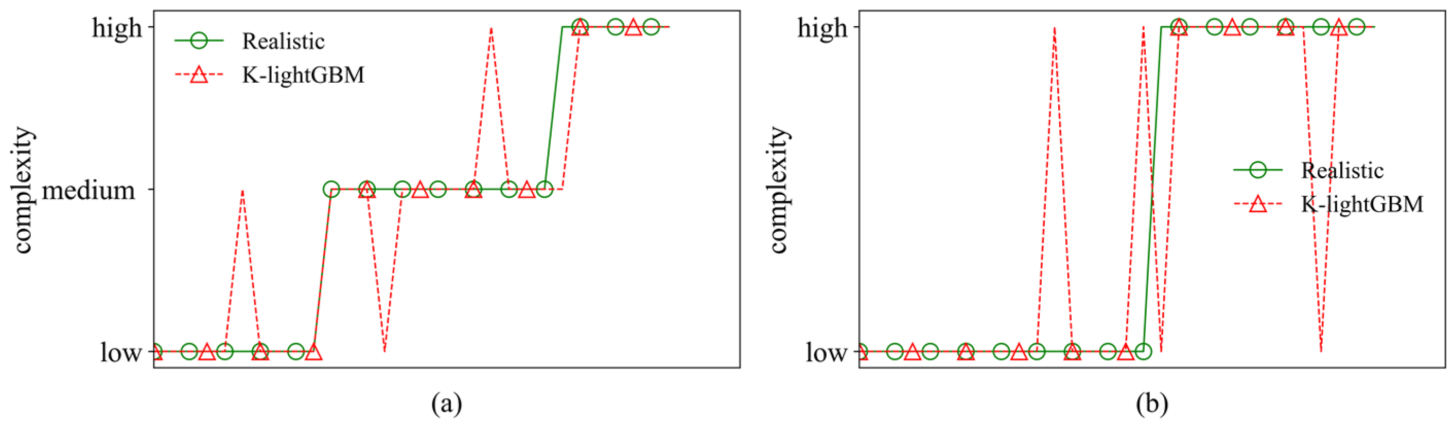
Then, the dataset of the QC handling network was divided into a 70% training set and a 30% test set. The same treatment is done for the dataset of the YC handling network. Figure 6 shows the test sets results of the QC and YC handling networks.

It can be seen that the results of these two models are the same. The accuracy of the QC handling network and the YC handling network in the test set has reached 90%. It is shown that the K-LightGBM model can accurately identify the complexity of multi-level handling.

5.3. Predicting the Handling Complexity

The obtained feature data of the handling complexity of the QC/YC handling network are numbered from n₁ to n₉₈. The data from n₁ to n₆₈ are used as ARIMA-LightGBM inputs. Then, we can get the data of the residuals from n₁ to n₆₈. We predict residuals from n₇₀ to n₉₈ data and evaluate the effectiveness of model predictions.

The residual dataset R is constructed based on the residuals from n₁ to n₆₈ as in Equation (27). The residuals from n₁₀ to n₆₉ are used as outputs, and the first nine residual data from n₁₀ to n₆₈ are used as inputs. ARIMA-LightGBM is trained on two residual prediction strategy datasets R and predicts residuals from n₇₀ to n₉₈.

$$R=\left(\begin{array}{ccc}\begin{array}{cc}{r}_1& r_2\\ r_2& r_3\end{array}& \cdots & \begin{array}{cc}{r}_9& r_{10}\\ r_{10}& r_{11}\end{array}\\ ⋮& \ddots & ⋮\\ \begin{array}{cc}{r}_{59}& r_{60}\\ r_{60}& r_{61}\end{array}& \cdots & \begin{array}{cc}{r}_{67}& r_{68}\\ r_{68}& r_{69}\end{array}\end{array}\right)$$

(26)

In order to improve the accuracy of the predicted values of the handling complexity of automated terminals, a GD-TR based hyper-heuristic algorithm is utilized to assign appropriate weights to the predicted values of the residuals from n₇₀ to n₉₈ under two residual strategies.

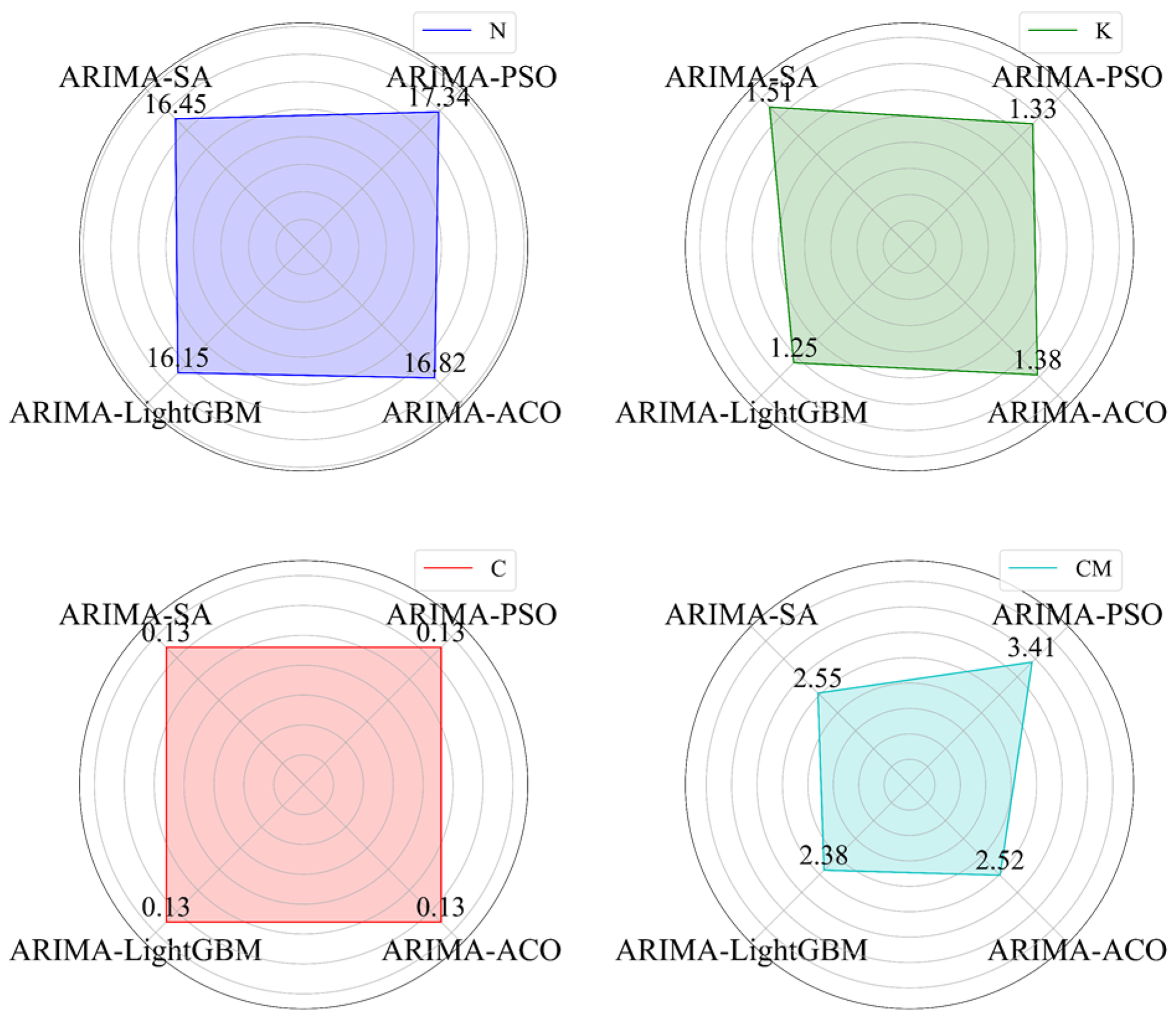
In order to be able to verify the merits of the hyper-heuristic algorithm, an experimental comparison is made by comparing the RMSE with the ARIMA-SA, ARIMA-PSO, ARIMA-ACO, and ARIMA-LightGBM for the data from n₇₀ to n₉₈. The ARIMA-SA, ARIMA-PSO, ARIMA-ACO, and ARIMA-LightGBM are the models that the SA, PSO, ACO, and hyper-heuristic algorithm assign weights to the two residual prediction strategies. The results are shown in Figure 7 and Figure 8.

It can be seen in Figure 7 and Figure 8, the RMSE of the hyper-heuristic algorithm is lower than that of SA/PSA/ACO alone.

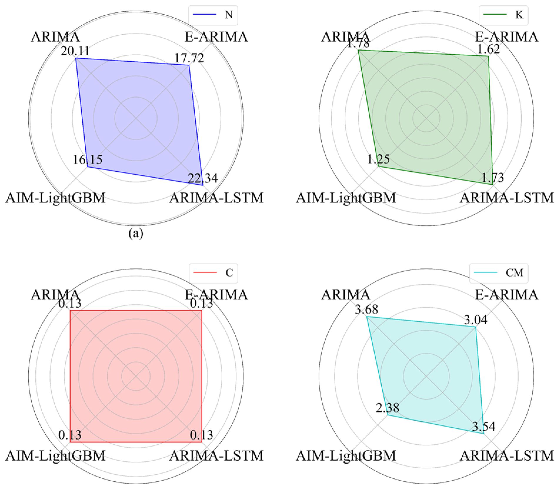
In order to be able to reflect the advantages and disadvantages of the prediction method for nonlinear data, a comprehensive evaluation is made by comparing the RMSE of the predicted values with those of ARIMA, an ARIMA fusion (ensemble of ARIMA, E-ARIMA) model [15], and an ARIMA-LSTM fusion model [16] for the data from n₇₀ to n₉₈. The results are shown in Figure 9 and Figure 10.

It can be seen in Figure 9 and Figure 10, ARIMA-LightGBM has the lowest RMSE on all features. The RMSE of the E-ARIMA model on multiple features appears to be higher than that of ARIMA-LightGBM. It can be seen that the ARIMA-based hybrid model has a great advantage on time series predictions with small data volumes and is suitable for handling complexity predictions. The ARIMA-LightGBM model, with the improvement of ARIMA, has a high prediction accuracy for handling complexity.

The data for the next 2 h are predicted based on the proposed ARIMA-LightGBM model. Taking the first nine residual data from n₉₉ to n₁₀₄ as inputs, data n₉₉ to n₁₀₄ can be obtained. We construct the residual prediction dataset R_pre according to Equation (27).

$$R_{pre}=\left(\begin{array}{ccc}\begin{array}{cc}{r}_{90}& r_{91}\end{array}& \cdots & \begin{array}{cc}{r}_{98}& r_{99}\end{array}\\ ⋮& \ddots & ⋮\\ \begin{array}{cc}{r}_{95}& r_{96}\end{array}& \cdots & \begin{array}{cc}{r}_{103}& r_{104}\end{array}\end{array}\right)$$

(27)

Because the data in

Table 1. Forecast data for the next 2 h of QC handling network.

Time	N	K	C	CM	Model
16:20	38.10	3.05	0.08	1.41	low
16:40	39.82	3.23	0.09	1.40	low
17:00	47.24	3.50	0.09	1.38	low
17:20	50.86	3.90	0.10	4.17	medium
17:40	52.85	3.53	0.12	4.18	medium
18:00	50.70	3.76	0.11	4.04	medium

and

Table 2. Forecast data for the next 2 h of YC handling network.

Time	N	K	C	CM	Model
16:20	59.33	2.25	0.07	3.56	low
16:40	73.14	2.66	0.08	3.43	high
17:00	75.80	2.91	0.13	4.37	high
17:20	73.19	3.08	0.09	3.82	high
17:40	75.81	3.06	0.12	4.28	high
18:00	72.56	3.20	0.06	3.63	high

are the final predicted values, these are not integers. From Table 1, it is found that the number of QCs and AGVs participating in operations in the QC handling network increases with time and stays around 50, and the number of QCs with more than 10 tasks increases to four. Based on the predicted values, we can assign the tasks from 17:20–18:00 in the QC processing network to 16:20–17:00 to equalize the handling complexity from 16:20–18:00.

From Table 2, it is found that the number of YCs and AGVs participating in operations in the YC handling network stays around 70, and the number of YCs with more than 10 tasks stays at four. The YC handling network had been experiencing a consistently high level of complexity since 16:40. After 16:40, the YC handling network had high handling complexity. The YC handling network presents high handling complexity because the yard is performing transloading operations while loading and unloading ships.

6. Conclusions

Monitoring and predicting the handling complexity in automated terminals can reflect whether the scheduling strategy of the automated terminals still needs to be improved. A data-driven study of multi-level operations in automated terminals can help automated terminals achieve intelligent operations and maintenance. Compared with traditional operations and maintenance, it has advantages in labor costs, data governance, etc., making automated terminal operations and maintenance no longer limited to human experience.

In this paper, we developed a study on the handling complexity of automated terminals in conjunction with complex network theory. Firstly, a automated terminal handling network was constructed according to the characteristics of automated terminal equipment operations. This paper used network topology characterization to characterize automated terminal handling complexity. An ARIMA-LightGBM model was designed to make the initial prediction of automated terminal handling complexity based on the available handling complexity data. Then, based on two residual prediction strategies, the residuals of the initial prediction of automated terminal handling complexity were predicted. We then built a hyper-heuristic algorithm architecture based on GD-TR and calculated the residual weights under two residual prediction strategies. From there, the initial handling complexity prediction results were corrected and the final handling complexity prediction was determined.

Scheduling algorithms will be added in subsequent research to perform situational awareness while scheduling operations at automated terminals. The evaluation of the situational awareness for the scheduling algorithms will be fed back to the scheduling algorithms to optimize the scheduling algorithms.