Multi-Objective Optimization for Thrust Allocation of Dynamic Positioning Ship

Abstract

Thrust allocation (TA) plays a critical role in the dynamic positioning system (DPS). The task of TA is to allocate the rotational speed and angle of each thruster to generate the generalized control forces. Most studies take TA as a single-objective optimization problem; however, TA is a multi-objective optimization problem (MOP), which needs to satisfy multiple conflicting allocation objectives simultaneously. This study proposes an improved multi-objective particle swarm optimization (IMOPSO) method to deal with the non-convex MOP of TA. The objective functions of reducing the allocation error, and minimizing the power consumption and the tear-and-wear of thrusters under physical constraints, are established and solved via MOPSO. To enhance the global seeking ability, the improved mutation strategy combined with the roulette wheel mechanism is adopted. It is shown through test data that IMOPSO converges better than multi-objective algorithms such as MOPSO and nondominated sorting genetic algorithm II (NSGA-II). Simulations are conducted for a DP ship with two propeller–rudder combinations. The simulation results with the single-objective PSO algorithm show that the proposed IMOPSO algorithm reduces thrust allocation errors in the three directions of surge, sway, and yaw by 48.48%, 39.64%, and 15.02%, respectively, and reduces power consumption by 44.53%, which demonstrates the feasibility and effectiveness of the proposed method.

1. Introduction

The dynamic positioning system (DPS) has become an essential facility for deep-sea exploration and resource development, and has been widely applied in drilling, exploration, and pipeline laying operations [1]. Dynamic positioning in the maritime industry is known as a control procedure that automatically maintains the vessel and ship position and heading direction by using its own propellers and thrusters [2]. A ship equipped with this kind of automatic control system offers a capability of holding itself stationary while retaining performance for other tasks. The DPS utilizes thrusts generated by its own thrusters to counteract environmental disturbances due to wind, waves, and currents, thereby maintaining the position and heading of the ship [3]. The control system composed of the motion controller and the thrust allocation (TA) is the core of DPS. The task of TA unit is to allocate the generalized control commands calculated by the motion controller to the individual thruster in a rational manner. The output of TA is the required thrust and azimuth angle of each thruster, providing the DP ship with the necessary control forces and moment to resist external environmental disturbances and realize the objective of DP [4]. Additionally, to ensure the operation safety of DP ship, the number of thrusters installed on a DP ship is usually greater than the required number of degrees of freedom, making the ships over-actuated and the thruster system redundant. Therefore, the TA problem can be viewed as an optimization problem that aims to determine the optimal combination of thrusters to effectively achieve the allocation objectives.

Optimization methods for TA have gained extensive attention in recent years. At the early stage, traditional gradient-based models such as linear programming (LP) [5], quadratic programming (QP) [5], and sequential quadratic programming (SQP) [6,7] algorithms have been commonly used. When dealing with TA problems where the goal is to find the most efficient and least power-consuming combination among multiple thrust and angle combinations provided by an individual thruster [8], TA can be regarded as an unconstrained least-squares optimization problem. In this situation, it can yield explicit solutions. In practice, the thrust generated by each thruster is often limited by their physical characters; thus, TA becomes a constrained optimization problem. Johansen et al. proposed an explicit solution for parametric QP to marine ships [9]. Sørdalen et al. proposed an iterative approach to solving QP problems [10]. Moreover, when azimuth thrusters are presented onboard a ship, TA problems often become non-convex and nonlinear optimization problems. Liang et al. proposed a method for optimal control of the thruster system using the quadratic sequence method [11]. De compared pseudo-inverse algorithms and QP algorithms by selecting the thrust and angle of the thrusters as design variables in the optimization problem [12]. These algorithms, when dealing with multi-objective optimization problems (MOPs) for ships, cleverly convert complex multi-objective problems into more intuitive single-objective problems (SOPs) by assigning appropriate weights to each objective. This conversion not only reduces the complexity of the problem, but also makes the optimization process easier to understand and operate. However, although these algorithms show strong local optimization ability in solving constrained nonlinear thrust allocation problems, they are weak in the global search for optimal solutions.

The rise of modern metaheuristic algorithms—such as particle swarm optimization (PSO) [13], genetic algorithm (GA) [14], artificial bee colony (ABC) algorithm [15], etc.—have effectively overcome the limitations of solution space characteristics (convex or non-convex) and initial solutions, thus exhibiting strong applicability to solve various optimization problems. Among them, PSO is an evolutionary stochastic search algorithm derived by the foraging behavior of bird flocks. Due to its simple implementation, fast convergence speed, and few parameters adjustment, it has been widely used in various areas. To balance between the local search capabilities during the evolutionary process, scholars have proposed many improved PSO algorithms to deal with the TA problem. For example, Xu et al. proposed a chaotic PSO algorithm combined with a multi-agent scheme [16], Yan proposed a hybrid optimization algorithm combining PSO with simulated annealing (SA) algorithm [17], and Ji et al. proposed a quantum-behaved particle swarm optimization algorithm (QPSO) and applied it to the thrust allocation problem [18]. Researches have verified the effectiveness of PSO on TA problem solving.

For the TA problem, the optimization model usually includes three elements: the objective function, the decision variables, and the constraints. The optimization objectives of TA are usually derived to reduce allocation error, minimize fuel consumption and minimize thruster wear-and-tear. The above studies generally combine these optimization objectives as a single objective function. However, these objectives may be conflicting such that the solution obtained is not always the optimal solution, and the optimal value may lack practical physical meanings. Actually, the TA problem is a multi-objective optimization problem in engineering application, which means that TA needs to satisfy these objectives (usually competing) simultaneously. MOPs are composed of multiple objectives. Since the multiple objectives are usually conflicting, the key to solving MOPs is to find a relatively balanced set of solutions, namely, non-dominated solutions. In order to enable PSO to solve MOPs, the multi-objective particle swarm optimization (MOPSO) algorithm was proposed by Coello et al. on the basis of PSO and the multi-objective optimization principle [19]. Although the PSO has the advantages of fast convergence speed and high search efficiency, the problems of insufficient diversity and easy falling into local optimum exist. To deal with these problems, Yang et al. proposed a dual-strategy dynamic MOPSO algorithm that can accelerate the convergence speed and increase the population diversity in dynamic environments [14]. Zhao et al. introduced angle penalty distance and an algorithm parameter self-adaptive adjustment strategy into the MOSPO algorithm, which greatly improves the search capability and optimization rate [20]. For the multi-objective TA problems, Mou et al. proposed an improved adaptive non-dominated sorting genetic algorithm III (INSGA-III) algorithm applied to ship thrust allocation, which reduced computational complexity associated with non-dominated sorting, thus reducing energy consumption [21]. Li proposed a multi-objective feasibility-enhanced particle swarm optimization algorithm (MOFEPSO) [22], which employs the self-organizing map (SOM) technique to mine the Pareto data set. In this study, a remote operated vehicle (ROV) equipped with three azimuth propellers and two fixed pitch propellers is taken as the simulation plant, and the MOP is established utilizing the thruster forces and the azimuth angles as the decision variables; thus, this approach can determine the optimal forces exerted by each thruster alone but does not directly provide the rotation speeds and rudder angles associated with each thruster.

Based on the preceding analysis, this paper presents an improved MOPSO (IMOPSO) algorithm to address the TA problem in DPS. The main contributions of this paper are as follows:

• The TA optimization problem is approached from a multi-objective perspective, where the TA objective functions are built to simultaneously minimize the thrust allocation error, power consumption, and wear-and-tear of the thruster system, taking the thruster input parameters of the propeller speed, azimuth angle, and rudder angle as decision variables. This method enables system optimization with multiple objectives in mind and helps to integrate the impact of multiple factors on system performance.
• The MOPSO algorithm is introduced to solve the TA optimization problem. The MOPSO algorithm introduces the mechanism of crowding distance and roulette method to select the globally optimal particles, and improves the inertia weights and learning factors while incorporating mutation operations to enhance the local optimization capability. The proposed IMOPSO algorithm uniquely balances the conflicting objectives of reducing allocation error, minimizing power consumption, and minimizing wear-and-tear through its particle swarm optimization mechanism, Pareto-based multi-objective strategy, elitist preservation, and constraint handling capabilities. This makes it superior to traditional multi-objective algorithms in solving multi-objective optimization problems for ships. Simulations demonstrate that the proposed algorithm exhibits a notably fast iteration speed, excellent convergence performance, and the ability to maintain population diversity. Moreover, when compared to the single-objective PSO algorithm, the proposed IMOPSO TA algorithm can reduce the thrust allocation errors, the thruster power consumption, and the changing rate of thruster inputs.
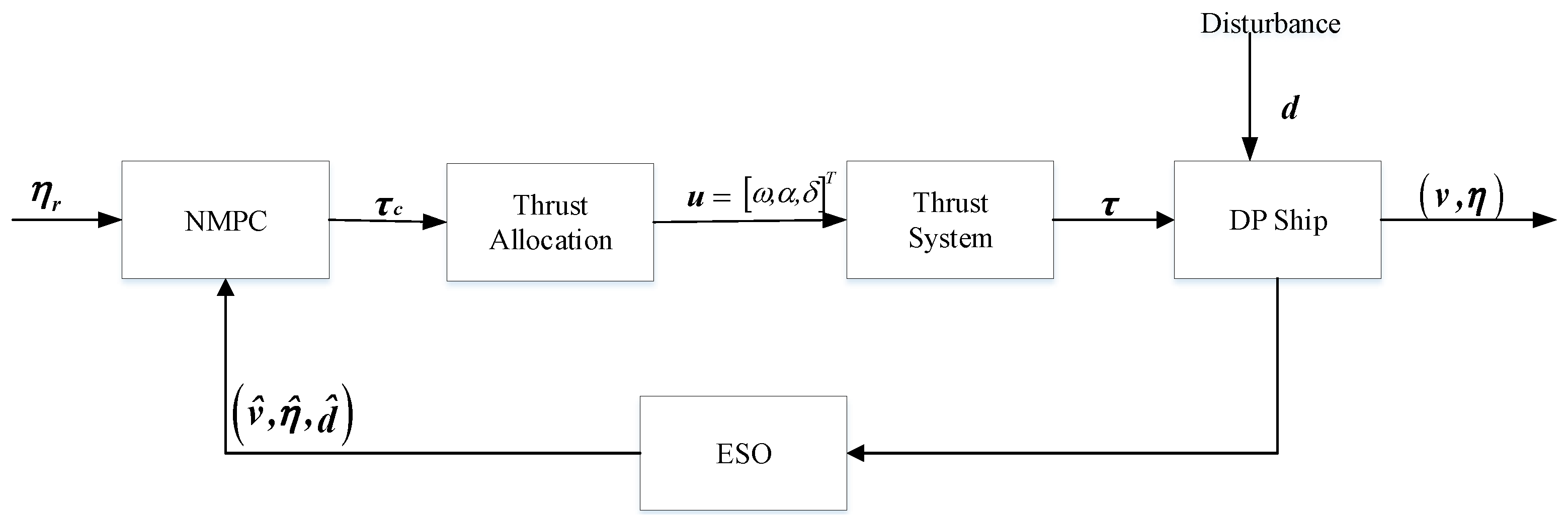
• Considering the TA under closed-loop control, a nonlinear model predictive control (NMPC) algorithm and extended state observer (ESO) are introduced. By utilizing the predictive power of NMPC and the ability of ESO to provide real-time estimation of uncertain model parameters and external disturbances, this combined approach enables accurate prediction of ship dynamics. This not only ensures TA execution accuracy but also optimizes performance by reducing allocation errors, power consumption, and equipment wear. Simulation results demonstrate the effectiveness of the proposed IMOPSO algorithm for TA in DP control systems, highlighting its potential to improve the safety, efficiency, and reliability of offshore operations.

The other paragraphs of this paper are organized as follows. In Section 2, the DP ship mathematical and thrust allocation model is analyzed. In Section 3, the improvement strategies and methods for MOPSO are proposed. Simulations are implemented to verify the feasibility of IMOPSO, which is simulated and compared with the PSO in Section 4. The conclusions are presented in Section 5.

2. Problem Formulation and Model

2.1. Preliminaries

The key differentiation between a single-objective optimization problem (SOP) and MOP lies in the number of objective functions and optimal solutions they encompass. An SOP is solved with a unique and certain optimal solution, whereas an MOP with multiple objective functions needs to be solved by simultaneously weighing up two or more conflicting objectives, in order to obtain a set of optimal solutions that do not dominate over each other [23].

An MOP with n decision variables and m objective functions can be mathematically represented by the following equation [24]:

$$\begin{array}{cc}\hfill & Min:F\left(x\right)=(f_1\left(x\right),f_2\left(x\right),\cdots ,f_m\left(x\right))\hfill \\ \hfill & s.t\hfill \\ \hfill & g_j\left(x\right)\le 0,j=1,2,\cdots k\hfill \\ \hfill & h_j\left(x\right)=0,j=1,2,\cdots l\hfill \\ \hfill & x=(x_1,x_2,\cdots x_n)\hfill \\ \hfill & x_i^{min}\le x_i\le x_i^{max},i=1,2\cdots n\hfill \end{array}$$

(1)

where $x=(x_1,x_2,\cdots x_n)\in X\subseteq R^n$ is the n dimensional decision vector, X is the feasible domain of the decision variable, $f_i\left(x\right),i=1,2\cdots m$ is the i objective function, $g_j\left(x\right)$, $j=1,2\cdots k$ is the j inequality constraint, $h_j\left(x\right),j=1,2\cdots l$ is the j equation constraint, and $x_i^{min},x_i^{max},i=1,2\cdots k$ are the maximum and minimum values of each dimensional decision variable.

Definition 1. 

Feasible solution set [25]: in the decision space, denote the set of feasible solutions by Ω, which is defined as follows:

$$\Omega =\left\{x\in R^n|g_i\le 0,i=1,2,\cdots ,k;h_j=0,j=1,2,\cdots l\right\}$$

(2)

Definition 2. 

Pareto dominance [26]: for any two solutions $x_1,x_2$ in the set of feasible solutions of the objective function $F\left(x\right)$, the dominance relation is defined as follows:

$$\begin{array}{c}\hfill x_1,x_2\in X:x_1\prec x_2\iff \left\{\forall i\in \{1,2,\cdots ,m\}:f_i\left(x_1\right)\le f_i\left(x_2\right)\right\}\\ \hfill \cup \left\{\forall j\in \{1,2,\cdots ,m\}:f_j\left(x_1\right)<f_j\left(x_2\right)\right\}\end{array}$$

(3)

where ≺ denotes domination and $x_1$ dominates $x_2$; then, $x_1$ has at least one objective function value that is better than $x_2$ and all of $x_1$ objective function values are not worse than $x_2$.

Definition 3. 

Pareto optimal [19]: for a solution $x^{*}$ in the feasible domain, $x^{*}$ is said to be a Pareto optimal solution if $x^{*}$ is not dominated by any other solution in the feasible domain, which is defined as follows:

$$\nexists x\in \Omega :x\prec x^{*}$$

(4)

Definition 4. 

Pareto optimal set [19]: the set consisting of all non-dominated solutions in the feasible domain is called the Pareto optimal set ($P_s$), which is defined as follows:

$$P_s=\left\{x^{*}|\nexists x\in \Omega ,:x\prec x^{*}\right\}$$

(5)

Definition 5. 

Pareto front [19]: the Pareto front (PF) is a surface that represents the objective function corresponding to all Pareto optimal solutions within the Pareto optimal set $P_s$, which is defined as follows:

$$PF=\left\{F\left(x^{*}\right)=(f_1\left(x^{*}\right),f_2\left(x^{*}\right),\cdots ,f_d\left(x^{*}\right))|x^{*}\in P_s\right\}$$

(6)

2.2. DP Ship Mathematical Model

For DP ships, the mathematical model for ship motion is typically nonlinear and considers only the three degrees of freedom in the horizontal plane: surge, sway, and yaw. It can be described as [27]:

$$\begin{array}{cc}\hfill \dot{\mathit{\eta }}& =\mathit{R}\left(\psi \right)\mathit{\nu },\hfill \\ \hfill \mathit{M}\dot{\mathit{\nu }}& =-\mathit{D}\left(\nu \right)\mathit{\nu }+{\mathit{\tau }}_c+\mathit{R}\left(\psi \right)\mathit{d}\hfill \end{array}$$

(7)

where $\mathit{\eta }={[x,y,\psi ]}^T$ is the vector of position and heading angle; $\nu ={[u,v,r]}^T$ is the surge, sway, and yaw velocities; ${\mathit{\tau }}_c={[F_{Xc},F_{Yc},F_{Nc}]}^T$ represents the vector of generalized forces determined by the motion controller, encompassing the combined thrust forces and moments generated by the thrust system; $\mathit{d}={[d_1,d_2,d_3]}^T$ is the vector of slow-varying disturbance forces and moments; $\mathit{M}\in {\mathbb{R}}^{3\times 3}$ is inertia matrix; $\mathit{D}\in {\mathbb{R}}^{3\times 3}$ is the damping matrix; and $\mathit{R}\left(\psi \right)$ is the rotation matrix, which are defined as

$$\begin{array}{ccc}\hfill \mathit{M}=& \left(\begin{array}{ccc}m-X_{\dot{u}}& 0& 0\\ 0& m-Y_{\dot{v}}& m{x}_g-Y_{\dot{r}}\\ 0& m{x}_g-Y_{\dot{r}}& I_z-N_{\dot{r}}\end{array}\right),\hfill & \mathit{D}=\left(\begin{array}{ccc}-X_u& 0& 0\\ 0& -Y_u& -Y_r\\ 0& -N_v& -N_r\end{array}\right)\hfill \\ \hfill \mathit{R}\left(\psi \right)=& \left(\begin{array}{ccc}cos\psi & -sin\psi & 0\\ sin\psi & cos\psi & 0\\ 0& 0& 1\end{array}\right)\hfill \end{array}$$

(8)

where m is the ship mass, $x_g$ is the center of gravity coordinate, $I_z$ is the inertia of rotation. $X_{\left(·\right)}$, $Y_{\left(·\right)}$, and $N_{\left(·\right)}$ are referred to as hydrodynamic derivatives.

The following assumptions are adopted throughout this paper.

Assumption 1. 

All the ship state variables, including positions, heading, and velocities, are measurable or can be accurately estimated.

Assumption 2. 

Since the ocean environment is slowly changing and has finite energy, the disturbances $\mathit{d}={[d_1,d_2,d_3]}^T$ acting on the ship are assumed to be time-varying yet bounded with finite changing rate. Thus, there exists an unknown positive constant ε such that $\parallel \dot{\mathit{d}}\parallel \le \epsilon$.

2.3. Mathematical Model of Thrust Allocation

In order to ensure safety and efficient motion control, DP ships are typically equipped with redundant thrusters. The thrust allocation problem requires solving for the rotational speed and rudder angle of each thruster based on the forces and moments computed by the controller, so that the thrusters produce the surge force $F_{Xc}$, the sway force $F_{Yc}$, and the yaw moment $F_{Nc}$ desired by the controller. These thrusters can be combined in various ways to generate the required generalized forces. Therefore, it is essential to solve the TA problem to determine the optimal combination of thrusters. Mathematically, the TA problem can be formulated using the following equation:

$${\mathit{\tau }}_c=B\left(\mathit{\alpha }\right)T\left(\mathit{u}\right)$$

(9)

where ${\mathit{\tau }}_c={[F_{Xc},F_{Yc},F_{Nc}]}^T$ is the desired control force generated by thrusters; the magnitude of the thrust is represented by the thrust vector $T\left(\mathit{u}\right)={[T_1,T_2,\cdots T_n]}^T$, which is a function of the thruster input $\mathit{u}={[\mathit{\omega },\mathit{\delta },\mathit{\alpha }]}^T$, where $\mathit{\omega }={[{\omega }_1,{\omega }_2\cdots {\omega }_n]}^T\in {\mathbb{R}}^n$, $\mathit{\delta }={[{\delta }_1,{\delta }_2\cdots {\delta }_n]}^T\in {\mathbb{R}}^n$, and $\mathit{\alpha }={[{\alpha }_1,{\alpha }_2\cdots {\alpha }_n]}^T\in {\mathbb{R}}^n$ are the propeller speed, rudder angle, and azimuth angle vectors, respectively. $B\left(\mathit{\alpha }\right)\in {\mathbb{R}}^{3\times n}$ is the configuration matrix of the thruster, which is defined as [22]

$$\begin{array}{c}\hfill B\left(\mathit{\alpha }\right)=\left[\begin{array}{cccc}& cos\left({\alpha }_1\right)& \cdots & cos\left({\alpha }_n\right)\\ & sin\left({\alpha }_1\right)& \cdots & sin\left({\alpha }_n\right)\\ & -l_{x1}sin\left({\alpha }_1\right)+l_{y1}cos\left({\alpha }_1\right)& \cdots & -l_{xn}sin\left({\alpha }_n\right)+l_{yn}cos\left({\alpha }_n\right)\end{array}\right]\end{array}$$

(10)

where $l_{xn},l_{yn}$ are the positions of the propellers in the hull coordinate system, respectively.

2.4. Multi-Objective Problem of Thrust Allocation

In DP ships, due to the limitation of the propellers’ own physical characteristics, the propellers may not be able to match the commanded thruster inputs immediately—i.e., propeller speed and azimuth angle—to produce the required generalized force ${\mathit{\tau }}_c$ at the current moment; so, the slack variable $\mathit{s}$ is introduced to ensure that a feasible solution of the TA problem exists. The slack variable can also be regarded as the thrust allocation error, which can be expressed as

$$\mathit{s}={\mathit{\tau }}_c-B\left(\mathit{\alpha }\right)T\left(\mathit{u}\right)$$

(11)

where $\mathit{s}={[s_X,s_Y,s_N]}^T$ is defined as the discrepancy between the generalized control force and the actual thrust generated by the thrusters.

On the basis of minimizing the thrust allocation error as much as possible, it is crucial for TA to decrease the energy consumption of the thruster system, which is often measured by the power magnitude in practical applications. For propellers and azimuth thrusters, the power consumption P is proportional to the $3rd/2$ power of thrust force, i.e., $P\propto T^{3/2}$ [28]. Further, considering that the thrust force is proportional to the square of the rotational speed, i.e., $T\propto {\omega }^2$ [29], the specific energy consumption is proportional to the $3rd$ power of the rotational speed, i.e., $P\propto {\omega }^3$. Thus, the TA objective function for minimizing the thrust allocation error and the energy consumption can be described as

$$f_1\left(\mathit{u}\right)=\sum _{i=1}^m{h}_k{\left|{\mathit{\omega }}_k\right|}^3+{\mathit{s}}^T\mathit{Q}\mathit{s}$$

(12)

where $f_1(·)$ is the first thrust allocation objective function, the first term of $f_1(·)$ represents the power consumption of thrust system and the second term represents the thrust allocation error, $h_k$ is the number of normals, ${\mathit{w}}_k$ is the propeller speed of each thruster, $k=1,2,\cdots m$ is the thruster number, and $\mathit{Q}>0$ is the definite weight matrix.

Furthermore, it is essential to minimize the wear-and-tear of thrusters. As such, the rate of change for both thruster speed and azimuth angle should not be excessively high. Hence, another thrust allocation objective function aimed at reducing the rate of change in thruster inputs and minimizing thrust allocation errors can be formulated as follows:

$$f_2\left(\mathit{u}\right)=\Delta {\mathit{u}}^T\mathit{R}\Delta \mathit{u}+{\mathit{s}}^T\mathit{Q}\mathit{s}$$

(13)

where $f_2(·)$ is the second thrust allocation objective function, $\Delta \mathit{u}$ is the thruster input increment between the current and the previous time step, and $\mathit{R}>0$ is the positive definite weights matrix.

The inequality constraints for the TA problem are mainly related to the mechanical characteristics of the thrusters, including the thruster input magnitude and the increment limitations of the propeller speed, the azimuth angle, and the rudder angle, which can be represented as

$$\left\{\begin{array}{c}{{\mathit{\alpha }}_i}^{min}\le {\mathit{\alpha }}_i\le {{\mathit{\alpha }}_i}^{max}\hfill \\ \Delta {{\mathit{\alpha }}_i}^{min}\le {\mathit{\alpha }}_i-{\mathit{\alpha }}_{0i}\le \Delta {{\mathit{\alpha }}_i}^{max}\hfill \\ {\mathit{\delta }}_i^{min}\le {\mathit{\delta }}_i\le {\mathit{\delta }}_i^{max}\hfill \\ \Delta {\mathit{\delta }}_i^{min}\le {\mathit{\delta }}_i-{\mathit{\delta }}_{0i}\le \Delta {\mathit{\delta }}_i^{max}\hfill \\ {\mathit{\omega }}_i^{min}\le {\mathit{\omega }}_i\le {\mathit{\omega }}_i^{max}\hfill \\ \Delta {\mathit{\omega }}_i^{min}\le {\mathit{\omega }}_i-{\mathit{\omega }}_{0i}\le \Delta {\mathit{\omega }}_i^{max}\hfill \end{array}\right.$$

(14)

where ${\mathit{\alpha }}_{\mathit{i}}^{min}$, ${\mathit{\delta }}_i^{min}$, and ${\mathit{\omega }}_i^{min}$ are the minimum values of the azimuth angle, the rudder angle, and the propeller speed, respectively; ${\mathit{\alpha }}_{\mathit{i}}^{max}$, ${\mathit{\delta }}_{\mathit{i}}^{max}$, and ${\mathit{\omega }}_{\mathit{i}}^{max}$ are the maximum values of the azimuth angle, the rudder angle, and the propeller speed, respectively; $\Delta {\mathit{\alpha }}_{\mathit{i}}^{min}$, $\Delta {\mathit{\delta }}_i^{min}$, and $\Delta {\mathit{\omega }}_i^{min}$ are the minimum values of rate of the change of the azimuth angle, rate of change of the rudder angle, and rate of change of the propeller speed, respectively; and $\Delta {\mathit{\alpha }}_{\mathit{i}}^{max}$, $\Delta {\mathit{\delta }}_i^{max}$, and $\Delta {\mathit{\omega }}_i^{max}$ are the maximum values of rate of change of the azimuth angle, rate of change of the rudder angle, and rate of change of the propeller speed, respectively. Based on the above analysis, the MOP objective function for DP thrust allocation can be established according to Equations (11)–(14) as follows:

$$\begin{array}{cc}\hfill Min:& F\left(\mathit{u}\right)=(f_1\left(\mathit{u}\right),f_2\left(\mathit{u}\right))\hfill \\ \hfill s.t.& \left\{\begin{array}{c}\mathit{s}={\mathit{\tau }}_c-B\left(\mathit{\alpha }\right)T\left(\mathit{u}\right)\hfill \\ {{\mathit{\alpha }}_i}^{min}\le {\mathit{\alpha }}_i\le {{\mathit{\alpha }}_i}^{max}\hfill \\ \Delta {{\mathit{\alpha }}_i}^{min}\le {\mathit{\alpha }}_i-{\mathit{\alpha }}_{0i}\le \Delta {{\mathit{\alpha }}_i}^{max}\hfill \\ {\mathit{\delta }}_i^{min}\le {\mathit{\delta }}_i\le {\mathit{\delta }}_i^{max}\hfill \\ \Delta {\mathit{\delta }}_i^{min}\le {\mathit{\delta }}_i-{\mathit{\delta }}_{0i}\le \Delta {\mathit{\delta }}_i^{max}\hfill \\ {\mathit{\omega }}_i^{min}\le {\mathit{\omega }}_i\le {\mathit{\omega }}_i^{max}\hfill \\ \Delta {\mathit{\omega }}_i^{min}\le {\mathit{\omega }}_i-{\mathit{\omega }}_{0i}\le \Delta {\mathit{\omega }}_i^{max}\hfill \end{array}\right.\hfill \end{array}$$

(15)

Assumption 3. 

Under the given constraints, there exists at least one solution that satisfies all the objective functions and achieves optimal performance.

Remark 1. 

In traditional DP thrust allocation problems, the objectives of reducing the thrust allocation error, the energy consumption, and the wear-and-tear of thruster system are generally combined as a single objective function using the weighted-sum, i.e., $F={\omega }_1{f}_1+{\omega }_2{f}_2$. However, some of the objective functions may be conflicting and the optimal value may lack practical physical meanings. In actual engineering practice, the DP thruster system needs to satisfy the two objectives (usually competing) simultaneously. This means that the thrust allocation problem is an MOP indeed. When dealing with the MOP, the physical meanings of the aspects considered are clear, and the relationship between objectives can be investigated easily, especially for conflicting objectives.

3. The Proposed Method

3.1. Improved MOPSO (IMOPSO) Algorithm

Based on the MOP principle and the PSO algorithm proposed by Eberhart et al. [30], the MOPSO algorithm was proposed by Coello et al. [19]. The MOPSO algorithm is an evolutionary algorithm based on group intelligence. It has strong generality, which can make full use of the individual’s local optimal information and the group’s overall optimal information to deal with the MOPs in the field of engineering. In this section, the MOPSO algorithm will be specially derived to solve the thrust allocation multi-objective of DP system defined in Equation (15).

In the DP ship TA optimization problem, the characteristics of the particles are represented by three metrics: particle velocity, particle position, and fitness. The MOPSO algorithm uses the concept of Pareto domination to determine the flight direction of the particles, and the non-dominated individuals are obtained through the comparison of domination relationships between particles and stored in the global elite pool $nRep$. The global optimal solution $gbest$ is selected from the global elite pool, and the individual optimal solution $pbest$ is selected based on the comparison of dominance relationships between the old and new generations of individuals in the population. The velocity and position of the particle swarm are updated by continuous iteration, which eventually covers the entire search space and yields a non-inferior solution set close to the true PF.

3.1.1. Creation of External Archives Repository

The external archive set is the set that holds all the non-dominated solutions found by the algorithm. After setting the external archive set, the algorithm only uses the non-dominated solutions selected in each iteration to compare with the solutions in the external set according to the domination relationship; in this way, the algorithm runs faster and the global optimal solution is selected in the external solution set each time.

According to the sorting method in Deb et al. [31], the population is sorted by non-domination and the set of non-dominated solutions is constructed. In the first iteration, the set of non-dominated solutions found is directly put into the set of external archives; in the later iterations, the non-dominated solutions generated this time are compared with the original set of external archives in terms of Pareto domination relationship, the dominated solutions are removed, and the dominated solutions are added in to obtain the new set of external archives.

A maximum stock parameter is set for the external archive set, and along with the iteration, when the number of particles in the external archive set is equal to the maximum stock, in order to continue to store the better solutions, a descending order is implemented through the congestion distance ordering principle in Deb et al. [31], and the solutions with smaller congestion distances are removed from the overrun. Crowding distance is a kind of metric that uses neighboring individuals to judge whether the distance between individuals and neighboring individuals is close, i.e., whether the distribution is even (diversity); when the crowding distance is larger, the solution set is looser and the diversity of solutions is better. The formula for calculating the crowding distance is as follows:

$$C_k=\frac{1}{n}\left(\sum _{i=1}^n|f_i\left(x_{k-1}\right)-f_i\left(x_k\right)|+\sum _{i=1}^n|f_i\left(x_k\right)-f_i\left(x_{k+1}\right)|\right)$$

(16)

where $x_{k-1}$ and $x_{k+1}$ are the two individuals adjacent to the same x, respectively; $f(·)$ is the fitness function; and n is the number of objective functions.

3.1.2. Determination of Individual and Global Optimal Solutions

During each iteration, the particle is judged on the basis of the two poles currently obtained, i.e., the individual optimal solution and the global optimal solution, to determine the optimal destination of the particle. When the algorithm starts running, the individual optimum is the initial position of the particle; thereafter, as the iterative process continues, the individual optimum solution is generated based on the non-dominated solution obtained from the comparison of Pareto dominance relations. The global optimal solution is selected from the set of non-dominated solutions; the global optimal particle is selected from the $nRep$ according to the roulette method; and if there are multiple identical optimal particles, one of them is randomly selected as the global optimal particle.

3.1.3. Improvements during Particle Updates

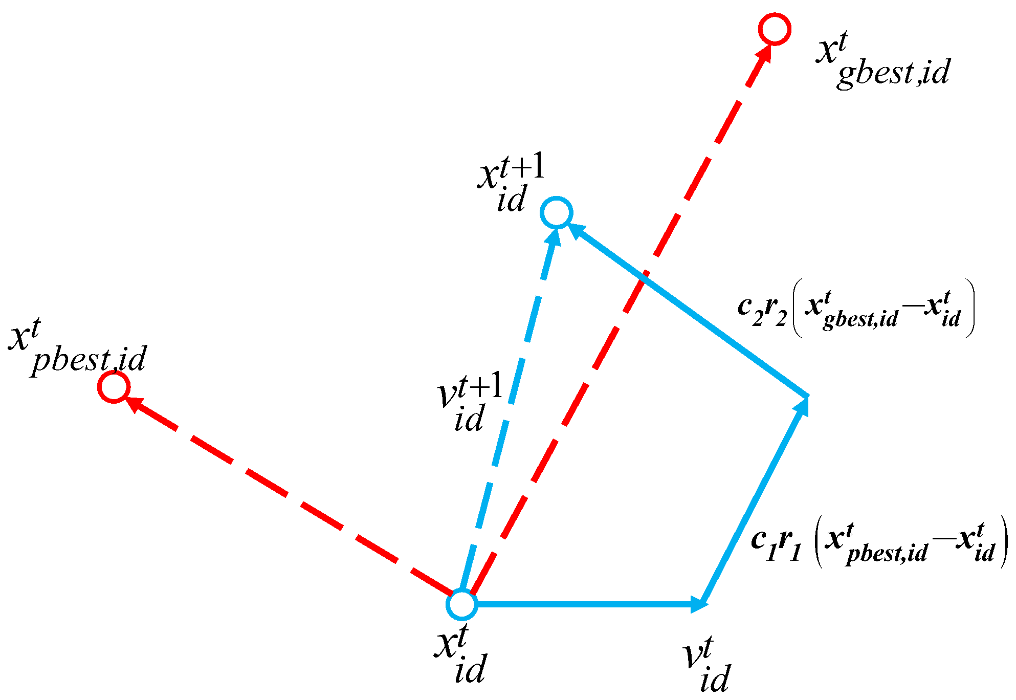
• Asynchronously changing learning rate: in the PSO algorithm, updating of particle velocity and position is defined as follows:

  $$\begin{array}{c}{v}_{id}^{t+1}=\kappa ·v_{id}^t+c_1{r}_1·(x_{pbest,id}^t-x_{id}^t)+c_2{r}_2·(x_{gbest}^t-x_{id}^t)\hfill \\ x_{id}^{t+1}=x_{id}^t+v_{id}^{t+1}\hfill \end{array}$$

  (17)
  The learning factor enables the particle to master the ability of self-learning and learning from other better particles in the optimization process, and gradually approach the optimal solution. Asynchronous change means that the two have inconsistent changes. By making the learning factors $c_1$ and $c_2$ change asynchronously, the change is as in Equation (18). This means that at the beginning of the optimization the particles are good at self-learning and relatively poor at social ability, and at the end of the optimization they are just the opposite; this practice can help the algorithm converge to the global optimal solution to prevent falling into the local optimum.
  The improved learning factor is defined as follows:

  $$\begin{array}{c}\hfill \left\{\begin{array}{c}{c}_1=(c_{1s}-c_{1e})\times \frac{m-t}{m}+c_{1e}\hfill \\ c_2=(c_{2s}-c_{2e})\times \frac{m-t}{m}+c_{2e}\hfill \end{array}\right.\end{array}$$

  (18)

  where $v_{id}^t,x_{id}^t,x_{pbest,id}^t$, and $x_{gbest,id}^t$ denote the velocity, the position, the individual best position, and the population best position of the i particles at t iterations in the d dimension, respectively. The $v_{id}^{t+1}$ and $x_{id}^{t+1}$ denote the velocity and position of the i-particle in the d-dimension at the $t+1$ iteration, respectively. $\kappa$ is the inertia weight, $r_1$ and $r_2$ are random numbers uniformly distributed between [0, 1], and $c_1$ and $c_2$ are the individual learning factor and group learning factor.
  Figure 1 shows the path diagram of the particle update, in which the velocity update of the particle mainly consists of its own velocity $v_{id}^t$, the self-knowledge part $c_1{r}_1·(x_{pbest,id}^t-x_{id}^t)$, and the social experience part $c_2{r}_2·(x_{gbest}^t-x_{id}^t)$; the position update mainly consists of the particle’s current position $x_{id}^t$ and the updated velocity $v_{id}^{t+1}$.
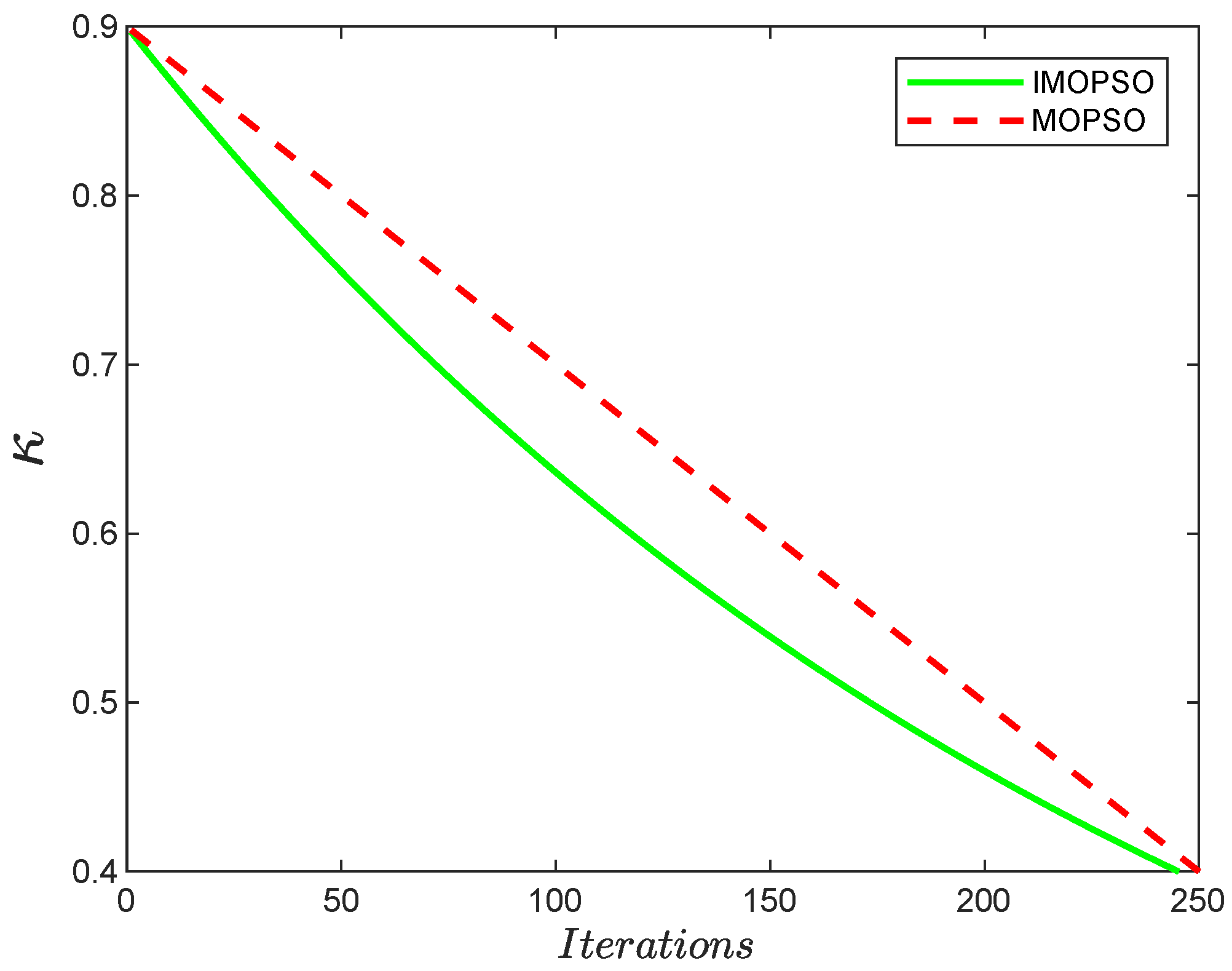
• Adjusting inertia weight: In PSO algorithm, the inertia weight $\kappa$ usually changes dynamically with the current number of iterations t. The MOPSO algorithm usually employs a linear descent strategy to enhance the algorithm’s ability to find the optimum, and the weight change equation is defined as follows:

  $$\kappa ={\kappa }_{max}-\frac{{\kappa }_{max}-{\kappa }_{min}}{m}\times t$$

  (19)

  where ${\kappa }_{max}$, ${\kappa }_{min}$ are the maximum and minimum values of $\kappa$, respectively.
  However, the search accuracy of the linear descent strategy is not high. In the optimization process, it is better to focus on the global search at the beginning and then focus on the local search at a later stage, which not only improves the convergence speed of the algorithm but also improves the search accuracy of the algorithm. Therefore, this paper proposes an inertia weight exponentially decreasing strategy, and the improved weight change formula is defined as

  $$\kappa =0.8\times e^{-\frac{t}{m}}+0.1$$

  (20)

  The trend of $\kappa$ with the number of iterations obtained from Equations (19) and (20) are shown in Figure 2.
• Mutation operation: The MOPSO algorithm can produce optimization results quickly due to its fast convergence rate. However, it may also cause particles fall into local optimal solutions; to overcome this drawback, the algorithm performs a mutation operation on the particles during the iteration process. At the beginning of the iteration, a large-scale search is required due to the large gap between the solution and the optimal solution sets in order to expand the search, increasing the probability that particle mutation is used to narrow the gap between the solution and the optimal solution sets. In the later stages of the iteration, the mutation probability of the particles is gradually reduced in order for the algorithm to converge quickly. Therefore, the mutation probability of the particle is gradually decreasing as the number of iterations increases. The mutation probability of a particle is defined as

  $$p_m={\left(1-\frac{t-1}{m-1}\right)}^{\frac{1}{\mu }}$$

  (21)

  where $p_m$ is the mutation probability of the t-th iteration, m is the maximum number of iterations of the MOPSO algorithm, and $\mu$ is the conditioning factor.

3.2. IMOPSO Algorithm Procedure

In this study, we utilize the IMOPSO algorithm to optimize the TA problem. The effectiveness of the thrust allocation scheme is assessed by taking into account two critical factors: thruster energy consumption and wear-and-tear. By integrating these criteria into the optimization process, we aim to find a thrust allocation solution that minimizes energy consumption while also minimizing wear-and-tear on the thrusters. This method not only facilitates energy conservation but also ensures the sustainable operation of the thrusters, thereby promoting their efficiency and viability. The pseudocode of the algorithm is presented in Algorithm 1.

Algorithm 1	IMOPSO algorithm optimization process
Input	Population size N.
	Number of external archives $nRep$.
	Maximum number of iterations m.
	Learning factors $c_{1s}$, $c_{1e}$, $c_{2s}$, $c_{2e}$.
	Conditioning factor $\mu$.
Output	The optimal solution of thruster input $\mathit{u}={\left[\omega \delta \alpha \right]}^T$.
1.	Initialize
2.	Generate the velocity and position of each particle according to
	the given constraints
3.	Assess the fitness value of every particle
4.	Fill the $pbest$ of each particle with its current position
5.	FOR $t=1$ : m
	FOR $i=1$ : N
	Select $gbest$
	Introduce a weighting matrix $\kappa$
	Update particle velocity $v_{id}$
	Update particle position $x_{id}$
	Perform boundary judgment
	IF $rand<p_m$
	Perform mutation operations
	END IF
	Update $pbest$
	END FOR
	Add updated particles to $nRep$
	Perform dominance analysis
	Retain non-dominated members
	Update grids and grid indexes
	Check repository fullness
	IF $num\left(Rep\right)>nRep$
	Extra= ($numel\left(Rep\right)-nRep$)
	Delete Extra
	END IF
6.	END FOR

3.3. Performance Evaluation of IMOPSO

In order to verify the feasibility and effectiveness of the proposed IMOPSO algorithm, four benchmark bi-objective functions from ZDT1 to ZDT4 are selected for testing herein. Meanwhile, in order to analyze the superiority of the IMOPSO algorithm, the simulation results are compared with results of the traditional MOPSO algorithm and nondominated sorting genetic algorithm II (NSGA-II). Each algorithm was executed 30 times for all test problems, with a population size of 100 and a maximum iteration count of 200.

In order to evaluate the convergence and diversity of the algorithm, the inverse generation distance (IGD) [24] and hypervolume (HV) [32] are chosen as assessment indices.

The IGD measures the average of the lowermost distances between the true PF individuals to the set of approximate solutions obtained by the algorithm, and the set of solutions that are uniformly sampled on a set of real PFs is obtained in advance when calculating the IGD. Let $P^{*}$ be a set of solutions uniformly sampled on the real PF and S be the set of approximate solutions to the PF obtained by the multiobjective particle swarm algorithm; then, the IGD is defined as follows:

$$IGD(S,P^{*})=\frac{{\sum }_{x\in P^{*}}dist(x,S)}{|P^{*}|}$$

(22)

where $dist(x,S)$ denotes the Euclidean distance between an individual $x\in P^{*}$ to the nearest individual on S, and $|P^{*}|$ is the cardinality of the set $P^{*}$. A smaller value of IGD denotes that S has better convergence and diversity, and can approximate the PFs as a whole.

HV is defined as a set of pre-set reference points $r^{*}=(r_1^{*},r_2^{*},\cdots ,r_m^{*})$ distributed in the target space with a set of PF approximate solutions S obtained by the algorithm, satisfying that $r^{*}$ is dominated by all the solutions in S. HV measures the size of the volume of the target space bounded by $r^{*}$ and dominated by S. HV is defined as follows:

$$HV\left(S\right)=VOL(\bigcup _{x\in S}[f_1\left(x\right),r_1^m]\times \cdots [f_m\left(x\right),r_m^{*}])$$

(23)

where $VOL(·)$ denotes the Lebesgue measure. The larger the value of HV, the better the convergence and diversity of the algorithm.

Figure 3 compares the Pareto front values calculated by IMOPSO with the true Pareto front value of ZDT1 to ZDT4 benchmark functions. It can be seen that the solutions of IMOPSO are very close to the true solution.

Table 1. The HV and IGD values of IMOPSO, MOPSO, and NSGA-II algorithms for benchmark functions.

Benchmark Function	Algorithm	HV		IGD
		Mean	Std	Mean	Std
ZDT1	IMOPSO	7.1525 $\times {10}^{-1}$	9.8272 $\times {10}^{-4}$	8.7059 $\times {10}^{-3}$	9.9005 $\times {10}^{-4}$
	MOPSO	7.0482 $\times {10}^{-1}$	2.3940 $\times {10}^{-2}$	1.8510 $\times {10}^{-2}$	2.3014 $\times {10}^{-2}$
	NSGA-II	4.5559 $\times {10}^{-1}$	7.0696 $\times {10}^{-2}$	2.5117 $\times {10}^{-1}$	8.3138 $\times {10}^{-2}$
ZDT2	IMOPSO	4.4018 $\times {10}^{-1}$	8.7641 $\times {10}^{-4}$	9.0600 $\times {10}^{-3}$	1.0592 $\times {10}^{-3}$
	MOPSO	4.3842 $\times {10}^{-1}$	2.0171 $\times {10}^{-3}$	1.0955 $\times {10}^{-2}$	1.7088 $\times {10}^{-3}$
	NSGA-II	2.5952 $\times {10}^{-1}$	6.9814 $\times {10}^{-2}$	1.8818 $\times {10}^{-1}$	1.3126 $\times {10}^{-1}$
ZDT3	IMOPSO	5.9816 $\times {10}^{-1}$	8.3284 $\times {10}^{-4}$	9.6166 $\times {10}^{-3}$	1.3557 $\times {10}^{-3}$
	MOPSO	5.8501 $\times {10}^{-1}$	3.2777 $\times {10}^{-2}$	1.4963 $\times {10}^{-2}$	9.5468 $\times {10}^{-3}$
	NSGA-II	5.0154 $\times {10}^{-1}$	5.4232 $\times {10}^{-2}$	2.9425 $\times {10}^{-1}$	6.1269 $\times {10}^{-2}$
ZDT4	IMOPSO	7.1356 $\times {10}^{-1}$	7.6873 $\times {10}^{-4}$	8.8606 $\times {10}^{-3}$	7.7719 $\times {10}^{-4}$
	MOPSO	7.0876 $\times {10}^{-1}$	2.8030 $\times {10}^{-2}$	8.8071 $\times {10}^{-3}$	1.2782 $\times {10}^{-4}$
	NSGA-II	3.7631 $\times {10}^{-1}$	1.6513 $\times {10}^{-1}$	3.2794 $\times {10}^{-1}$	1.8992 $\times {10}^{-1}$

presents the HV and IGD values of IMOPSO, MOPSO, and NSGA-II algorithms for benchmark functions. According to the data in the table, the IMOPSO algorithm performs well in terms of HV, with a larger mean value and smaller standard deviation compared to MOPSO and NSGA-II. This shows that the IMOPSO algorithm not only generates higher quality solution sets, but also maintains the diversity of solutions. In terms of IGD, the IMOPSO algorithm also has a smaller mean and standard deviation, further confirming the convergence and diversity performance of the IMOPSO algorithm.

4. Numerical Simulations and Result Discussions

4.1. Simulation Parameter Settings

To validate the efficacy of the proposed IMOPSO algorithm for DP ship thrust allocation plant, this paper conducts comparative experiments with the PSO algorithm. The ship chosen for simulation is the Cybership II (CSII), which is a 1:70 scale replica of a supply ship [27]. The prior identified dynamic parameters for CSII are defined in

Table 2. CSII ship parameters [27].

Parameter	Value	Unit	Parameter	Value	Unit
m	23.8	kg	$x_g$	0.046	m
$X_{\dot{u}}$	−2.0	kg	$Y_{\dot{\nu }}$	−10.0	kg
$Y_{\dot{r}}$	−0.0	kg·m	$N_{\dot{r}}$	−1.0	kg·m2
$I_z$	1.76	kg·m2	$X_u$	−2	kg/s
$Y_v$	−7	kg/s	$Y_r$	−0.1	kg·m/s
$N_v$	−0.1	kg·m/s	$N_r$	−0.5	kg·m/s

. The CSII ship is used as the experimental object, as shown in Figure 4. The CSII Ship is equipped with a set of rudder–propeller thrusters (No.1,2) on the port and starboard sides of the stern, and a set of lateral channel thrusters (No.3) on the bow. The azimuth angles of the aft port and starboard main propeller are fixed as ${\alpha }_{1,2}=0^{\circ }$, and the amount of side thrust is changed by changing the rudder angle. The azimuth angle of the bow channel propeller is fixed as ${\alpha }_3={90}^{\circ }$; the thrust produced by the three sets of propellers and its range are shown in

Table 3. Thruster position and related physical restrictions.

Thruster Number	${\mathit{L}}_{\mathit{x}}$	${\mathit{L}}_{\mathit{y}}$	Range of Propeller Speed (rad/s) and Rudder Angle (deg)	Change Rate of Propeller Speed (rad/s) and Rudder Angle (deg)
$\#1\mathrm{main}\mathrm{propeller}$	$-0.54$	$-0.075$	$[40,-40]$	$[8,-8]$
$\#1\mathrm{rudder}$	$-0.595$	$-0.075$	$[35,-35]$	$[3,-3]$
$\#2\mathrm{main}\mathrm{propeller}$	$-0.54$	$0.075$	$[40,-40]$	$[8,-8]$
$\#2\mathrm{rudder}$	$-0.595$	$-0.075$	$[35,-35]$	$[3,-3]$
$\#3\mathrm{channel}\mathrm{thrusters}$	$0.456$	0	$[200,-200]$	$[20,-20]$

.

The thrusts generated by the propellers consist of two parts: The first part is the thrusts generated by the stern main propeller and the channel thruster, which can be calculated as [33]

$$\begin{array}{ccc}\hfill {\mathcal{T}}_i=& \left\{\begin{array}{ccc}{k}_{iTp}{\omega }_i^2\hfill & \hfill & {\omega }_i\ge 0\hfill \\ k_{iTP}\left|{\omega }_i\right|{\omega }_i\hfill & \hfill & {\omega }_i\le 0\hfill \end{array}\right.\hfill & \hfill i\in [1\cdots 3]\end{array}$$

(24)

The second part is the lift and drag force generated by the rudder. The rudder lift force can be calculated as

$$\begin{array}{ccc}\hfill {\mathcal{L}}_i=& \left\{\begin{array}{ccc}{T}_i(1+k_{iLn}{\omega }_i)(k_{iLn{\delta }_1}+k_{iL{\delta }_2}|{\delta }_i\left|\right)){\delta }_i\hfill & \hfill & {\omega }_i\ge 0\hfill \\ 0\hfill & \hfill & {\omega }_i\le 0\hfill \end{array}\right.\hfill & \hfill i\in [1,2]\end{array}$$

(25)

The rudder drag force can be calculated as

$$\begin{array}{ccc}\hfill {\mathcal{D}}_i=& \left\{\begin{array}{ccc}{T}_i(1+k_{iDn}{\omega }_i)(k_{iL{\delta }_2}|{\delta }_i\left|\right){\delta }_i\hfill & \hfill & {\omega }_i\ge 0\hfill \\ 0\hfill & \hfill & {\omega }_i\le 0\hfill \end{array}\right.\hfill & \hfill i\in [1,2]\end{array}$$

(26)

The longitudinal and lateral thrusts generated by the rudder–propeller combination thruster system can be expressed as

$$\begin{array}{c}\hfill T_i=\left[\begin{array}{cc}{\mathcal{T}}_i-{\mathcal{D}}_i& i\in [1,2]\\ {\mathcal{T}}_i& i=3& \\ {\mathcal{L}}_i& i\in [1,2]\end{array}\right]\end{array}$$

(27)

where $k_{iTp}, k_{iTn}, k_{iLn}, k_{iLn\delta n}, k_{iD\delta n}$ are the parameters of the propeller and rudder. The values of the parameters are shown in

Table 4. Parameter values of the thruster system.

Parameter	Value	Unit
$k_{1Tp}/k_{2Tp}$	$0.00374$	N·${\mathrm{s}}^2$
$k_{3Tp}$	$0.000184$	N·$s^2$
$k_{1Tn}/k_{2Tn}$	$0.00505$	N·${\mathrm{s}}^2$
$k_{3Tn}$	$0.000188$	N·${\mathrm{s}}^2$
$k_{1Ln}/k_{2Ln}$	$0.021$	s
$k_{1L{\delta }_1}/k_{2L{\delta }_1}$	$0.927$	${\mathrm{rad}}^{-1}$
$k_{1L{\delta }_2}/k_{2L{\delta }_2}$	$-0.557$	${\mathrm{rad}}^{-2}$
$k_{1Dn}/k_{2Dn}$	$0.00964$	s
$k_{1D{\delta }_1}/k_{D{\delta }_1}$	$0.079$	${\mathrm{rad}}^{-1}$
$k_{1D{\delta }_2}/k_{2D{\delta }_2}$	$0.615$	${\mathrm{rad}}^{-2}$

.

Noting that there exist saturation constraints for the rudders, the range of thrust for the propeller–rudder combination thruster is non-convex (see Figure 4), which leads the TA optimization problem to be non-convex. The parameters of the IMOPSO algorithm are set as follows: population size $N=100$, initial value of learning factor $c_{1s}=2.5$, $c_{2s}=0.5$; final value of learning factor $c_{1e}=0.5$, $c_{2e}=2.5$; maximum number of iterations $m=200$; conditioning factor $\mu =0.1$. The relevant parameters in the TA objective function are set as follows: the power consumption constants $\mathit{h}={[9\times {10}^{-4},9\times {10}^{-4},4\times {10}^{-5}]}^T$, the slack variable weight matrix $\mathit{Q}=diag{[{10}^3,{10}^3,{10}^4]}^T$, and the thruster input increment weight matrix $\mathit{R}=diag{[0.01,0.01,0.01,0.01,0.01]}^T$.

In order to verify the performance of the algorithms, this paper compares the thrust allocation effect of the IMOPSO algorithm with that of the single-objective PSO algorithm. In the SOP thrust allocation, the two objective functions defined in Equations (12) and (13) are integrated as a single objective functions and solved using PSO. The PSO algorithm is implemented with the same parameters as the IMOPSO algorithm. All the simulations are implemented on a personal computer through the MATLAB R2022a platform. The computer is configured with an i5-12400F 2.5 GHz CPU, 16 GB of operating memory, and a 64-bit operating system.

4.2. Simulation Results and Discussions

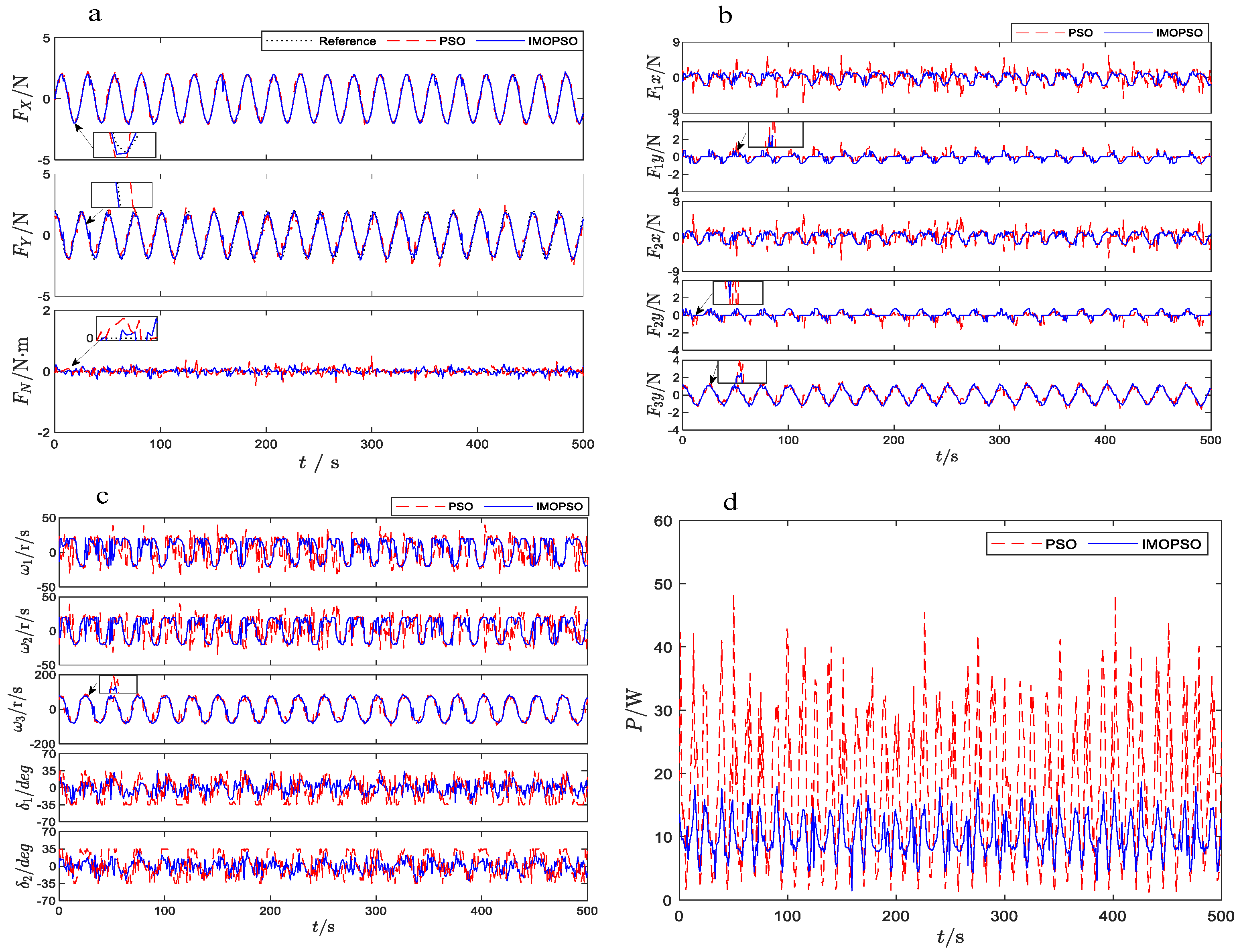
4.2.1. Thrust Allocation Performance Evaluation

Firstly, the demanded generalized force ${\mathit{\tau }}_d={[F_{Xd},F_{Yd},F_{Nd}]}^T$ are preset to verify the feasibility and effectiveness of the IMOPSO algorithm. The results are compared with those of the single-objective PSO algorithm. The preset control force and moment are defined as follows:

$$\begin{array}{c}\hfill \left\{\begin{array}{c}{F}_{Xd}=2sin\left(0.25t\right)\hfill \\ F_{Yd}=2cos\left(0.25t\right)\hfill \\ F_{Nd}=0\hfill \end{array}\right.\end{array}$$

(28)

Figure 5a shows the comparison results of the total generalized forces of thruster system determined by IMOPSO and PSO algorithms. In Figure 5a, the black dotted line represents the reference demanded generalized forces, and the solid blue and dashed red line, respectively, represent the generalized forces generated via IMOPSO and PSO thrust allocation. It can be seen that IMOPSO can track the preset forces and moments more smoothly and accurately compared with the PSO algorithm. Figure 5b shows the results of the comparison of the generalized forces for each thruster determined by the IMOPSO and PSO algorithms. In Figure 5b, the blue solid line and the red dashed line indicate the thrust provided by each thruster allocated via the IMOPSO and PSO algorithms, respectively. It can be seen that the IMOPSO algorithm performs more smoothly than the PSO algorithm when allocating thrust for each thruster. Figure 5c shows the comparison results of propeller speed and rudder angle assigned to each thruster by the IMOPSO and PSO algorithms. In Figure 5c, the blue solid line and the red dashed line indicate the propeller speed and rudder angle allocated by the IMOPSO and PSO algorithms, respectively. It can be seen that the IMOPSO algorithm has less fluctuation changes than the PSO algorithm in the feasible domain of thrusters, and the results satisfy the constraints in Table 3, which verifies the stability of the IMOPSO algorithm. Figure 5d shows the comparison results of the total thruster power consumption of the IMOPSO and PSO algorithms. In Figure 5d, the blue solid line and the red dashed line indicate the total power consumption of the IMOPSO and the PSO algorithms, respectively.

Table 5. Total power consumption of the algorithms.

Algorithms	Total Algorithm Power Consumption (kW)
PSO	$9.009$
IMOPSO	$4.997$

shows that the power consumption of IMOPSO algorithm is 4.997 kW while the power consumption of PSO algorithm is 9.009 kW; the power consumption of IMOPSO algorithm is less than the power consumption of PSO algorithm. This shows that the IMOPSO algorithm is more energy efficient and verifies the superiority of the algorithm.

To further compare the control accuracy of IMOPSO and PSO algorithms, the root mean squared error (RMSE) is defined to measure the difference between the commanded thrust and the allocated thrust. The expression of RMSE is defined as follows:

$$RMSE=\sqrt{\frac{1}{N_k}\sum _{k=1}^{N_k}({\mathit{\tau }}_c-{\mathit{\tau }}_d)}$$

(29)

where $N_k$ is the sampling time.

Table 6. Comparison of RMSE between IMOPSO and PSO algorithms.

RMSE	PSO	IMOPSO	Improvement Percentage
$F_X$	$0.297072242$	$0.153065886$	$48.48\%$
$F_Y$	$0.382903299$	$0.231104218$	$39.64\%$
$F_N$	$0.112351476$	$0.095472687$	$15.02\%$

shows the comparison of RMSE between IMOSPO and PSO algorithms. It can be observed that in comparison to the PSO algorithm, the IMOPSO algorithm results in a reduction of $48.48\%$, $39.64\%$, and $15.02\%$ in the three directions $F_X$, $F_Y$, and $F_N$, respectively. This validates that the IMOPSO algorithm is more accurate than the PSO algorithm in terms of thrust allocation.

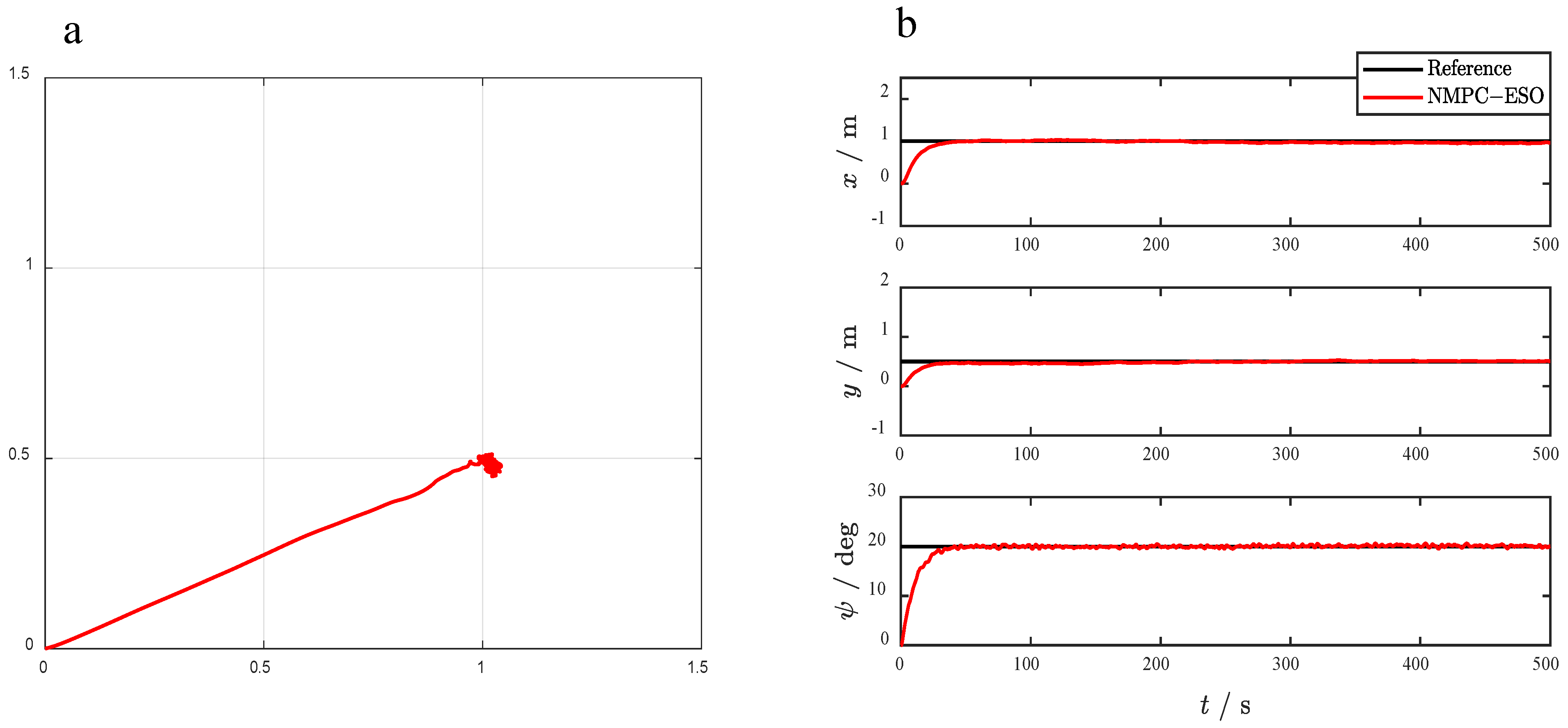
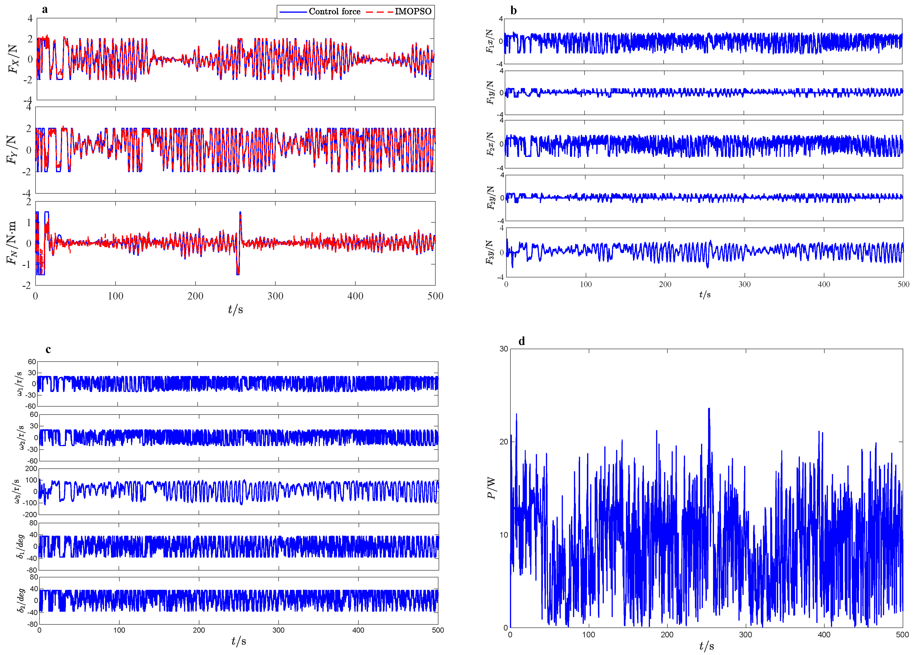
4.2.2. Closed-Loop Control and Thrust Allocation Performance

To further verify the effectiveness of the proposed IMOPSO thrust allocation algorithm in the DP control system, a closed-loop motion control and TA system is established for CSII ship. The schematic diagram is shown in Figure 6. In the DP control system, the simulation model of CSII ship is built based on the mathematical model presented in Equation (7), the ESO is adopted to estimate the unknown disturbances, and the NMPC is used to determine the generalized control force ${\mathit{\tau }}_c$ [34]. Thus, the IMOPSO thrust allocation algorithm is applied to determine the optimal thruster inputs of the propeller speed $\mathit{\omega }$ and the rudder angle $\mathit{\delta }$ to combine the demanded control force. From the DP ship mathematical model (7), we obtain

$$\begin{array}{cc}\hfill \ddot{\mathit{\eta }}& =\mathit{R}\left(\psi \right)\dot{\mathit{\nu }}+\dot{\mathit{R}}\left(\psi \right)\mathit{\nu }\hfill \\ \hfill & =\mathit{R}\left(\psi \right){\mathit{M}}^{-1}(-\mathit{D}\mathit{\nu }+\mathit{d})+\dot{\mathit{R}}\left(\psi \right)\mathit{\nu }+\mathit{R}\left(\psi \right){\mathit{M}}^{-1}{\mathit{\tau }}_c\hfill \end{array}$$

(30)

let $\mathbf{{\rm Y}}=\mathit{R}\left(\psi \right){\mathit{M}}^{-1}(-\mathit{D}\mathit{\nu }+\mathit{d})+\dot{\mathit{R}}\left(\psi \right)\mathit{\nu }$, $\mathbf{\Psi }=\mathit{R}\left(\psi \right){\mathit{M}}^{-1}$ Therefore, (30) is rewritten as

$$\begin{array}{c}\hfill \ddot{\mathit{\eta }}=\mathbf{{\rm Y}}+\mathbf{\Psi }{\mathit{\tau }}_c\end{array}$$

(31)

Remark 2. 

In contrast to the conventional approach of distinguishing between internal and external disturbances in the ship model, Υ is treated as a composite of internal and external disturbances when ESO estimation is employed [35].

From (31), the ship motion model becomes an integral series type system. Let ${\mathit{x}}_1=\mathit{\eta }$, ${\mathit{x}}_2=\dot{\mathit{\eta }}$ and design the ESO as follows:

$$\begin{array}{cc}\hfill & \left\{\begin{array}{cc}\hfill {\dot{\widehat{\mathit{x}}}}_1& ={\widehat{\mathit{x}}}_2+{\mathit{\beta }}_1({\mathit{x}}_1-{\widehat{\mathit{x}}}_1)\hfill \\ \hfill {\dot{\widehat{\mathit{x}}}}_2& ={\widehat{\mathit{x}}}_3+\mathbf{\Psi }{\mathit{\tau }}_c+{\mathit{\beta }}_2({\mathit{x}}_1-{\widehat{\mathit{x}}}_1)\hfill \\ \hfill {\dot{\widehat{\mathit{x}}}}_3& ={\mathit{\beta }}_3({\mathit{x}}_1-{\widehat{\mathit{x}}}_1)\hfill \end{array}\right.\hfill \end{array}$$

(32)

where ${\widehat{\mathit{x}}}_1$ is the observed value of $\mathit{\eta }$, ${\widehat{\mathit{x}}}_2$ is the observed value of $\dot{\mathit{\eta }}$, ${\widehat{\mathit{x}}}_3$ is the observed value of $\mathbf{{\rm Y}}$, and ${\mathit{\beta }}_i,i\in [1,2,3]$ is a constant-valued diagonal matrix.

The optimal control problem for NMPC can thus be formulated as

$$\begin{array}{cc}\hfill & {\displaystyle \underset{\begin{array}{c}\mathit{U}\left(k\right)\end{array}}{min}}\mathit{J}\left(k\right)={\displaystyle \sum _{\begin{array}{c}i=0\end{array}}^{N_p}}(\parallel \widehat{\mathit{\eta }}(k+i|k)-{\mathit{\eta }}_r{\parallel }_{{\mathit{Q}}_c}^2)+{\displaystyle \sum _{\begin{array}{c}i=0\end{array}}^{N_c-1}}{(\parallel \mathit{u}(k+i|k)\parallel }_{{\mathit{R}}_c}^2)\hfill \end{array}$$

(33)

where ${\mathit{N}}_p=50$ is the prediction horizon; ${\mathit{N}}_c=10$ is the control horizon; $\widehat{\mathit{\eta }}$ is the observed value of $\mathit{\eta }$; and ${\mathit{Q}}_c=diag[{10}^2,{10}^2,{10}^2]$, ${\mathit{R}}_c=diag[1,1,1]$ are both positive definite weighted matrices. $\mathit{U}$ represents the control constraint set of the system. To simplify the study, the ship’s oscillatory motions caused by wave-frequency disturbances are not considered in this simulation, and the low-frequency environmental loads acting on the ship are simulated with the first-order Markov process [36]: $\dot{\mathit{d}}=-{\mathit{T}}_{\mathit{c}}^{-\mathbf{1}}\mathit{d}+\rho \mathit{n}$, where ${\mathit{T}}_c=diag(100,100,100)$ is the diagonal matrix of time constants, $\mathit{n}$ is a zero-mean Gaussian white noise vector, and $\rho =diag(0.25,0.25,0.1)$ is the amplitude matrix of $\mathit{n}$. The simulation conditions are set as follows: the initial position of DP ship ${\mathit{\eta }}_0={[0\mathrm{m},0\mathrm{m},0\mathrm{deg}]}^T$; the desired position of the ship ${\mathit{\eta }}_d={[1\mathrm{m},0.5\mathrm{m},20\mathrm{deg}]}^T$; and in order to achieve smooth control, the reference signal is set as ${\mathit{\eta }}_r=\frac{1}{10s+1}{\mathit{\eta }}_d$. The simulation time is set to 500 s.

From the simulation results shown in Figure 7a,b, it can be seen that the DP ship can accurately track the preset $(\mathit{x},\mathit{y})$ position and the yaw angle $\mathit{\psi }$. The results illustrate two folds. On one hand, the NMPC controller performs well; on the other hand, the IMOPSO thrust allocation algorithm can accurately allocate the generalized control force to each thruster with smaller allocation errors.

Figure 8 shows the thrust allocation results of the IMOPSO algorithm under closed-loop control. Figure 8a shows that the IMOPSO algorithm is able to track the generalized control force determined by the NMPC controller. Figure 8b shows the decomposition force generated by individual thruster. Figure 8c shows the change in rotational speed and rudder angle of each thruster. Figure 8d shows the variation in the total power consumption of the thruster. These results further demonstrate that the IMOPSO thrust algorithm performs well in accordance with the motion controller, which verifies the effectiveness of IMOPSO algorithm when dealing with the DP thrust allocation problem.

5. Conclusions

In this paper, an IMOPSO algorithm is proposed for DP ship thrust allocation in a multi-objective optimization perspective. The multiple-objective functions of TA is built, taking into account the allocation objectives of minimizing the allocation error, the power consumption, and the tear-and-wear of thruster system simultaneously. This is different from most studies, which adopt the thrusts and angles as the decision variables herein. Considering the existence of thruster physical constraints, e.g., the saturation constraints on rotational speed and rudder angle, the TA problem may be non-convex; thus, the evolutionary IMOPSO algorithm is specially derived to solve the problem. The IMOPSO algorithm introduces the mechanism of crowding distance and roulette wheel to select the globally optimal particles, and utilizes the local optimization capability. Benchmark comparisons for ZDT1 to ZDT4 functions verify the superiority of IMOPSO on convergence speed and population diversity. Open-loop thrust allocation and closed-loop control simulation are conducted for a propeller–rudder combination DP ship. Simulation results illustrate that, compared with the traditional single-objective PSO thrust allocation method, the proposed IMOPSO thrust allocation algorithm reduces thrust allocation errors in the three directions of surge, sway, and yaw by 48.48%, 39.64%, and 15.02%, respectively, and decreases power consumption by 44.53%. This demonstrates the feasibility and effectiveness of the IMOPSO algorithm in DP ship thrust allocation.

This paper primarily validates the simulation process without applying it to practical experiments, which constitutes a limitation of this study. Future research should focus on several key aspects. Firstly, we consider actual ship experiments and develop an adaptive MOPSO algorithm that can adjust thrust allocation strategies in real-time based on the ship’s operating characteristics under different sea conditions, wind speeds, and loads to ensure safe and efficient operation. Secondly, we consider exploring how to effectively integrate the MOPSO algorithm to achieve optimal coordination among multiple propellers in a system, thus improving the ship’s maneuvering performance and energy efficiency. Additionally, the stability and reliability of the algorithm in long-term operation should be carefully examined through long-term experiments and simulation analyses to evaluate its robustness and durability.

References

1. Zhang, L.; Peng, X.; Wei, N.; Liu, Z.; Liu, C.; Wang, F. A thrust allocation method for DP vessels equipped with rudders. Ocean Eng. 2023, 285, 115342. [Google Scholar] [CrossRef]
2. Bui, T.M.; Dinh, T.Q.; Marco, J.; Watts, C. Development and real-time performance evaluation of energy management strategy for a dynamic positioning hybrid electric marine vessel. Electronics 2021, 10, 1280. [Google Scholar] [CrossRef]
3. Witkowska, A.; Śmierzchalski, R. Adaptive dynamic control allocation for dynamic positioning of marine vessel based on backstep** method and sequential quadratic programming. Ocean Eng. 2018, 163, 570–582. [Google Scholar] [CrossRef]
4. Liu, C.; Zhang, Y.; Gu, M.; Zhang, L.; Teng, Y.; Tian, F. Experimental Study on Adaptive Backstep** Synchronous following Control and Thrust Allocation for a Dynamic Positioning Vessel. J. Mar. Sci. Eng. 2024, 12, 203. [Google Scholar] [CrossRef]
5. Zalewski, P. Convex optimization of thrust allocation in a dynamic positioning simulation system. Zesz. Nauk. Akad. Morskiej Szczecinie 2016, 48, 58–62. [Google Scholar] [CrossRef]
6. Koschorrek, P.; Hahn, T.; Jeinsch, T. A thrust allocation algorithm considering dynamic positioning and roll dam** thrust demands using multi-step quadratic programming. IFAC-PapersOnLine 2018, 51, 438–443. [Google Scholar] [CrossRef]
7. Zalewski, P. Constraints in allocation of thrusters in a dp simulator. Zesz. Nauk. Akad. Morskiej Szczecinie 2017, 52, 45–50. [Google Scholar]
8. Fossen, T.I.; Sagatun, S.I. Adaptive control of nonlinear systems: A case study of underwater robotic systems. J. Robot. Syst. 1991, 8, 393–412. [Google Scholar] [CrossRef]
9. Johansen, T.A.; Fossen, T.I.; Tøndel, P. Efficient optimal constrained control allocation via multiparametric programming. J. Guid. Control Dyn. 2005, 28, 506–515. [Google Scholar] [CrossRef]
10. Sørdalen, O.J. Optimal thrust allocation for marine vessels. Control. Eng. Pract. 1997, 5, 1223–1231. [Google Scholar] [CrossRef]
11. Liang, C.C.; Cheng, W.H. The optimum control of thruster system for dynamically positioned vessels. Ocean. Eng. 2004, 31, 97–110. [Google Scholar] [CrossRef]
12. De Wit, C. Optimal Thrust Allocation Methods for Dynamic Positioning of Ships. Master’s Thesis, Delft Institute of Applied Mathematics, Delft, The Netherlands, 2009. [Google Scholar]
13. Chen, X.; Liu, B.; Le, G. A Multi-Objective Optimization of the Anchor-Last Deployment of the Marine Submersible Buoy System Based on the Particle Swarm Optimization Algorithm. J. Mar. Sci. Eng. 2023, 11, 1305. [Google Scholar] [CrossRef]
14. Yang, J.; Zou, J.; Yang, S.; Hu, Y.; Zheng, J.; Liu, Y. A particle swarm algorithm based on the dual search strategy for dynamic multi-objective optimization. Swarm Evol. Comput. 2023, 83, 101385. [Google Scholar] [CrossRef]
15. Wu, D.; Ren, F.; Zhang, W. An energy optimal thrust allocation method for the marine dynamic positioning system based on adaptive hybrid artificial bee colony algorithm. Ocean. Eng. 2016, 118, 216–226. [Google Scholar] [CrossRef]
16. Guangchi, X.; Dawei, Z.; Kaiwei, Z. Multi-agent chaos particle swarm optimization algorithm of thrust allocation for dynamic positioning vessels. In Proceedings of the 2015 34th Chinese Control Conference (CCC), Hangzhou, China, 28–30 July 2015. [Google Scholar]
17. Yan, H. Research on Optimization Algorithm of the Thrust Allocation for Dynamic Positioning Systems of ships. Master’s Thesis, Dalian Maritime University, Dalian, China, 2011. [Google Scholar]
18. Ji, M.; Yi, B. The optimal thrust allocation based on QPSO algorithm for dynamic positioning vessels. In Proceedings of the 2014 IEEE International Conference on Mechatronics and Automation, Beijing, China, 2–5 August 2014. [Google Scholar]
19. Coello, C.A.C.; Pulido, G.T.; Lechuga, M.S. Handling multiple objectives with particle swarm optimization. IEEE Trans. Evol. Comput. 2004, 8, 256–279. [Google Scholar] [CrossRef]
20. Zhao, J.; Li, Y.; Bai, J.; Ma, L.; Shi, C.; Zhang, G.; Shi, J. Multi-objective optimization of marine nuclear power secondary circuit system based on improved multi-objective particle swarm optimization algorithm. Prog. Nucl. Energy 2023, 161, 104740. [Google Scholar] [CrossRef]
21. Mou, J.; Zhu, Q.; Liu, Y.; Bai, Y. Multi-objective optimal thrust allocation strategy for automatic berthing of surface ships using adaptive non-dominated sorting genetic algorithm III. Ocean. Eng. 2024, 299, 117288. [Google Scholar] [CrossRef]
22. Xuebin, L. Dynamic multiobjective optimization for thrust allocation in ship application. Ocean. Eng. 2020, 218, 108187. [Google Scholar] [CrossRef]
23. Nasouri, M.; Bidhendi, G.N.; Hoveidi, H.; Amiri, M.J. Parametric study and performance-based multi-criteria optimization of the indirect-expansion solar-assisted heat pump through the integration of Analytic Network process decision-making with MOPSO algorithm. Sol. Energy 2021, 225, 814–830. [Google Scholar] [CrossRef]
24. Li, G.; Zhou, T. A multi-objective particle swarm optimizer based on reference point for multimodal multi-objective optimization. Eng. Appl. Artif. Intell. 2022, 107, 104523. [Google Scholar] [CrossRef]
25. Li, Y.; Lei, J. A feasible solution to the beam-angle-optimization problem in radiotherapy planning with a DNA-based genetic algorithm. IEEE Trans. Biomed. Eng. 2009, 57, 499–508. [Google Scholar] [PubMed]
26. Wang, Y.; Cheng, H.; Wang, C.; Hu, Z.; Yao, L.; Ma, Z.; Zhu, Z. Pareto optimality-based multi-objective transmission planning considering transmission congestion. Electr. Power Syst. Res. 2008, 78, 1619–1626. [Google Scholar] [CrossRef]
27. Fossen, T.I. Handbook of Marine Craft Hydrodynamics and Motion Control, 1st ed.; Wiley: Hoboken, NJ, USA, 2011. [Google Scholar]
28. Deng, F.; Zhang, H.; Ding, Q.; Zhang, S.; Du, Z.; Yang, H. PSO and NNPC-based integrative control allocation for dynamic positioning ships with thruster constraints. Ocean. Eng. 2024, 292, 116553. [Google Scholar] [CrossRef]
29. Johansen, T.A.; Fossen, T.I.; Berge, S.P. Constrained nonlinear control allocation with singularity avoidance using sequential quadratic programming. IEEE Trans. Control. Syst. Technol. 2004, 12, 211–216. [Google Scholar] [CrossRef]
30. Eberhart, R.; Kennedy, J. Particle swarm optimization. In Proceedings of the IEEE International Conference on Neural Networks, Perth, WA, Australia, 27 November–1 December 1995. [Google Scholar]
31. Deb, K.; Pratap, A.; Agarwal, S.; Meyarivan, T.A.M.T. A fast and elitist multiobjective genetic algorithm: NSGA-II. IEEE Trans. Evol. Comput. 2002, 6, 182–197. [Google Scholar] [CrossRef]
32. Zapotecas Martínez, S.; Coello Coello, C.A. A multi-objective particle swarm optimizer based on decomposition. In Proceedings of the 13th Annual Conference on Genetic and Evolutionary Computation, Dublin, Ireland, 12–16 July 2011. [Google Scholar]
33. Lindegaard, K.P.; Fossen, T.I. Fuel-efficient rudder and propeller control allocation for marine craft: Experiments with a model ship. IEEE Trans. Control. Syst. Technol. 2003, 11, 850–862. [Google Scholar] [CrossRef]
34. Deng, F.; Yang, H.L.; Wang, L.J.; Yang, W.M. UKF based nonlinear offset-free model predictive control for ship dynamic positioning under stochastic disturbances. Int. J. Control. Autom. Syst. 2019, 17, 3079–3090. [Google Scholar] [CrossRef]
35. Zhang, Q.; Guo, C. Anti-disturbance lyapunov-based model predictive control for trajectory tracking of dynamically positioned ships. J. Mar. Sci. Eng. 2023, 11, 281. [Google Scholar] [CrossRef]
36. Tang, L.; Liu, J.; Wang, L.; Wang, Y. Robust fixed-time trajectory tracking control of the dynamic positioning ship with actuator saturation. Ocean. Eng. 2023, 284, 115199. [Google Scholar] [CrossRef]
Figure 1. Path of the particle update.
Jmse 12 01118 g001
Figure 2. Inertia weight updating methods.
Jmse 12 01118 g002
Figure 3. IMOPSO test results for ZDT1 to ZDT4 functions.
Jmse 12 01118 g003
Figure 4. Thrust configuration for CSII.
Jmse 12 01118 g004
Figure 5. The simulation results of thrust allocation 1: (a) The total generalized forces of the thruster system. (b) The generalized force generated by each thruster. (c) Allocated propeller speed and rudder angle of each thruster. (d) Total thruster power consumption.
Jmse 12 01118 g005
Figure 6. Principle of DP closed-loop control system.
Jmse 12 01118 g006
Figure 7. The simulation results of closed-loop DP control: (a) Ship’s trajectory. (b) Position and bow angle of the ship.
Jmse 12 01118 g007
Figure 8. The simulation results of closed-loop thrust allocation: (a) The total generalized forces of the thruster system. (b) The generalized force generated by each thruster. (c) Allocated propeller speed and rudder angle of each thruster. (d) Total thruster power consumption.
Jmse 12 01118 g008