Article

Reinforcement-Learning-Based Visual Servoing of Underwater Vehicle Dual-Manipulator System

by
Yingxiang Wang
and
Jian Gao
*
School of Marine Science and Technology, Northwestern Polytechnical University, Xi’an 710072, China
*
Author to whom correspondence should be addressed.
J. Mar. Sci. Eng. 2024, 12(6), 940; https://doi.org/10.3390/jmse12060940
Submission received: 21 April 2024 / Revised: 28 May 2024 / Accepted: 1 June 2024 / Published: 3 June 2024
(This article belongs to the Section Ocean Engineering)

Abstract

:
As a substitute for human arms, underwater vehicle dual-manipulator systems (UVDMSs) have attracted the interest of global researchers. Visual servoing is an important tool for the positioning and tracking control of UVDMSs. In this paper, a reinforcement-learning-based adaptive control strategy for the UVDMS visual servo, considering the model uncertainties, is proposed. Initially, the kinematic control is designed by developing a hybrid visual servo approach using the information from multi-cameras. The command velocity of the whole system is produced through a task priority method. Then, the reinforcement-learning-based velocity tracking control is developed with a dynamic inversion approach. The hybrid visual servoing uses sensors equipped with UVDMSs while requiring fewer image features. Model uncertainties of the coupled nonlinear system are compensated by the actor–critic neural network for better control performances. Moreover, the stability analysis using the Lyapunov theory proves that the system error is ultimately uniformly bounded (UUB). At last, the simulation shows that the proposed control strategy performs well in the task of dynamical positioning.

1. Introduction

Unmanned underwater vehicles (UUVs) play an important role in the exploration of oceans. With the increasing demand for ocean development, the UUV, lacking the intervention ability, is no longer capable of handling certain tasks [1]. Meanwhile, the underwater vehicle manipulator system (UVMS) has been widely used in the marine energy and underwater architecture industry, and significant results have been achieved [2,3]. The application scenarios of the UVMS include but are not limited to, underwater pipeline inspection [4], ship maintenance [5], underwater rescue [6], terrain exploration [7], marine biology research [8,9], and marine archaeology research [10,11].
At present, these industrial UVMS are often fixed on the seabed during operation, forming a stable working environment, which ensures a certain level of security and sustained stable output while the scope and flexibility are limited. Furthermore, many underwater tasks cannot provide a reliable ground support environment. This makes it necessary to develop the floating-based UVMS, especially for the scenes of the bridge and the pipeline maintenance that require continuous movement, as well as the scenes such as marine archaeology and biological research that need to avoid damage to the environment during the operation. Based on UVMSs, underwater vehicle dual-manipulator systems (UVDMSs) have received a lot of research attention in recent years.
In terms of UVMS, the Girona 500 UVMS [12] of Girona University has dealt with tasks such as dynamic positioning and object grasping. The Dexrov project [13] has reduced the dependence on the work environment with the concept of remote operation. The Ocean One project [14,15] of Stanford University has developed a dual-arm humanoid robot with strong operational capabilities and perception capabilities. By remote operation, it has successfully carried out an archaeological task. Ref. [16] studied the task of moving an object to a precisely positioned peg while considering the impacts due to contact and provided a multiple impedance manipulation method that exhibits a smooth performance in the simulation. A whole-body control strategy of UVDMSs proposed in the MARIS Italian research project [17] has extended the task priority framework to deal with coordination manipulation and transportation problems. An alternative dual-arm configuration of UVDMSs is designed in [18] with only one manipulator for task operation and another for pose maintenance. This unique concept is proven to perform well in the presence of currents. Ref. [19] recently showed another different style of UVDMS similar to an underwater glider and provided a moving strategy making use of drag, which provides a low-power consumption solution for UVDMSs.
All the applications and research of the UVDMS above require reliable control methods, and the primary objective of the UVMS control is the dynamic positioning that ensures a stable working environment for other tasks. Due to the limitations of underwater signal transmission, visual positioning is commonly used for operations in the local space. The most widely used visual servo method is the image-based visual servo (IBVS) [20,21], which does not require calculating the 3D information of the targets. Refs. [22,23] propose a visual servo strategy for dynamic positioning, which utilizes the measuring sensors equipped with the UUV and achieves significant results. In [24], the visual servo method has been applied to the UVMS system, while the redundancy problem is solved through model prediction, resulting in a good positioning performance. However, few studies focus on visual positioning for the UVDMS. Considering that the manipulators of the UVDMS are usually installed away from the vehicle center, unlike the UVMS, in which the manipulator is always fixed along the center of gravity and buoyancy. This configuration has a significant impact on the stability of the system, and greater torques are required during the positioning task. Additionally, dual manipulators bring more difficulties for motion planning since the joint limits and collision risks increase.
Modeling the UVMS dynamics is challenging, as it requires consideration of both the impact of the water and coupling effects between the manipulators and the vehicle. A brief description of the kinematic and dynamic models of the UVMS is provided in [25]. Considering the model in [25], the numerical simulation is executed for the dynamic model in [26], and the coupling between the dual manipulators and the vehicle is analyzed in this work. It is impossible to develop a mathematical model that accurately represents the physical system. Until now, control research of the UVMS mostly uses robust and adaptive tools to solve the model uncertainties. In [24], the model coupling information is estimated by the EKF filter, and the model predictive-based control provides an optimal kinematic solution. In [27], the sliding mode control of the UVMS, with certain anti-interference ability, has been provided for a tracking task. To deal with uncertainties and disturbance, Refs. [28,29] provide the adaptive control strategy and observer-based method, respectively, and both of them show good performance while handling uncertainties.
Based on the research above, this work studies the visual servo control of the UVDMS, considering the model uncertainties. A hybrid visual servo method is proposed based on the multiple cameras and attitude sensors equipped with the UVDMS. The command velocity is produced by the kinematic controller using the task priority scheme. In addition, the reinforcement-learning-based speed tracking controller was designed, and the system model error is compensated by the designed actor neural network. Meanwhile, the error system is proved to be ultimately uniformly bounded by the Lyapunov method. Finally, a UVDMS model is simulated, and the results prove the effectiveness of the proposed control.
This paper is organized as follows. Section 2 describes the mathematical model of the kinematics and dynamics of the UVDMS, as well as the hybrid visual servo model of the UVDMS. Section 3 formulates the kinematic control that produces the command velocity to be tracked. In Section 3, the reinforcement-learning-based adaptive control is formulated, while the actor–critic networks are designed to compensate for the system uncertainties. And the stability analysis is down in this section. Then, the simulation work using an 18-dof UVDMS is shown in Section 4. At last, in Section 5, a brief summary of this work is provided.

2. Problem Formulation

This section introduces the kinematics and dynamics of the UVDMS by providing the necessary coordinates and variables. A visual servo model considering the camera configuration of the UVDMS is established. In addition, a task priority strategy for redundancy control and a universal reinforcement learning method based on the actor–critic algorithm are provided. At last, the objective of this study is described.

2.1. UVMS Model

To illustrate the modeling of UVDMS, a 3D model consisting of a fully actuated UUV and two 6-dof manipulators is shown in Figure 1. Obviously, this is a redundant system with 18 degrees of freedom. According to [25,30], the underwater rigid body model can be described in several coordinate frames defined as Σ i  (the inertial frame), Σ b  (the vehicle body fixed frame with origin at the center of the mass), Σ c  (the main camera frame), Σ 0 i (the manipulator base frame, i = 1 , 2 ), Σ c i (the camera frame fixed with the end effector, i = 1 , 2 ), and Σ e i (the end-effector frame attached at the end of the manipulator, i = 1 , 2 ). In frame Σ i , the pose vector of the base vehicle is defined as η = [ x , y , z , φ , θ , ψ ] T , which contains the global position η 1 = [ x , y , z ] T and Euler angles η 2 = [ φ , θ , ψ ] T . The vehicle’s velocity v = [ u , v , w , p , q , r ] T containing the linear velocity v 1 = [ u , v , w ] T and the angular velocity v 2 = [ p , q , r ] T is defined in frame Σ b .
In terms of the underwater manipulators, the states are generally described as the joint angles q = [ q l , q r ] T , with q l = [ q i 1 , q i 2 , q i 3 , q i 4 , q i 5 , q i 6 ] T , and the corresponding velocity q ˙ = [ q ˙ l , q ˙ r ] T , with q ˙ i = [ q ˙ i 1 , q ˙ i 2 , q ˙ i 3 , q ˙ i 4 , q ˙ i 5 , q ˙ i 6 ] T , where i = l , r . Combining both the velocities of the UUV and the manipulators, one obtains the motion transformation from the vehicle body frame to the inertial frame as
[ η ˙ 1 η ˙ 2 q ˙ ] = [ R B I 0 3 0 3 × 12 0 3 J k , o 1 ( η ) 0 3 × 12 0 12 × 3 0 12 × 3 I 12 ] ζ = J k 1 ζ , ζ = [ v 1 v 2 q ˙ ] 18 × 1 ,
where R B I 3 × 3 is the rotation matrix from the vehicle body frame to the inertial frame, and J k , o 1 ( η ) 3 × 3 is the Jacobian matrix of the vehicle angular velocity. Then, the relationship between the system velocity and the end effector velocity can be formulated as
η ˙ e e = [ η ˙ e e , 1 η ˙ e e , 2 ] = J ( R B I , q ) ζ = [ J 1 ( R B I , q ) J 2 ( R B I , q ) ] ζ .
The equation above is a brief description of the direct kinematic of the UVMS with the Jacobian J 18 × 18 including J 1 6 × 18 (Jacobian of the left end effector) and J 2 6 × 18 (Jacobian of the right end effector), which can be computed by the DH parameters and the rotation matrix. η e e , 1 = [ x e 1 , y e 1 , z e 1 , φ e 1 , θ e 1 , ψ e 1 ] T and η e e , 2 = [ x e 2 , y e 2 , z e 2 , φ e 2 , θ e 2 , ψ e 2 ] T present poses of the left and right end effectors respectively.
Most of the system uncertainties come from the UVDMS dynamics since it is difficult to obtain the hydrodynamic and internal couplings precisely. For simplicity, this work formulates a concise Lagrangian dynamic model without considering the water velocity as follows:
M ( q ) ζ ˙ + C ( q , ζ ) ζ + D ( q , ζ ) ζ + g ( q , η 2 ) = τ ,
where M ( q ) 18 × 18 represents the inertial matrix consisting of both the vehicle’s inertia and the manipulators’ inertia on the diagonal, while other matrix elements represent the coupling factors. Similarly, the added Coriolis and centripetal matrix C ( q , ζ ) 18 × 18 is developed in a compact manner, as well as the damping and hydrodynamic lift matrix D ( q , ζ ) 18 × 18 . τ = [ τ v , τ q ] T and g ( q , η 2 ) denote the input vector of the vehicle and joint torques and the restoring forces by gravity buoyancy, respectively. As a rigid body system, these matrices have the following properties: the symmetric matrix M ( q ) is positively defined with m 1 ( q ) M ( q ) m 2 ( q ) , where m 1 and m 2 are positive definite functions, and C ( q , ζ ) can be chosen to satisfy x T ( M ˙ 2 C ) x = 0 . The dynamic model can be written as a general nonlinear differential equation ζ ˙ = f ( τ , ζ , q , η 2 ) to simplify the subsequent derivation.

2.2. Visual Servo Model

Traditional image-based visual servo requires multiple feature points or specially shaped patterns, which are not easy to obtain or deploy underwater. Fortunately, the UUVs, especially the UVMS, are always equipped with several cameras so that fewer feature points are needed by developing a semi-stereoscopic visual system.
In this work, we consider that the UVDMS has two cameras fixed with both end effectors and a main camera fixed with the vehicle body. As long as the object feature (i.e., a single point) is within all the cameras’ field of view, the depth information can be computed by taking advantage of the transformation between the hand cameras and the body camera. Then, the visual servo model is formulated briefly to provide a command velocity for the dynamic control.
The transformation from the camera velocity in the camera frame to the image feature velocity in the image plane is described as
s ˙ = L ( s , z ) v c ,
where
L ( s , z ) = [ ρ m z 0 m z m n ρ n ρ m 2 + m 2 ρ m ρ m n ρ n 0 ρ n z n z ρ n 2 + n 2 ρ m m n ρ m ρ n m ρ m ] .
This equation shows that the feature point s = ( m , n ) in the image plane is driven by the camera velocity v c with the image Jacobian L ( s , z ) 2 × 6 . The scalar variable z , z-position of the object in the camera frame, will be calculated with the Jacobian of the main camera and the camera’s internal parameters in L are obtained by camera calibration. To make full use of the sensors on the UUV (i.e. IMU), an augmented feature vector (including the image features, the image depth, and the Euler angles of the end effector) and its desired form are defined as
χ 1 = [ m e 1 , n e 1 , z e 1 , ϕ e 1 , θ e 1 , ψ e 1 ] T , χ 1 = [ m e 1 , n e 1 , z e 1 , ϕ e 1 , θ e 1 , ψ e 1 ] T .

3. Control Strategy Developments

3.1. Hybrid Visual Servo

Without loss of generality, the left manipulator is taken as an example, and it is assumed that the camera frame is fixed with the end effector frame with no translation and rotation (shown in Figure 1). By transforming the object position [xe1,ye1,ze1]T  into the end effector frame, the homogeneous transformation is formulated to obtain z 0 .
[ x c 1 y c 1 z c 1 ] = T 0 1 C T e 1 0 1 ( q l ) ( [ x e 1 y e 1 z e 1 ] ) .
With the image Jacobians L c 1 and L e 1 defined above, z e 1 can be calculated by the scalar function z e 1 ( m e 1 , n e 1 , m c 1 , n c 1 , q l ) . At the same time, we can obtain [ φ e 1 , θ e 1 , ψ e 1 ] T using the equation [ φ e 1 , θ e 1 , ψ e 1 ] T = R I e 1 ( R B I , q l ) [ φ , θ , ψ ] T , where R I e 1 is the rotation matrix from the inertial frame to the left end effector frame. Thus, the augmented visual servo model is developed as
χ ˙ 1 = [ L ( s , z e 1 ) R I e 1 ( η e e 2 , 1 ) 3 0 1 × 3 0 3 × 3 J k , o 1 ( η e e 2 , 1 ) ] η ˙ e e , 1 = J χ 1 η ˙ e e , 1 .
where η e e 2 , 1 is the orientation of the left end effector, R I e 1 3 represents the third component of R I e 1 , and J k , o 1 is the Jacobian from the inertial frame to the let end effector frame. Combining Equation (8) with Equation (2), together with the right manipulator visual servo model χ ˙ 2 = J χ 2 η ˙ e e , 2 and the combined image feature error e s = χ χ , one has the transformation from the system velocity to the image error change rate.
e ˙ s = χ ˙ = [ χ ˙ 1 χ ˙ 2 ] = [ J χ 1 0 6 × 6 0 6 × 6 J χ 2 ] [ η ˙ e e , 1 η ˙ e e , 2 ] = J χ J ζ = J v s ζ .
A candidate desired velocity can be chosen as ζ d = λ J v s + e s to drive the feature points converge to the target point exponentially, where J v s + = ( J v s T J v s ) 1 J v s T 18 × 12 is the pseudo-inverse Jacobian matrix and λ is a positively defined diagonal matrix. In terms of a single UUV, this velocity command is sufficient for a positioning task. However, directly using the command velocity of IBVS will not stabilize the UVDMS system for its high redundancy and coupling characteristic. The task priority solution is an effective way to deal with system redundancy by decoupling the UVDMS motions as several tasks. As the end effector visual servo model contains the image depth and Euler angles in the closed loop, that means the position and orientation of the end effector are already configured. Using the remaining freedoms for the positioning of the UUV body can solve the redundancy problem. Then, a similar formulation for the vehicle body is given by e ˙ b = χ ˙ b = J b ζ b , where e b = χ b χ b is the UUV image error and χ b = [ m b , n b , z b , φ , θ , ψ ] T is the augmented image features (with the vehicle Euler angles and the image depth) of the target obtained by the camera at the bottom of the vehicle. χ b = [ m b , n b , z b , φ , θ , ψ ] T is the desired UUV target image feature and J b 6 × 18 is the Jacobian of the vehicle positioning. Similarly, the desired velocity for UUV positioning is defined as ζ b d = λ J b + e b . It should be pointed out that z b is measured by the depth sensor (i.e., the DVL or laser sensors) instead of computing. Thus, the command velocity is described as follows.
ζ c m d = J v s + ζ d + ( I 18 × 18 J v s + J v s ) J b + ζ b d J v s + = W 1 J v s T ( J v s W 1 J v s T ) 1 J b + = W 1 J b T ( J b W 1 J b T ) 1 ,
In this equation, the pseudo-inverse of both Jacobian matrices is modified by a weight matrix to avoid joint limits, and the operation above projects the desired vehicle velocity onto the zero space of J v s as the secondary task so that the manipulator visual servo will not be affected. The command velocity will be tracked by the control method proved in the next section.

3.2. Velocity Tracking Control

As it is hard to obtain the exact dynamics of the UVDMS, the control of this kind of strong nonlinear coupled system is challenging. To achieve a good control performance, an adaptive control scheme, shown in Figure 2, is proposed to deal with the system uncertainties.
Given the measured system elements M ¯ ( q ) , C ¯ ( q , ζ ) , D ¯ ( q , ζ ) ζ ˙ , and g ¯ ( q , η 2 ) , the control law is designed as
M ¯ ( q ) a + C ¯ ( q , ζ ) ζ + D ¯ ( q , ζ ) ζ + g ¯ ( q , η 2 ) = τ ,
where a is regarded as the virtual control to be designed later. Multiplying by M ¯ 1 ( q ) on each side of the equation, we obtain
a = M ¯ 1 ( q ) τ C ¯ ( q , ζ ) ζ D ¯ ( q , ζ ) ζ g ¯ ( q , η 2 ) = f ¯ ( τ , ζ , q , η 2 ) .
By defining the model error as Δ ( τ , ζ , q , η 2 ) = f ( τ , ζ , q , η 2 ) f ¯ ( τ , ζ , q , η 2 ) , the dynamic system can be written as the feedback linearization form
ζ ˙ = a + Δ ( τ , ζ , q , η 2 ) .
It can be seen that a properly designed a can stabilize the system with compensation for Δ ( τ , ζ , q , η 2 ) . Therefore, the virtual control design is given below using the reference model adaptive strategy.
a = a r m + a l c + a r l ,
where a r m is the dynamic of the first-order reference model a r m = K r m ( ζ c m d ζ r m ) , with K r m being positively defined and ζ r m as the desired tracking velocity with the same initial conditions as the system. The tracking error and its dynamic is defined as
e = [ 0 t ( ζ r m ζ ) d τ ζ r m ζ ] e ˙ = [ ζ r m ζ a r m ζ ˙ ] = [ 0 I K i K p ] e + [ 0 I ] ( a r l Δ ( τ , ζ , q , η 2 ) ) =   Λ e + B ( a r l Δ ( τ , ζ , q , η 2 ) ) ,
where K p and K i are the control parameters from the reference velocity tracking control a l c , and a l c is the compensation signal from the actor neural network.

3.3. Actor–Critic Network

The deterministic policy gradient (DPG) method is introduced to deal with the system uncertainties. Typically, this strategy includes two neural networks, π ( x a , θ ) = θ T φ a ( x a ) + ε a and V c = q ( x v , W ) = W T φ v ( x v ) + ε v , named the actor network and the critic network, respectively. In this work, the actor network aims to compensate Δ ( τ , ζ , q , η 2 ) with x a = [ τ , ζ , q , η 2 ] T as the action with its parameters as the states. On the other hand, the quality of the actor is evaluated by the value function, which is approximated by the critic network. For the continuous dynamic system, the penalty function in an integral form is developed as follows:
V c = t P d τ , P = e T ( t ) Q e ( t ) ,
where Q is a positive definite matrix, and P is regarded as the reward function. The critic network V ^ c ( x v , W ^ ) = W ^ T φ v ( x v ) is used to approximate V c . To avoid the complexity of the process, the variables of the networks are abbreviated later. According to the TD target update strategy [31], a critic error function is formulated as
e v = P ( t ) + V ^ ˙ c ( x v , W ^ ) .
The goal of updating W ^ is to minimize the target error E v = 1 / 2 e v T e v so that the update law based on its gradient is provided in a brief form as
W ^ ˙ = Γ v ( W ^ T φ ˙ v + P ) φ ˙ v β Γ v W ^ ,
where Γ v (the learning rate) and β are positive definite. Similarly, another error function that contains both information of V ^ c and π ^ is described as
e a = ϖ V ^ c + ( θ ^ T θ T ) φ a E a = 1 2 e a T e a .
The actor error E a will reduce as long as V ^ c reduces and θ ^ is close to θ . Then, the update law can be easily derived from the gradient of E a as
θ ^ ˙ = Γ a φ a ( ϖ V ^ c θ ^ T φ a ) T α Γ a θ ^ ,
where α and Γ a have the same definition as the critic network. For further study, the parameters of the neural networks must satisfy
φ a φ m a , φ v φ m v , ε a ε m a , ε v ε m v φ ˙ a φ d m a , φ ˙ v φ d m v , W W m , θ θ m .
Lemma 1. 
Considering the update law given in (18) and (20), the neural network weight errors W ˜ = W ^ W  and   θ ˜ = θ ^ θ  are bounded by the compact sets
Φ v = { W ˜ | W ˜ δ c } Φ a = { θ ˜ | θ ˜ δ a } δ c W m ( φ d m v 2 + φ d m v φ m v ) 2 ( φ d m v 2 + β 1 ) δ a 2 ϖ T ϖ ( δ c 2 + W m 2 ) φ m v 2 + θ m 2 ( φ a m 2 + 1 / 2 α ) φ m a 2 + α .
The proof of Lemma 1 using the assumptions in Equation (21) and the two Lyapunov functions in Equation (23) is similar to that in [32]. This work will directly use this conclusion.
V 1 = tr ( W ˜ T Γ v 1 W ˜ ) V 2 = tr ( θ ˜ T Γ a 1 θ ˜ ) .

3.4. Stability Analysis

By substituting the actor network π ( x a , θ ) = θ T ϕ a ( x a ) + ε a into Equation (15), the error dynamic can be written as
e ˙ = Λ e + B ( π ^ π ε a ) = Λ e + B ( θ ^ T φ a θ T φ a ε a ) = Λ e + B ( θ ˜ T φ a ε a ) = Λ e + Ω θ ˜ = θ ^ θ .
A Lyapunov candidate of the system error can be defined as
V L = 1 2 e T P r e ,
where P r is a positive definite matrix satisfying
Λ T P r + P r Λ = Q r , Q r > 0 .
Then, we obtain the derivative of V L as
V ˙ L = 1 2 e ˙ T P r e + 1 2 e T P r e ˙ = 1 2 e T ( Λ T P r + P Λ ) e + 1 2 Ω T P r e + 1 2 e T P r Ω = 1 2 e T ( Q r ) e + e T P r Ω = 1 2 e T ( Q r ) e + e T P r B θ ˜ φ a e T P r B ε a 1 2 λ min ( Q r ) e 2 + λ max ( P r ) e ( ε m a + δ a ) = 1 2 e ( λ min ( Q r ) e + λ max ( P r ) ( ε m a + δ a ) ) .
In the inequality above, Lemma 1 is used. Then we have V ˙ L 0 when
e 2 λ max ( P r ) ( ε m a + δ a ) λ min ( Q r ) .
This means that e is uniformly ultimately bounded, and the convergence speed depends on the minimum eigenvalue of Q r . Moreover, the more accurate the neural network’s approximations are, the better the velocity-tracking controller performs.

4. Simulation Experiments

This section shows the simulation experiments to test the performance of the proposed visual servo control method for UVDMSs using Matlab R2023b and Unity 2022 The dynamic parameters of the UUV model shown in Figure 1 are listed as follows:
M R B = d i a g { 106 , 106 , 106 , 9.5 , 10.2 , 12 } M A M = d i a g { 63 , 32.2 , 31.3 , 5.6 , 3.7 , 3.4 } D ( v ) = d i a g { 110 + 90 | v | , 90 + 90 | v | , 140 + 110 | v | , 20 + 8 | v | , 13 + 10 | v | , 17 + 12 | v | }
The weight of the vehicle is 106 kg, while the buoyant force is 1058 N. The centers of the gravity and the buoyancy are r G = [ 0 , 0 , 0.1 ] and r B = [ 0 , 0 , 0.1 ] . The manipulator’s geometrical parameters are shown in Figure 3 and Table 1.
Inspired by simurv 4.0 [17], the dynamics of each single rigid body link and the UUV are projected into the generalized velocity coordinates to be added together as the generalized forces of 18 dimensions, which formulates the dynamic model of the UVDMS. Using the Jacobians and DH functions from simurv 4.0, the transformation between different frames can be easily achieved when developing the kinematics. The model parameters of the UUV are computed through Creo 10.0 (designing all models and measuring moment of inertial of the rigid bodies) and Ansys 2019 R3 (Computed Fluid Dynamics module of the Ansys Workbench is used for the identification of UUV hydrodynamic parameters).
η = [ 0.5 , 0.2 , 0.9 , 0 , 0 , 0 ] and q = [ 0 , 30 , 5 , 30 , 0 , 0 , 0 , 30 , 5 , 30 , 0 , 0 ] are the initial conditions of the states. The target coordinates in the inertial frame are t a 1 = [ 1.5 , 0.3 , 3 ] and t a 2 = [ 1.5 , 0.7 , 3 ] . The desired position of the vehicle is η d = [ 1 , 0.5 , 2.6 , 0 , 0 , 0 ] , and the desired orientations of both end effectors are towards the x-direction of the inertial coordinate with their z-axis.
The simulation results of the UVDMS position and orientation are shown in Figure 4, Figure 5, Figure 6 and Figure 7, including the pose of the vehicle in Figure 4, the angles of both manipulators in Figure 5, the position of both end effectors in Figure 6, the orientation(in the form of Euler angles) of both end effectors in Figure 7a. It can be seen that all states tend to be stable eventually. Comparing the convergence time of the vehicle position with that of the end effectors, we see that the vehicle arrived at its target earlier. That is, before the visual servoing, the vehicle should be driven to the working space by changing the task’s priority. The vehicle Euler angles show that the angles of the roll and pitch change more significantly than the yaw angle, which is caused by the floating-based operation with gravity changing during the movement. Similarly, this phenomenon also occurred in the figure of the velocities and torques below since the controller is trying to restore the orientation. In Figure 5, the angles of all joints change smoothly without exceeding the joint limits. In addition, Figure 6 indicates that the task priority strategy results in smoother curves of the end effector than that of the UUV.
The UVDMS velocity are shown in Figure 7b, Figure 8 and Figure 9, where Figure 7b shows the linear velocities of the end effectors, Figure 8 shows the linear and angular velocities of the vehicle, and the angular velocity of all manipulator joints are in Figure 8. From the velocity figures, it can be observed that most velocities are within the limits and running safely. Then, the command torques of the vehicle and manipulators are shown in Figure 10 and Figure 11. It can be seen that the command torques are always working until the simulation stops. That is, during the dynamic positioning, the open loop system is far away from its equilibrium with two manipulators forward. This is also proved by the pitch velocity and y-torque curves, which have larger values than others. The joint torques of both manipulators show that the joints closer to the base require more torques for moving. It should be noted that to compensate for gravity, several torques (joints 2–4) maintain non-zero values in the end.
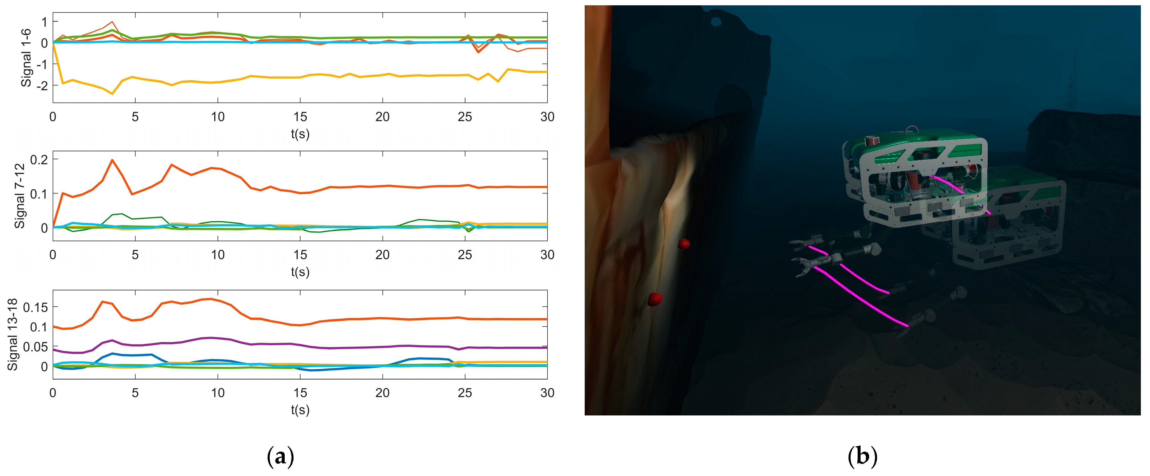
At last, in Figure 12a, the compensation signals, divided into three parts, from the actor neural network are plotted, which indicates the system error (including the disturbance). It is assumed that the system uncertainty is bounded and does not change drastically when the estimated model is close enough to the real system model. So, we use RBF neural networks as the actor and critic networks for their infinite approximation ability and simple configurations. The base functions are Gaussian basis functions with the number of neurons as 100. A direct influence of the actor–critic networks on the control performance is that the parameter adjustment of the linear controller is easier. The simulation data have been displayed in Unity 2022 with the lightweight UVDMS designed by the author to test the control strategy as well as to avoid joint collisions and singularities. As shown in Figure 12b, the UVDMS successfully tracked the target features and positioned itself by the side of the shipwrecks. The purple trajectories show that the vehicle center and both end effectors move smoothly.

5. Conclusions

A reinforcement-learning-based adaptive control for the visual servoing of a UVDMS equipped with two six-dof manipulators is developed in this work: (a) Different from the classical IBVS schemes, the proposed hybrid visual servo takes advantage of the multiple cameras and other sensors to obtain the image depth such that fewer target image features are needed. (b) The command velocity is computed through a kinematic controller using the task priority method, considering both the positioning of the vehicle and the visual servo command. (c) In addition, a DPG strategy is used to design an actor–critic method to deal with the system uncertainties. The model uncertainty is compensated by the actor neural network, while the critic neural network evaluates the performance of the actor. The critic network is updated by the gradient of the velocity tracking error, and the actor is adjusted by the critic network. (d) Also, it is proved that the tracking error of the velocity is ultimately bounded using the Lyapunov method. (e) At last, the simulation of the UVDMS using Matlab and Unity shows a good performance of the proposed strategy.
This approach aims to provide a dynamic positioning method for UVDMSs’ tasks in a relatively stable local environment. However, the effects of currents, joint dynamics, thruster dynamics, low-quality underwater images, unknown environments, and low-precision sensor measurements (especially the linear velocity of UUV) are not taken into account. Additionally, collision avoidance (especially the mutual manipulators’ collision avoidance problem) and cooperative control are not involved.
Control and planning of the UVMS, especially the UVDMS, are challenging. Due to the coupling and uncertainty problems, designing a universal high-performance controller is far more difficult than for manipulators on land or UUVs. At the same time, the demand for ocean exploration makes the research of UVDMS and UVMS promising. Therefore, the follow-up study of this work will continue by focusing on the motion planning and visual control of the UVDMS.

Author Contributions

Conceptualization, Y.W. and J.G.; methodology, Y.W.; software, Y.W.; investigation, Y.W.; resources, J.G; writing—original draft preparation, Y.W.; writing—review and editing, Y.W. and J.G.; visualization, Y.W.; supervision, J.G. All authors have read and agreed to the published version of the manuscript.

Funding

This research was funded by the National Natural Science Foundation of China, grant numbers 51979228 and 52102469.

Institutional Review Board Statement

Not applicable.

Informed Consent Statement

Not applicable.

Data Availability Statement

Data are contained within the article.

Conflicts of Interest

The authors declare no conflicts of interest.

References

  1. Ridao, P.; Carreras, M.; Ribas, D.; Sanz, P.J.; Oliver, G. Intervention AUVs: The next challenge. Annu. Rev. Control 2015, 40, 227–241. [Google Scholar] [CrossRef]
  2. Youakim Isaac, D.N.; Ridao Rodríguez, P.; Palomeras Rovira, N.; Spadafora, F.; Ribas Romagós, D.; Muzzupappa, M. MoveIt!: Autonomous Underwater Free-Floating Manipulation. IEEE Robot. Autom. Mag. 2017, 24, 41–51. [Google Scholar] [CrossRef]
  3. Marani, G.; Choi, S.K.; Yuh, J. Underwater autonomous manipulation for intervention missions AUVs. Ocean Eng. 2009, 36, 15–23. [Google Scholar] [CrossRef]
  4. Rives, P.; Borrelly, J.J. Underwater pipe inspection task using visual servoing techniques. In Proceedings of the 1997 IEEE/RSJ International Conference on Intelligent Robot and Systems. Innovative Robotics for Real-World Applications, Grenoble, France, 1–11 September 1997. [Google Scholar]
  5. Simetti, E. Autonomous underwater intervention. Curr. Robot. Rep. 2020, 1, 117–122. [Google Scholar] [CrossRef]
  6. Yang, T.; Jiang, Z.; Sun, R.; Cheng, N.; Feng, H. Maritime search and rescue based on group mobile computing for unmanned aerial vehicles and unmanned surface vehicles. IEEE Trans. Ind. Inform. 2020, 16, 7700–7708. [Google Scholar] [CrossRef]
  7. Palomeras, N.; Hurtós, N.; Carreras, M.; Ridao, P. Autonomous mapping of underwater 3-D structures: From view planning to execution. IEEE Robot. Autom. Lett. 2018, 3, 1965–1971. [Google Scholar] [CrossRef]
  8. Huang, H.; Tang, Q.; Li, J.; Zhang, W.; Bao, X.; Zhu, H.; Wang, G. A review on underwater autonomous environmental perception and target grasp, the challenge of robotic organism capture. Ocean Eng. 2020, 195, 106644. [Google Scholar] [CrossRef]
  9. Wang, Y.; Cai, M.; Wang, S.; Bai, X.; Wang, R.; Tan, M. Development and control of an underwater vehicle–manipulator system propelled by flexible flippers for grasping marine organisms. IEEE Trans. Ind. Electron. 2021, 69, 3898–3908. [Google Scholar] [CrossRef]
  10. Bruno, F.; Muzzupappa, M.; Lagudi, A.; Gallo, A.; Spadafora, F.; Ritacco, G.; Angilica, A.; Barbieri, L.; Di Lecce, N.; Saviozzi, G. A ROV for supporting the planned maintenance in underwater archaeological sites. In Proceedings of the Oceans, Genova, Italy, 18–21 May 2015. [Google Scholar]
  11. Ødegård, Ø.; Sørensen, A.J.; Hansen, R.E.; Ludvigsen, M. A new method for underwater archaeological surveying using sensors and unmanned platforms. IFAC-Pap. 2016, 49, 486–493. [Google Scholar] [CrossRef]
  12. Ribas, D.; Palomeras, N.; Ridao, P.; Carreras, M.; Mallios, A. Girona 500 AUV: From survey to intervention. IEEE/ASME Trans. Mechatron. 2011, 17, 46–53. [Google Scholar] [CrossRef]
  13. Birk, A.; Doernbach, T.; Mueller, C.; Łuczynski, T.; Chavez, A.G.; Koehntopp, D.; Kupcsik, A.; Calinon, S.; Tanwani, A.K.; Antonelli, G. Dexterous underwater manipulation from onshore locations: Streamlining efficiencies for remotely operated underwater vehicles. IEEE Robot. Autom. Mag. 2018, 25, 24–33. [Google Scholar] [CrossRef]
  14. Khatib, O.; Yeh, X.; Brantner, G.; Soe, B.; Kim, B.; Ganguly, S.; Stuart, H.; Wang, S.; Cutkosky, M.; Edsinger, A. Ocean one: A robotic avatar for oceanic discovery. IEEE Robot. Autom. Mag. 2016, 23, 20–29. [Google Scholar] [CrossRef]
  15. Stuart, H.; Wang, S.; Khatib, O.; Cutkosky, M.R. The ocean one hands: An adaptive design for robust marine manipulation. Int. J. Robot. Res. 2017, 36, 150–166. [Google Scholar] [CrossRef]
  16. Farivarnejad, H.; Moosavian, S.A.A. Multiple impedance control for object manipulation by a dual arm underwater vehicle–manipulator system. Ocean Eng. 2014, 89, 82–98. [Google Scholar] [CrossRef]
  17. Simetti, E.; Casalino, G. Whole body control of a dual arm underwater vehicle manipulator system. Annu. Rev. Control 2015, 40, 191–200. [Google Scholar] [CrossRef]
  18. Bae, J.; Bak, J.; Jin, S.; Seo, T.; Kim, J. Optimal configuration and parametric design of an underwater vehicle manipulator system for a valve task. Mech. Mach. Theory 2018, 123, 76–88. [Google Scholar] [CrossRef]
  19. Zheng, X.; Xu, W.; Dai, H.; Li, R.; Jiang, Y.; Tian, Q.; Zhang, Q.; Wang, X. A coordinated trajectory tracking method with active utilization of drag for underwater vehicle manipulator systems. Ocean Eng. 2024, 306, 118091. [Google Scholar] [CrossRef]
  20. Chaumette, F.; Hutchinson, S.; Corke, P. Visual servoing. In Springer Handbook of Robotics; Springer: Cham, Switzerland, 2016; pp. 841–866. [Google Scholar]
  21. Huang, H.; Bian, X.; Cai, F.; Li, J.; Jiang, T.; Zhang, Z.; Sun, C. A review on visual servoing for underwater vehicle manipulation systems automatic control and case study. Ocean Eng. 2022, 260, 112065. [Google Scholar] [CrossRef]
  22. Gao, J.; Proctor, A.A.; Shi, Y.; Bradley, C. Hierarchical model predictive image-based visual servoing of underwater vehicles with adaptive neural network dynamic control. IEEE Trans. Cybern. 2015, 46, 2323–2334. [Google Scholar] [CrossRef]
  23. Gao, J.; An, X.; Proctor, A.; Bradley, C. Sliding mode adaptive neural network control for hybrid visual servoing of underwater vehicles. Ocean Eng. 2017, 142, 666–675. [Google Scholar] [CrossRef]
  24. Gao, J.; Liang, X.; Chen, Y.; Zhang, L.; Jia, S. Hierarchical image-based visual serving of underwater vehicle manipulator systems based on model predictive control and active disturbance rejection control. Ocean Eng. 2021, 229, 108814. [Google Scholar] [CrossRef]
  25. Antonelli, G.; Antonelli, G. Modelling of underwater robots. In Underwater Robots; Springer: Cham, Switzerland, 2018; pp. 33–110. [Google Scholar]
  26. Xiong, X.; Xiang, X.; Wang, Z.; Yang, S. On dynamic coupling effects of underwater vehicle-dual-manipulator system. Ocean Eng. 2022, 258, 111699. [Google Scholar] [CrossRef]
  27. Lin, Z.; Du Wang, H.; Karkoub, M.; Shah, U.H.; Li, M. Prescribed performance based sliding mode path-following control of UVMS with flexible joints using extended state observer based sliding mode disturbance observer. Ocean Eng. 2021, 240, 109915. [Google Scholar] [CrossRef]
  28. Antonelli, G.; Caccavale, F.; Chiaverini, S. Adaptive tracking control of underwater vehicle-manipulator systems based on the virtual decomposition approach. IEEE Trans. Robot. Autom. 2004, 20, 594–602. [Google Scholar] [CrossRef]
  29. Li, J.; Huang, H.; Wan, L.; Zhou, Z.; Xu, Y. Hybrid strategy-based coordinate controller for an underwater vehicle manipulator system using nonlinear disturbance observer. Robotica 2019, 37, 1710–1731. [Google Scholar] [CrossRef]
  30. Fossen, T.I. Mathematical models of ships and underwater vehicles. In Encyclopedia of Systems and Control; Springer: Berlin/Heidelberg, Germany, 2021; pp. 1185–1191. [Google Scholar]
  31. Parisi, S.; Tangkaratt, V.; Peters, J.; Khan, M.E. TD-regularized actor-critic methods. Mach. Learn. 2019, 108, 1467–1501. [Google Scholar] [CrossRef]
  32. Li, Z.; Wang, M.; Ma, G.; Zou, T. Adaptive reinforcement learning fault-tolerant control for AUVs With thruster faults based on the integral extended state observer. Ocean Eng. 2023, 271, 113722. [Google Scholar] [CrossRef]
Figure 1. Coordinate frames and joint configuration of the UVDMS.
Jmse 12 00940 g001
Figure 2. Actor–critic-based adaptive visual servo control.
Jmse 12 00940 g002
Figure 3. The underwater manipulator’s geometrical parameters.
Jmse 12 00940 g003
Figure 4. Pose of the vehicle in the inertial frame: (a) the position of UUV; (b) the Euler angles of UUV.
Jmse 12 00940 g004
Figure 5. Angles of the manipulators: (a) the left manipulator; (b) the right manipulator.
Jmse 12 00940 g005
Figure 6. Positions of the end effectors in the inertial frame: (a) the left end effector; (b) the right end effector.
Jmse 12 00940 g006
Figure 7. Euler angles and linear velocities of the end effectors: (a) Euler angles of the end effectors; (b) linear velocities of the end effectors.
Jmse 12 00940 g007
Figure 8. Velocities of the vehicle: (a) the vehicle’s linear velocity; (b) the vehicle’s angular velocity.
Jmse 12 00940 g008
Figure 9. Angular velocities of the manipulators: (a) velocities of the left manipulator; (b) velocities of the right manipulator.
Jmse 12 00940 g009
Figure 10. Torques of the manipulators: (a) the left manipulator; (b) the right manipulator.
Jmse 12 00940 g010
Figure 11. Forces input of the vehicle: (a) forces of the vehicle; (b) torques of the vehicle.
Jmse 12 00940 g011
Figure 12. Reinforcement-learning-based compensation signals and the simulation of the UVDMS visual servo in Unity: (a) outputs of the actor neural networks; (b) the screenshot from Unity.
Jmse 12 00940 g012
Table 1. DH parameters of the underwater manipulator.
iaalphadθ
10−900.193q1
20900q2
30−900.2805q3
40900q4
50−900.2805q5
60900q6
Disclaimer/Publisher’s Note: The statements, opinions and data contained in all publications are solely those of the individual author(s) and contributor(s) and not of MDPI and/or the editor(s). MDPI and/or the editor(s) disclaim responsibility for any injury to people or property resulting from any ideas, methods, instructions or products referred to in the content.

