A Methodology to Evaluate the Real-Time Stability of Submarine Slopes under Rapid Sedimentation

Abstract

Rapid sedimentation is widely recognized as a crucial factor in initiating the instability of submarine slopes. Once the slope fails, the subsequent landslide poses a significant threat to the safety of underwater infrastructures and potentially leads to severe damage to seabed pipelines, offshore foundations, and oil and gas exploitation wells. However, there is currently a lack of numerical methods to effectively assess the real-time stability of submarine slopes under rapid sedimentation. This study firstly employs a calibrated finite element (FE) model-change approach to reproduce the rapid sedimentation processes and proposes a concise method to calculate the safety factors for the real-time stability of sedimenting submarine slopes. Further, a parametric analysis is carried out to evaluate the effect of varying sedimentation rates on slope stability, and the critical sedimentation rate is numerically solved. Moreover, the effect of seismic events with different occurring times on the stability of rapidly sedimenting slopes is investigated in depth, and the most critical seismic loading pattern among various acceleration combinations is achieved. The results indicate that the presence of weak layers during sedimentation is a critical factor contributing to slope instability. The introduced rate of decrease in the safety factor proves valuable in assessing slope safety over a specific period. As the occurrence time of seismic events is delayed, the seismic resistance of the slope decreases, increasing the likelihood of shallower sliding surfaces. The findings offer insights into the mechanisms by which rapid sedimentation influences the stability of submarine slopes and provide valuable insights for predicting the potential instability of rapidly sedimenting slopes under specific seismic activity levels.

1. Introduction

A submarine landslide is a common geological hazard that occurs on the continental shelf and is susceptible to crust–tectonic activity, earthquake effects, or rapid sedimentation [1,2,3,4,5,6,7,8,9,10]. These landslides are characterized by their large volume, high velocity, and runout distances. They can occur at low slopes (less than 5°) and have the potential to generate tsunamis [11,12,13,14,15]. In particular, submarine landslides will threaten the safety of subsea infrastructures and even cause serious damage to seabed pipelines, offshore foundations, or oil and gas exploitation wells [16,17,18,19,20]. The initiation of these landslides can be attributed to pre-conditioning factors and failure-triggering mechanisms. Compared to failure-triggering mechanisms, pre-conditioning factors affect slope stability over a long timescale and are easily influenced by climatic and environmental changes [21,22,23]. One such factor is the formation of weak layers during sedimentation processes. As a primary pre-conditioning factor that significantly impacts the stability of submarine slopes, rapid sedimentation accounts for approximately 17–25% of recorded induced submarine landslides [14,24]. This factor has gained attention within the academic community recently [25,26,27,28,29].

Rapid sedimentation often occurs in marine clays with high compressibility and low permeability [30]. When sedimentation rates are relatively high (>1 m/kyr), sediments accumulate excess pore pressure due to inadequate drainage. As pore pressure builds up in submarine geological layers at a rate faster than it dissipates, the strength of sediments diminishes, potentially leading to slope instability [31,32]. The mechanism of rapid sedimentation on slope destabilization is closely related to the mechanical properties of sediments and sedimentary environments. The phenomenon highlights the region-specific effect of rapid sedimentation, where the same region is prone to multiple submarine landslides or widespread submarine slope instability events [33]. For example, in the high sedimentation rate environment of the Saint Barbara Basin in the United States, several landslide events have been observed, whereas adjacent regions do not show clear indications of landslide movement [34,35]. Considering the documented instances of submarine slope instability events causing damage to offshore structures like platforms [16,18,20], conducting stability analyses of submarine slopes and elucidating the mechanisms underlying submarine landslides are of paramount importance for the prevention and control of such events.

The study of rapid sedimentary submarine landslides has faced limitations due to the long timescales of sedimentation processes [36]. Traditional indoor physical model experiments have not fully uncovered the processes and mechanisms behind these landslides [37,38]. Currently, theoretical analyses and geophysical surveys are the primary methods used to investigate rapid sedimentation [39,40,41,42,43,44]. Gibson [39] proposed an analytical solution for the accumulation of excess pore pressure in one-dimensional strata during sedimentation. Stigall and Dugan [40] proposed a sediment-flow model to predict changes in excess pore pressure in sediments and compared values measured in the Ursa region of the Northern Gulf of Mexico with predicted values. Hustoft et al. [41] researched the seabed pockmarks on the northern side of the Norwegian Storegga landslide. They used three-dimensional seismic data and a two-dimensional sediment flow model to show that high sedimentation rates can lead to the formation of over pressured fluids in the seabed layers. Sawyer et al. [42] obtained information about sedimentation rates and sediment shear strength based on in situ core sample data in Southern Alaska and inferred the presence of high overpressure values in the nearshore layers. Bijesh et al. [43] surveyed the Cochin offshore region, located on the southwestern continental margin of India, utilizing high-resolution multibeam bathymetry, sub-bottom profiles, and multichannel seismic reflection data. Gales et al. [44] conducted geophysical surveys of a major submarine landslide complex along the Eastern Ross Sea continental slope, situated on the Antarctic continental margin. Their research confirmed that excess pore pressure generated by rapid sedimentation is a key factor in the instability of submarine slopes. However, theoretical analyses can only be applied in very specific scenarios, and geophysical surveys are unable to quantitatively elucidate the contribution of rapid sedimentation to submarine slope instability. Consequently, there arises an imperative need for the development of novel numerical approaches.

Nevertheless, numerical methods used to simulate sedimenting processes require dynamic alteration to the geometry model, resulting in relatively limited research. Towhata and Kim [45] developed an FE program to analyze the stability of submarine slopes undergoing rapid sedimentation and increasing height with time, based on triaxial compression tests on laboratory-reconstituted samples of soft Bangkok clay. Urlaub et al. [46] simplified the sedimentation process by employing a time-varying overburden loading and observed the accumulation of pore pressure and slope instability tendencies. Stoecklin et al. [47] successfully replicated the slope sedimentation process, elucidating the underlying mechanisms triggering slope instability during rapid sedimentation and conducting regional assessments. Bellwald et al. [48] analyzed the NE Atlantic continental slope, focusing on three distinct scenarios: constant sediment loading, episodic changes in sedimentation rates, and abrupt pulses in sediment delivery. However, the employed sedimentary reenactment procedure lacks parameter calibration, posing challenges to ensuring the reliability of the results. Additionally, such simulations do not account for the real-time dynamic changes in slope stability, making them incapable of evaluating and predicting the stability of slopes during future sedimentation processes. Furthermore, there is inadequate discussion concerning the stability analysis of rapid sedimenting slopes under seismic events, neglecting the occurrence timing of seismic events on slope stability, and failing to assess the individual contributions of compound triggering mechanisms to slope instability.

Therefore, this study focuses on modeling rapid sedimentation processes and assessing the real-time stability of submarine slopes during a long timescale. This involves the calibration of parameters within the numerical method, depicting the distribution of pore pressure and variations in undrained shear strength throughout the sedimentation process, quantifying the real-time safety factors and the sliding surface depth for slope stability, and proposing an effective evaluation method for the stability of rapidly sedimenting slopes under different seismic actions.

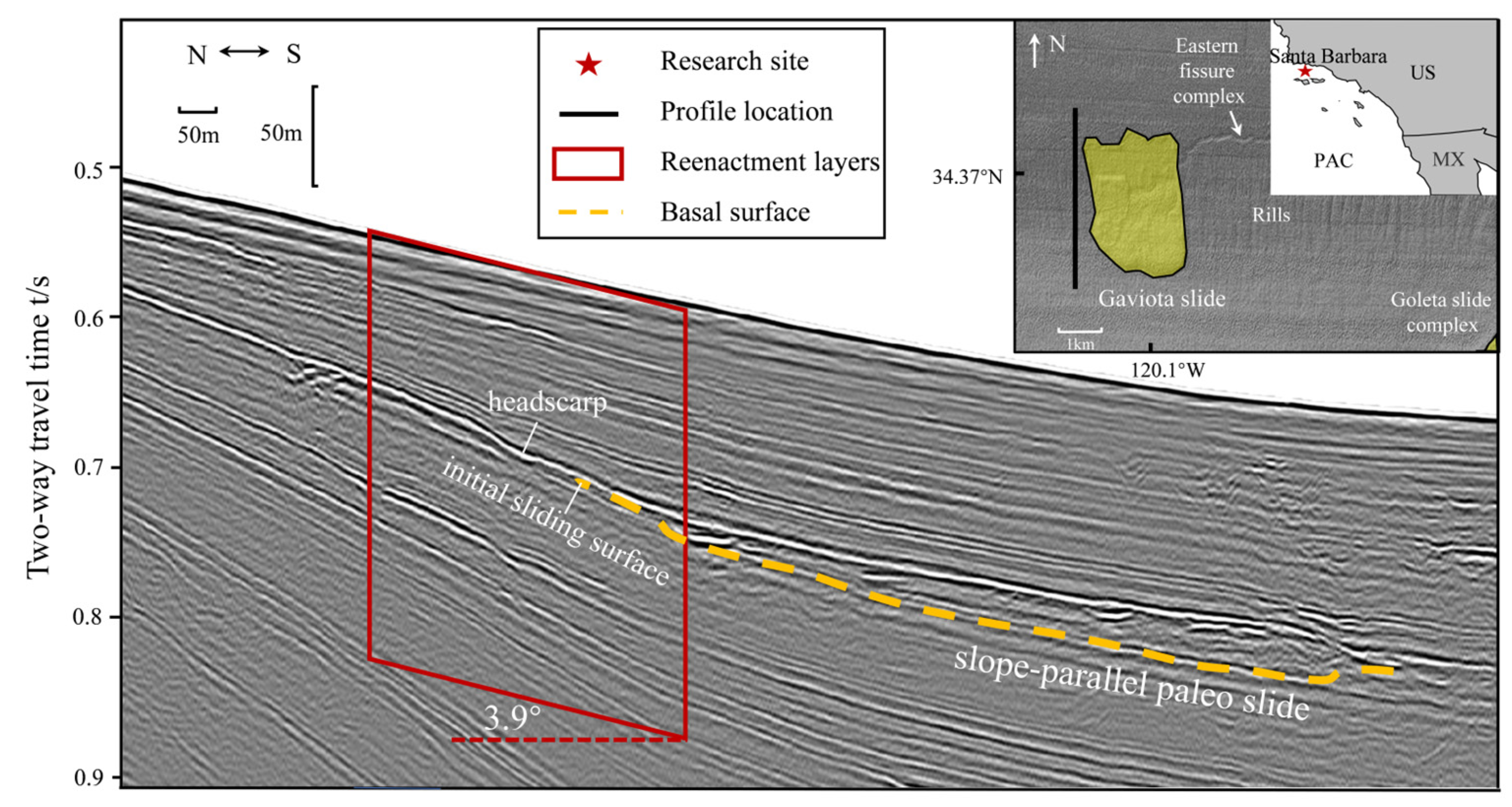
2. Study Area

A case study for sedimentation-stability analysis was conducted in the Santa Barbara basin in the California borderland region. Recent studies [49,50,51,52,53,54,55,56] delineate that the region’s complex geology is marked by steep topographic gradients, unstable sediment layers, and active tectonic features, elevating the risk of submarine landslides. Bathymetric assessments [49,50] reveal considerable variability in the slope steepness within the basin; notably, the northern flank has an average incline of 2.5°, whereas the southern flank presents a gentler slope of 1.7°. The steepest slopes approach 20 degrees near the San Miguel Passage [51].

Sediment provenance studies [52,53] indicate that, from the Holocene (11.9 ka BP) onwards, 60% to 100% of the basin’s sediments originated from the southern slopes of the Santa Ynez Mountains, with an increased contribution during the Last Glacial Maximum (LGM) period. Glacial transport and meltwater flux have significantly contributed to sediment formation in this area. Sediment core sampling within site 893A [54,55,56] reveals that the sedimentation rates here average between 1 and 5 m/kyr, with silty clay and clayey silt being the predominant sediment types.

Moreover, the basin is situated along the North Channel (NC) fault, leading to frequent seismic activities. Recent seismic investigations [35] have highlighted the basin’s vulnerability to seismic events and the potential for tsunamis. Studies [35,49,53] have revealed numerous historical landslides within the basin, with the Goleta landslide being the most voluminous, containing an estimated volume of 1.51 km³. The Goleta landslide complex spans approximately 14.6 km in length and 10.5 km in width, descending to a depth of around 570 m depth, with an average slope angle of 2° [53]. A distinctive feature of this landslide complex is its composition from a series of episodic slope failures, which do not coincide precisely with the seismic event cycles [47]. This observation underscores the significant pre-conditioning role that rapid sedimentation plays in submarine landslide initiation [47]. The landslides within this complex are identifiable on seismic reflection data by their low reflectivity and irregular surface topography, indicating substantial mass wasting events. These landslides have been primarily active during the Holocene, with notable activity around 8 ka and 10 ka [53]. The landslide material predominantly comprises late Pleistocene and Holocene sediments, initially rapidly sedimented in a shelf-edge delta before sliding [50]. The Gaviota landslide, situated west of the Goleta complex, is another notable historical landslide. This landslide involves shallow slope sediment and has been primarily characterized by retrogressive slumping and a fissure extending from the head scarp. It covers an area of 3.78 km² under a water depth of 400–500 m. The failure of this landslide starts on a slope of 4° and ends at 1° [53]. Seismic data [35] suggest that the Gaviota landslide is relatively young, likely a few hundred years old, and affects only the uppermost sediment layers. This landslide’s material moved northeastward and was triggered by similar mechanisms—rapid sedimentation, seismic excitation, oversteepening from structural deformation, and potential fluid mobilization [50,53].

Considering the strong correlation between the triggering of the landslide and rapid sedimentation, a sedimentary reenactment of a typical sloping seabed in the Santa Barbara basin is performed to capture the accumulation of excess pore pressure, the appearance of weak layers, and the subsequent decrease in slope stability throughout the sedimentation process. The case is based on the Multichannel Minisparker seismic-reflection survey conducted by the United States Geological Survey in 2016 [57], as depicted in Figure 1. The seismic reflection profile provides evidence of a historical mass transport event, with the headwall of the slide situated at a water depth of 380 m and the toe deposit at a depth of 406 m. The slide measures approximately 1.1 km in length, and failure initiation occurs in the upper part of the sediment deposits, on a slope with an estimated inclination of 3.9°, based on the initial sliding surface. Despite the significant downslope erosive effects during the extensive deformation and translational phase of the landslide, it can still be conceptualized as a slope-parallel landslide during the subsequent minor deformation stage post-triggering, and the sliding surface is assumed to be a planar surface parallel to the slope.

3. Methodology

Notation: Boldface donates tensors. Dots (˙) denote time derivatives. The prime symbol (′) indicates effective values for stress.

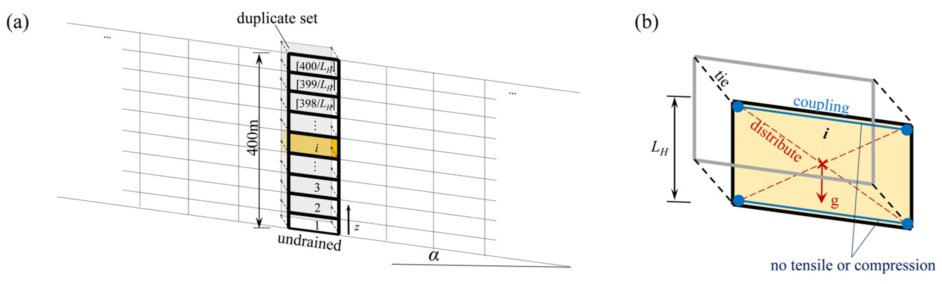
3.1. Governing Equations in the Sedimentation Process

During the sedimentation process, under the influence of gravity, the sedimentary layers gradually compress and consolidate, leading to an increase in the density of the sediment layers and a decrease in porosity, thereby enhancing the strength and permeability of the sediments. However, impeded drainage also leads to the accumulation of excess pore water pressure, which reduces the effective stress within the sediments and consequently diminishes their strength. To simulate the consolidation–seepage process in the saturated porous medium during sedimentation, a commonly used u-p-formulation is used, where the principal variables are the pore pressure, p_w, and displacement of the solid phase, u_s. The continuity equation is applied [58,59]:

$$\nabla \cdot \mathit{v}+{\dot{\epsilon }}_v+\frac{{\dot{p}}_w}{Q}=0$$

(1)

where v is the relative velocity between water and soil, ${\dot{\epsilon }}_v$ is the change in the volumetric strain of the soil skeleton, ${\dot{p}}_w$ is the change in pore pressure (compression corresponds to p_w > 0), and Q is the bulk modulus of the soil–water mixture. Assuming the fluid flow is modeled by Darcy’s law, the relative velocity between water and soil, v, can be calculated as follows [60,61]:

$$\mathit{v}=\frac{k}{{\gamma }_w}\left(-\nabla (\Delta p_w)\right)$$

(2)

where k is the hydraulic conductivity, γ_w is the specific weight of water, and Δp_w is the excess pore pressure. The change in the volumetric strain of soil skeleton, ${\dot{\epsilon }}_v$, in Equation (1) is given by the following:

$${\dot{\epsilon }}_v=\mathit{I}\cdot \frac{\partial {\epsilon }_{\mathit{s}}}{\partial t}$$

(3)

where I is the second-order unit tensor. The soil skeleton strain tensor is ${\epsilon }_{\mathit{s}}=\nabla {\mathit{u}}_{\mathit{s}}$, where u_s is the displacement of the solid phase. According to Terzaghi’s [62] effective stress principle, the total stress, σ, is linked to the fluid pore pressure by the following:

$$\mathit{\sigma } \prime =\mathit{\sigma }-p_w\mathit{I}$$

(4)

where $\sigma \prime$ is the effective stress tensor, satisfying the constitutive relationship with ε_s. The total stress, σ, satisfies the equilibrium equation for mechanical deformation. To simulate the seepage and consolidation process in the sediment layer, a coupled hydro-mechanical finite element (FE) approach is employed within the ABAQUS computing environment [63] The CPE4P element type is employed to replicate the sedimentary processes.

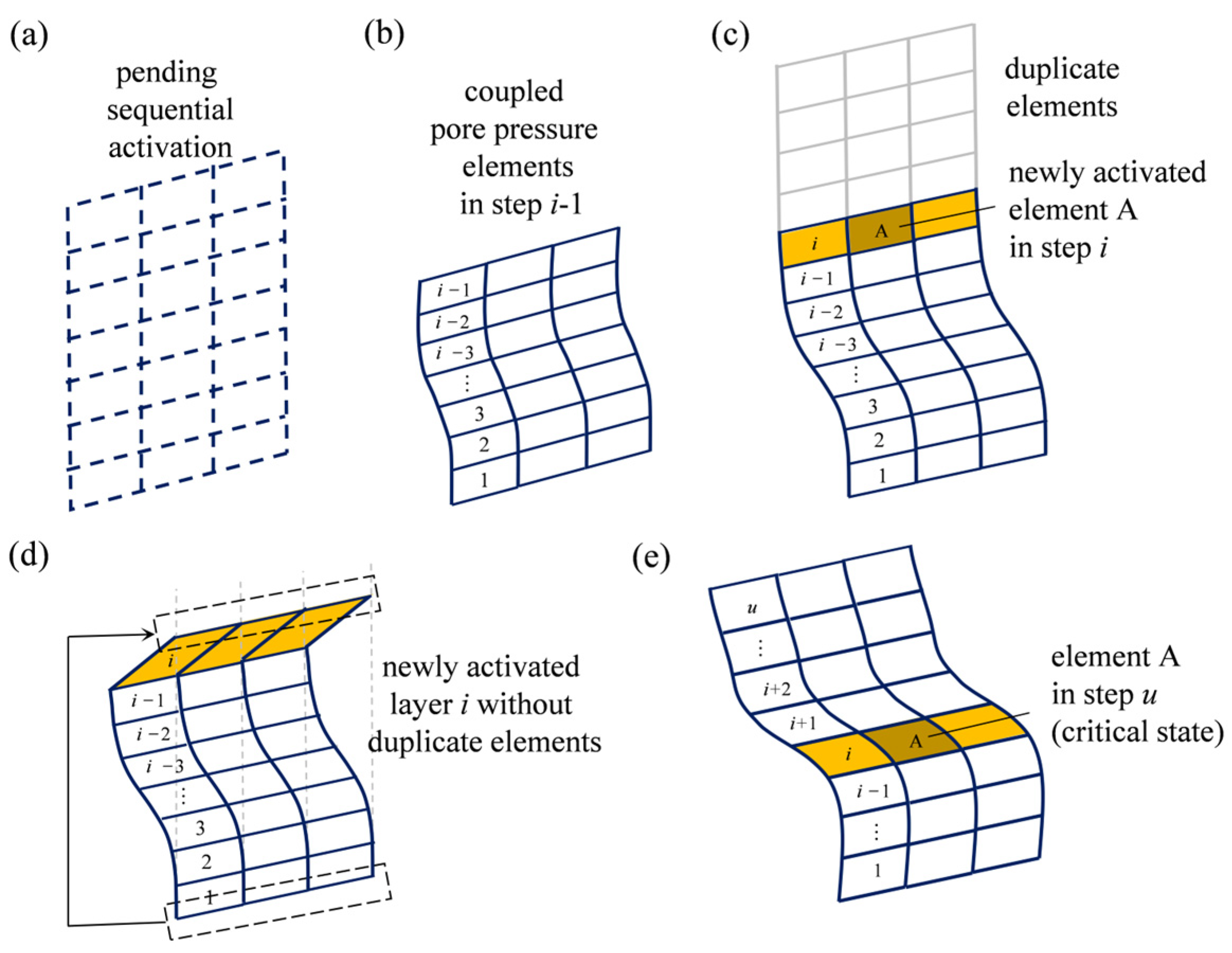
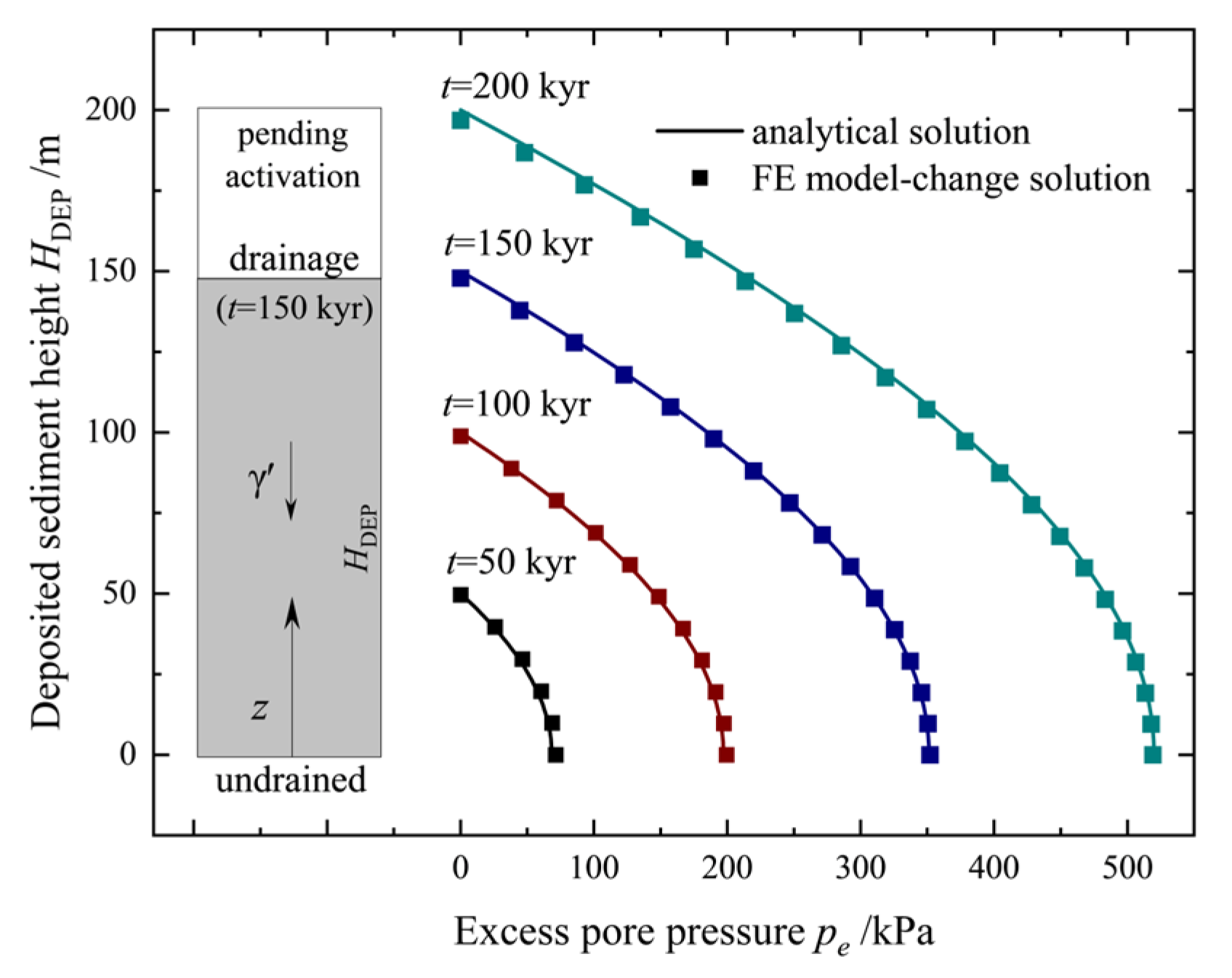
3.2. Implementation, Validation, and Calibration of the Sedimentation Process

To address the challenge of dynamically adapting the geometry model during sedimentation, the FE model-change approach is utilized. The sedimentological problem can be simplified as a gradual formation of a sediment layer on a sloping base. The specific implementation process is shown in Figure 2. The initial state comprises a series of sedimentary layers pending sequential activation (Figure 2a). In the incremental sedimentation process (e.g., from Step i − 1 to Step i), a layer of coupled pore pressure elements is activated and added on top of the existing elements in each new step, with their consolidation time determined by the sedimentation rate (from Figure 2b to Figure 2c). To account for settlement and plastic deformation during sedimentation, which can change the positions of the newly activated layers, a duplicate set of elements is introduced (Figure 2c). These duplicate elements have the same original locations as the activated layers but do not possess pore pressure degrees of freedom (CPE4). They are assigned very low stiffness and serve solely as persistent background grid duplicates. The duplicate elements help track the correct position of the pending activation elements by tying their nodes with the pore pressure elements, and the comparison without a duplicate set is shown in Figure 2d. With further sedimentation, the sediment gradually develops weak layers due to inadequate drainage, wherein certain elements, under increasing shear stress, eventually reach a critical state at step u (Figure 2e). This marks the culmination of the complete process of sedimentation-induced instability of a sloping seabed. The pre-processing for the aforementioned numerical simulation is conducted using ABAQUS scripts.

To validate the FE model-change approach for modeling slopes under rapid sedimentation, a one-dimensional deposited soil column benchmark developed by Gibson [39] is simulated. The benchmark involves a linear elastic soil column subjected to uniform sedimentation along the direction of gravity on a flat impermeable base. The sedimentation rate, r; compression modulus, E_s; hydraulic conductivity, k; and effective bulk density of the soil, γ′, remain constant during the sedimentation process. The analytical solutions for the distribution of pore pressure are as follows [39]:

$$p_e(z,t)={\gamma }^{\prime }rt-{\gamma }^{\prime }{(\pi c_{v}t)}^{-0.5}\exp \left(-\frac{z^2}{4c_{v}t}\right)\cdot {\displaystyle {\int }_0^{\infty }\xi }\tanh \frac{r\xi }{2c_v}\cosh \frac{z\xi }{2c_{v}t}\exp \left(\frac{-{\xi }^2}{4c_{v}t}\right)d\xi$$

(5)

where p_e is the excess pore pressure; z is the vertical distance of the unit from the base; t is the time; γ′ is the effective bulk density; r is the sedimentation rate; and $c_v=k\cdot E_s/{\gamma }_w$ is the coefficient of consolidation, where γ_w = 10 kN/m³ is the bulk density of water.

For the numerical simulation, a one-dimensional soil column with a total heigh of $H_{\mathrm{ACT}}^S$ = 200 m is used, divided into a layer height of L_H = 10 m each, to simulate the sedimentation process. In the analysis, the sediment is assumed to be linearly elastic, with a compression modulus of E_s = 10 kPa. Duplicate grid copies with very low stiffness are employed, featuring a bulk modulus of E′ = 0.1 Pa. No creep or viscoelastic behavior is considered. Drainage boundary conditions are applied on the upper surface of the newly active sediment layers, while the nodes at the lateral boundaries are constrained from horizontal movement, and the nodes at the bottom are fixed. The parameters used for comparison are listed in

Table 1. Hydraulic coupling parameters of the replicated elastic sediments used for validation.

Parameter	Value (Unit)
Sedimentation rate, r	1.0 m/kyr
Compression modulus of the sediment, Es	10 MPa
Poisson’s ratio, υ	0
Bulk modulus of duplicate grid copies, E′	10 Pa
Hydraulic conductivity of the sediment, k	0.05 m/kyr
Effective bulk density of the sediment, γ′	5 kN/m3
Bulk density of water, γw	10 kN/m3
Layer height, LH	10 m
$\mathrm{Total} \mathrm{height} \mathrm{of} \mathrm{the} \mathrm{column}, H_{\mathrm{ACT}}^S$	200 m

. The hydraulic conductivity of the sediment is k = 0.05 m/kyr, and the effective bulk density is γ′ = 5 kN/m³. The sedimentation rate is regarded as r = 1.0 m/kyr. The comparison of pore pressure, p_e, between the analytical solution and the numerical solution at various sedimentation times, t, reveals a robust agreement (Figure 3). These findings affirm the precision of the finite element (FE) model-change approach in computing the cumulative pore pressure throughout the sedimentation process. The observed discrepancies are attributed to an artificially extended drainage path resulting from the discretization of activated layers. It is evident that reducing the layer thickness can help mitigate these discrepancies. Therefore, early calibration of layer thickness parameters is deemed necessary in the proposed FE model-change approach.

Herein, to address the potential underestimation of excess pore pressure resulting from sparse artificial layer partitioning, a calibration procedure for layer thickness, L_H, which is equivalent to mesh size, is implemented within the FE model-change approach. Moreover, to ensure the generalizability of the conclusions, the layer height parameter, L_H, is normalized, and the activated number of layers, N_L, is introduced:

$$N_L=⌈H_{\mathrm{ACT}}^S/L_H⌉$$

(6)

where N_L is the activated layer number when the failure occurs, and $H_{\mathrm{ACT}}^S$ is the height of the activated sediment when the failure occurs. The calibration process selects the maximum excess pore pressure, p_e,max, and minimum void ratio, e_min, in the sediment as evaluation parameters. These parameters provide a comprehensive assessment of the variations in the seepage and stress field, which directly influence slope stability. As the calibration parameters gradually stabilize within a certain error range, it is considered that the mesh size (i.e., the L_H) at this point is sufficiently small.

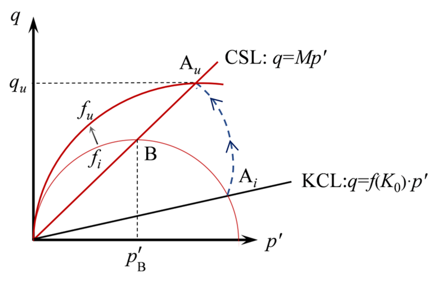
3.3. The Modified Cam-Clay (MCC) Model

During the sedimentation process of the slope, to simulate the consolidation behavior of sediments, the well-established Modified Cam-Clay (MCC) model [64] was used for the representation of the constitutive behavior. It captures a strong increase in stiffness with advancing compaction and contractive behavior during the shearing of the sediments. The yield surface, f, for the MCC model is given by the following [64]:

$${(p^{\prime }-{p^{\prime }}_B)}^2+{(\frac{q}{M})}^2={({p^{\prime }}_B)}^2$$

(7)

where p′ is the mean equivalent stress; ${p^{\prime }}_B$ is a strain hardening parameter corresponding to a plastic component of volumetric strain, ${\epsilon }_v^p$; q is the deviatoric stress; and M is the inclination of the critical state line. The yield function f > 0 defines admissible stress states in an elastoplastic continuum (Figure 4). When the plastic deformation is compressive (${\epsilon }_v^p>0$), ${p^{\prime }}_B$ will increase, causing the yield surface, f, to grow in size. A typical sedimentation process of soil element A is shown (from Figure 2c to Figure 2e), which forms an undrained path (Figure 4) from its initial state on the K₀ consolidation line (A_i) to the CSL line (A_u). During the process, the yield surface hardens (f_i→f_u) due to the increased ${\epsilon }_v^p$, and A_u is located at the highest point of the yield function, f_u. The peak deviatoric stress, q_u, of A_u is given by the following [47]:

$$q_u=M{p}^{\prime }{\left(\frac{1}{2}+\frac{q^2}{2M^2{p^{\prime }}^2}\right)}^{\Lambda }, \Lambda =1-\frac{\kappa }{\lambda }$$

(8)

where Λ is the normalized parameter and represents the relative length between $\stackrel{⏜}{A_{i}B}$ and $\stackrel{⏜}{A_i{A}_u}$, κ is the log bulk modulus, and λ is the log plastic bulk modulus.

3.4. Stability Analysis Methods for Sedimenting Slopes

In order to quantify the real-time stability of slopes during rapid sedimentation processes, it is imperative to elucidate a computational method. By considering the static equilibrium of sediment layers at each instant, the following equations can be derived [64,65]:

$$F_S^A=\min \left\{\frac{{\displaystyle \sum _{j=1}^{n_j}{q}_u^j}}{{\displaystyle \sum _{j=1}^{n_j}{q}^j}}\right\}$$

(9)

$$F_S^B=\min \left\{\frac{{\displaystyle \sum _{j=1}^{n_j}{s}_u^j}}{{\displaystyle \sum _{j=1}^{n_j}{\tau }_g^j}}\right\}$$

(10)

where $F_S^A$ is the safety factor based on the stress state of the soil element; j represents the jth possible failure path (out of a total of n_j paths); $F_S^B$ is the safety factor based on the ratio of resisting shear force to driving shear force; s_u the undrained shear strength; and τ_g is the gravitational shear stress, which is obtained by integrating the effective density, ρ′, over the height of the current sediment, given by the following:

$${\tau }_g(z)=g\sin \alpha \cdot {\displaystyle {\int }_z^{H_{\mathrm{DEP}}}\frac{{\rho }_s+{\rho }_w\cdot e(z)}{1+e(z)}-{\rho }_w\mathrm{d}z}$$

(11)

where z is the vertical distance of the current element from the corner of the slope; g is the gravitational acceleration, 10 m/s²; α is the slope angle; H_DEP is the varying height of the deposited sediment; ρ_s is the soil grain density; ρ_w is the water density, 1 g/cm³; and e is the void ratio.

In addition, the undrained shear strength, s_u, in Equation (10) is multiplicatively related to the peak deviatoric stress, q_u, given by the following:

$$s_u=\left\{\begin{array}{c}\frac{q_u}{2}\mathrm{if} \dim =3\\ \frac{q_u}{\sqrt{3}} \mathrm{if} \dim =2\end{array}\right.$$

(12)

where dim is the question dimension, and dim = 2 (for plane strain analysis) or 3. It is evident that the safety factor, $F_S^A$, is more accurate and conservative compared to the effective stress ratio, Mp′/q (i.e., projection of A_i on the CSL) (Figure 4), while $F_S^B$ reflects the essence of slope shear failure. The specific stability assessment metric to be employed is elaborated upon in the following sections.

4. Sedimentary Recurrence and Stability Analysis

4.1. Modelling and Parameterization

Herein, a two-dimensional plane strain infinite slope model is utilized to replicate the sedimentation process and to represent the slope-parallel landslide (Figure 5a). This simplification allows for the determination of the sliding surface depth, while reducing computational expenses and eliminating the need for a search along the slope for the sliding surface [66,67]. This simplification is more applicable to areas with gentle slopes, such as continental shelves. Based on sediment cores and geophysical data [68], the overall slope angle is determined to be a = 3.9°, and the average sedimentation rate in the research area is determined to be r = 4.24 m/kyr. The sedimentary phases primarily consist of nearshore and semi-deep-sea phases along continental margins, and the MCC model is utilized to characterize the silty clay or the clayey silt. The density of the soil grains is ρ_s = 2.7 g/cm³. It is important to note that, over the long timescale of the sedimentation process, the sedimentation rate and the mechanical properties of the sediment (including the initial stress state upon activation of the MCC model) remain constant [33,47]. Considering the changes in sediment permeability during the process of mechanical compaction, the variation in void ratio, e, and the hydraulic conductivity, k, can be expressed using a commonly used logarithmic relationship [69], with an initial hydraulic conductivity of k₀ = 2 × 10⁻⁹ m/s and an initial void ratio of e₀ = 3.8. The critical state effective stress ratio, M; log plastic bulk modulus, λ; and log bulk modulus, κ, of the sediment are calculated by the following:

$$M=\sqrt{3}\sin {\phi }^{\prime }$$

(13)

$$\lambda =\frac{c_c}{\ln 10}$$

(14)

$$\kappa =\frac{c_s}{\ln 10}$$

(15)

where φ′ is the internal friction angle, c_c is the compression index, and c_s is the swell index. The elements are activated with an initial stress corresponding to the initial density, ρ′, applied at the depth, h₀, below the seafloor. The coefficient of static lateral pressure, denoted as K₀, is defined by the following equation:

$$K_0=0.64+0.001I_P$$

(16)

where I_P is the plastic index. Sediment parameters (shown in Table 1) are extracted from sediment cores collected at site 893 within the Santa Barbara basin [70,71].

To account for the influence of element deformation on the gravity load, a concentrated load equal to the gravity is applied at the centroid of the current layer and then distributed to the nodes of the layer using the continuum coupling approach [33,47]. For the boundary conditions of the plane strain infinite slope, the strain rate, dε_s/dt, along and normal to the slope direction is 0. This is achieved by constraining the rotational degrees of freedom of all nodes and tying the translational degrees of freedom of the nodes on one side of the sediment column to the corresponding nodes on the other side (Figure 5b). A dynamically varying hydraulic boundary is consistently applied to the top of the sediments. In addition, a duplicate set of elements with a bulk modulus of E′ = 0.1 Pa are employed. To capture potential sliding surfaces, the initial total height of sediment is set at 400 m. The initial stress, void ratio (e), and hydraulic conductivity (k) are assumed to be uniform within each layer.

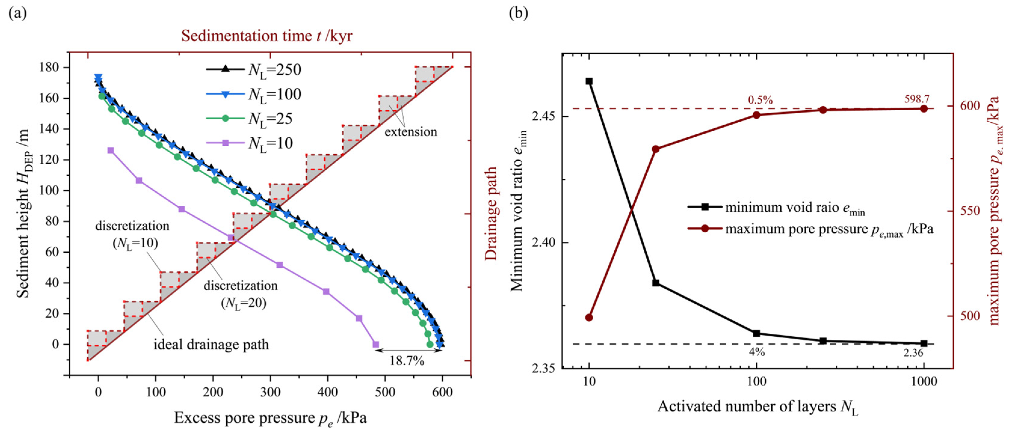
4.2. Calibration of the Layer Height L_H

Based on the calibration method proposed in Section 3.2, numerical simulations were conducted for sedimentation-instability processes under varying parameter conditions, with sediment layer numbers N_L = 10, 25, 100, and 250. The distributions of excess pore pressure, p_e (Figure 6a), and the minimum void ratio, e_min (Figure 6b), obtained from these simulations are utilized for calibration. It is worth noting that, due to the possibility of computational termination during the sedimentation process (attributable to excess element distortion), the activated sediment layer height at the moment of failure, $H_{\mathrm{ACT}}^S$, is employed in Equation (6) instead of the total sediment layer height, H. The observed trend suggests that the utilization of the proposed discretization approach leads to a decrease in excess pore pressure results due to an artificial extension of the drainage path. When N_L > 100, the discrepancies are all below 5%. The trial calculations establish $H_{\mathrm{ACT}}^S$ = 237 m, and the layer thickness is chosen to be L_H = 1 m for subsequent numerical computations.

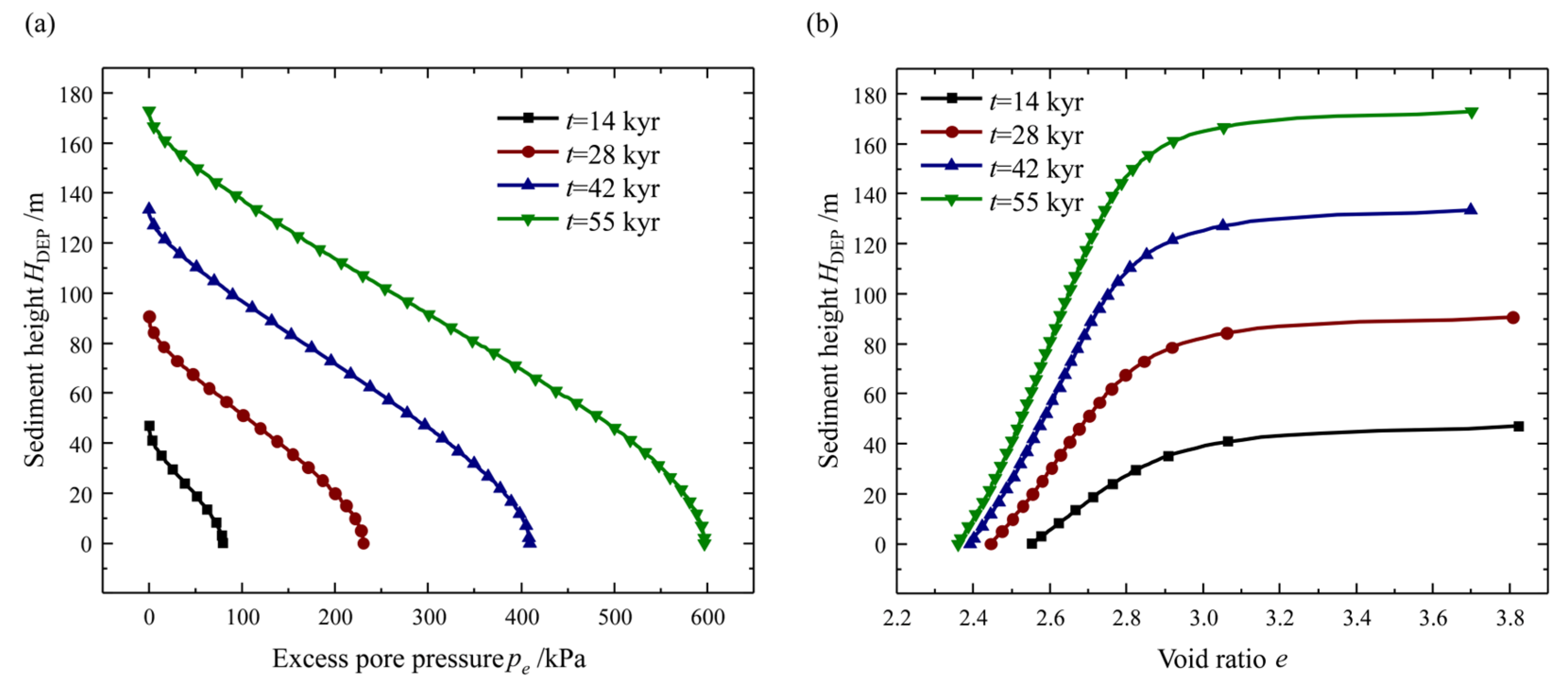
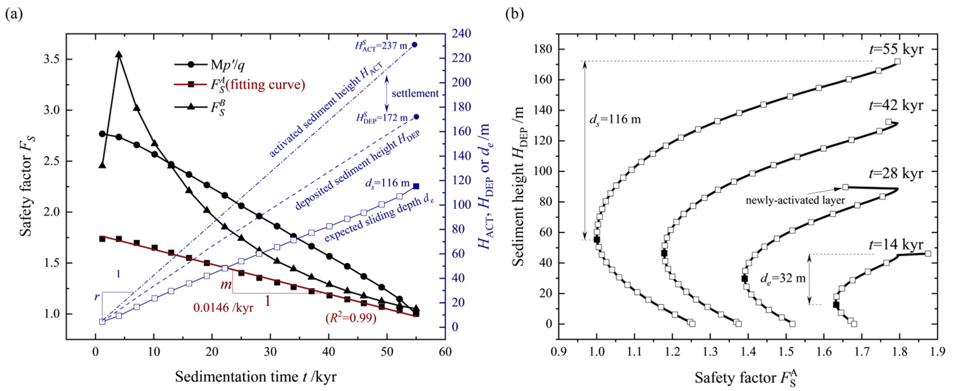
4.3. Result and Analysis

From the temporal distribution of excess pore pressure, p_e, and void ratio, e, during the sedimentation process, it is evident that, except for the surface sediments, the sediment experiences rapid compaction, leading to an accumulation of pore pressure (Figure 7a) and a substantial decrease in the void ratio, e (Figure 7b). As compaction progresses, the permeability of the sediments decreases, thereby increasing the drainage path of the pore fluid and resulting in a greater accumulation of excess pore pressure within the sediment. The accumulated excess pore pressure, p_e, partially counteracts the total stress, consequently decreasing the effective stress and significantly increasing the likelihood of slope failure.

From the results of the slope stability analysis, we can see that all three indicators representing the stability of slopes ($F_S^A$, $F_S^B$, and $M{p}^{\prime }/q$) generally show a downward trend during sedimentation (Figure 8a). This phenomenon can be attributed to the reduction in actual effective stress within the geological strata compared to the current effective sediment load during sedimentation (Figure 7a). Furthermore, the under-consolidated state of the sediment contributes to the weakening of the submarine slope’s stability. Conversely, in the early stage of sedimentation, there is a temporary increase in both effective stress and strength due to relatively higher permeability. This leads to a temporary rise in $F_S^B$ before it subsequently declines. Additionally, the rate of decrease in the safety factor, m, remains consistent over time (R² = 0.99), allowing it to be used for evaluating slope stability during future sedimentation processes (Figure 8a). In conclusion, considering that $F_S^A$ reflects a more conservative and reliable estimate of stability and is simpler to use in predicting stability, $F_S^A$ was selected as the criterion for assessing the stability of rapidly sedimenting slopes (Figure 8a). Based on the temporal distribution of $F_S^A$, the precise depth, d_e, of the expected slide is indicated, and d_e is substituted by d_s (the actual depth of the sliding surface) when a failure occurs ($F_S^A$ < 1) (Figure 8b). The results demonstrate that the d_e undergoes a linear descent throughout the sedimentation process. These findings provide valuable insights into predicting the expected depth of landslides that may occur during future sedimentation processes.

Herein, the spatial variation in the undrained shear strength, s_u, within the sediment throughout the sedimentation process is analyzed (Figure 9). As the sedimentation progresses, the distribution of strength transitions from a linear pattern (t = 14 kyr) to a weakened state in the lower layers (t = 55 kyr) (Figure 9a). This implies that the sedimentation process leads to the formation of a weak layer (compared to a linear increase) within the sediment, which can significantly contribute to slope instability. This is evident from the close match between the depth of the weak layer, d_w, and the expected depth of failure, d_e. Furthermore, the variation in the increasing rate, n, of s_u in the z-direction is depicted and analyzed (Figure 9b). During the early stages of sedimentation (Stage I, 0–4 kyr), the strength of submarine sediments increases, which is consistent with the $F_S^B$ results (Figure 8a). Moreover, the slope failure can be further divided into three stages based on a safety factor of F_S = 1.5 [72].

5. Parametric Analysis on the Stability of Rapidly Sedimenting Slopes

In order to account for the uncertainty in sedimentation rate parameters, a comprehensive parametric analysis was conducted specifically for sedimentation rates. Furthermore, considering the long timescale of the sedimentation process, it is more likely that slope instability is triggered by short-term events such as earthquakes rather than solely by sedimentation [73,74]. Therefore, it was crucial to perform stability analyses on rapidly sedimenting submarine slopes under the influence of earthquakes. In our study, a parametric analysis of the loading pattern of seismic events and the timing of seismic events was undertaken.

5.1. Sedimentation Rate, r

Based on a variable parameter analysis for sedimentation rates, it is observed that there was no failure for a sedimentation rate of r = 1 m/kyr within the given $H_{\mathrm{ACT}}^S$ (approximately 100 kyr), as indicated by $F_S^A$ > 1 (Figure 10a). However, the time to failure can still be predicted using the proposed reduction rate, m. In addition, without considering variations in sediment type and over long timescales, an increase in sedimentation rate leads to a decrease in slope stability, a reduction in the depth of the sliding surface, and a diminution in sediment strength (Figure 10a–c). Based on extensive simulation results covering a range of sedimentation rates from 0.1 m/kyr to 10 m/kyr, an exponential relationship is observed between the sedimentation rate and both the expected sliding surface depth, d_e, and the sediment strength, m. A distinct impact pattern is identified when the slope is stable, indicating a stable slope condition (Figure 10d). These conclusions allow for the determination of the critical sedimentation rate, r_crit (1.33~1.82 m/kyr), that corresponds to slope stability for a specific period of approximately 100 kyr in this case. The findings also enable the simultaneous prediction of the sliding surface depth and the rate of increase in sediment strength, n, for a given sedimentation rate.

5.2. Loading Pattern of Seismic Events

To account for seismic effects, a horizontal acceleration impulse, a_h, is applied. This simplified earthquake loading representation was commonly used in previous studies [74,75,76]. This approach allows for the quantification of variations in excess pore pressure during seismic events and changes in the slope’s safety factor. Specifically, an earthquake loading step is introduced at 14 kyr after sedimentation, where the slope is subjected to a horizontal acceleration impulse of a_h = 0.1 g for a duration of 10 s (Figure 11a). It is important to note that the specific duration of the seismic activity has no influence on the results in comparison to the prolonged temporal scale of pore pressure dissipation. To account for the uncertainty in the direction of vertical loads during earthquakes, various vertical acceleration patterns (Cases A–C) are considered (Figure 11b). For the seismic analysis, the gravitational shear stress,${{\tau }^{\prime }}_g$, is updated to incorporate the seismic loading. The updated seismic shear stress can be calculated based on the following relationship:

$${{\tau }^{\prime }}_g(z)=((1+a_v)\sin \alpha +a_h\cos \alpha )\mathrm{g}\cdot {\displaystyle {\int }_z^{H_{\mathrm{DEP}}}\frac{{\rho }_s+{\rho }_w\cdot e(z)}{1+e(z)}-{\rho }_w\mathrm{d}z}$$

(17)

where a_v is the current vertical seismic acceleration, and a_h is the current horizontal seismic acceleration. The parameters of the MCC model for the sediments are consistent with those listed in

Table 2. Parameters of the sediments based on the Modified Cam-Clay model used for the replication of the sedimentary layer [70,71].

Parameter	Value (Unit)
Slope inclination, α	3.9°
Initial void ratio, e0	3.8
Internal friction angle, φ′	30°
Initial hydraulic conductivity, k0	2 × 10−9 m/s
Compression index, cc	0.6
Swell index, cs	0.15
Average sedimentation rate, r	4.24 m/kyr
Density of the soil grains, ρs	2.7 g/cm3
Initial stress-required height, h0	0.3 m
Plastic index, IP	35
Hydraulic conductivity, k	$k=2\times {10}^{\frac{e-3.6}{0.4}-9}\mathrm{m}/\mathrm{s}$

. The stability of slopes under three distinct loading patterns is presented (Figure 11d,e).

It is observed that when the vertical acceleration of the seismic loadings aligns with the direction of gravity (Case B), there is a more significant increase in excess pore pressure (Figure 11c), causing a more severe decrease in sediment strength and an accelerated destabilization process. The findings indicate that, compared to the compaction effects that result in looser sediment (upward vertical acceleration, Case C), the impact of downward acceleration, a_v, on the increase in downslope force (downward vertical acceleration, Case B) is more pronounced, making it the most unfavorable condition among the various seismic load combinations (Figure 11c,d). As $F_S^A$ effectively captures differences between various loading patterns and provides more conservative results, it is considered an indicator for evaluating the seismic stability of rapidly sedimenting submarine slopes. In all three cases, the slope safety factor, $F_S^A$, rapidly decreases to 1.0 within 10 s, with a rate of decrease in the safety factor during the seismic event, m_seismic = 0.143/s (Figure 11d). The obtained acceleration combination (Case B) is considered the most critical condition and will be applied in further analyses considering different seismic trigger times.

Additionally, to evaluate the individual contributions of seismic events and pre-processing factors to slope instability, a relative rate of decrease in the safety factor m* is established:

$$m*=\frac{m_{\mathrm{seismic}}}{m}$$

(18)

A larger value of m* indicates a greater contribution of the seismic activity in triggering instability. The evaluation of the relative rate of decrease in the safety factor provides insights into the contributions of seismic events and pre-conditioning factors in triggering slope instability.

5.3. Occurrence Timing of Seismic Events, t*

To accurately assess the stability of rapidly sedimenting submarine slopes under earthquakes with different trigger moments, it is important to consider the timing of seismic events. In this study, a dimensionless parameter, t*, is used to quantify the ratio of the earthquake moment to the overall duration of slope sedimentation. Building upon the previously obtained most critical load combination, the effects of different trigger times for seismic events (Cases B, D, and E) on slope stability are analyzed and presented (Figure 12a,e). The analysis reveals that, as the occurrence time of seismic events is delayed, weak layers gradually form within the slope, leading to a decrease in slope stability. This is reflected in the reduced seismic resistance of the slope (Figure 12b–d). Moreover, it is noted that earthquakes interrupt the downward movement of the sliding surface during sedimentation (Figure 12e), leading to shallower sliding surfaces in comparison to slopes unaffected by seismic activity. During an earthquake event, the sliding surface undergoes no significant changes within a short duration. As a result, the post-earthquake sliding surface depth remains consistent with the expected sliding surface depth obtained through the static sedimentary analysis (Figure 12f–h). The observations presented in this study aid in the prediction of the depth of the sliding surface following an earthquake. Additionally, the critical horizontal acceleration, which represents the minimum acceleration required to induce slope failure, gradually decreases with the increasing time delay and exhibits an approximately linear correlation with the occurrence time, t* (Figure 12i). The critical horizontal acceleration values obtained in this study are in good agreement with those reported by Lee et al. [77], further validating the reliability of the proposed approach. These findings provide valuable insights for predicting the potential instability of a slope under specific seismic activity levels and also have significant implications for identifying past seismic fault events in the area.

6. Conclusions

The study proposes a methodology that combines the calibrated FE model-change approach with a real-time stability analysis method to effectively assess and predict the stability of submarine slopes under rapid sedimentation processes. The following conclusions are drawn:

• To evaluate the reliability of the FE model-change approach, a crucial dimensionless number, N_L, is proposed as a calibration metric, and the method is deemed accurate when N_L > 100. The calibrated numerical approach effectively replicates the sedimenting process of submarine slopes and accurately captures the accumulation of excess pore pressure, the reduction in strength, and the instability of the submarine slope.
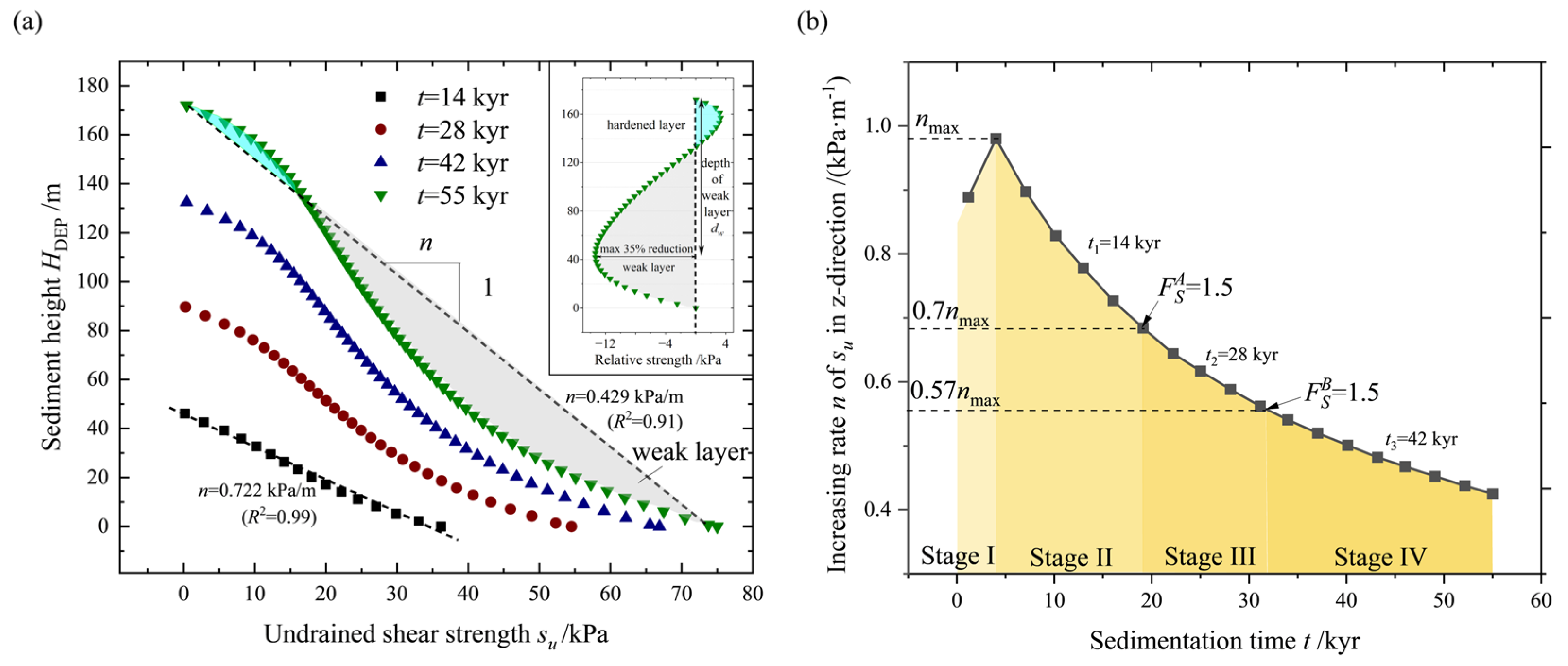
• $F_S^A$ is proposed as a conservative metric for assessing the stability of submarine slopes during rapid sedimentation, and its decreasing rate, m, is introduced to predict the slope stability within a specific period. The distribution of strength transitions from a linear pattern to a weakened state, which is considered a key factor triggering slope instability.
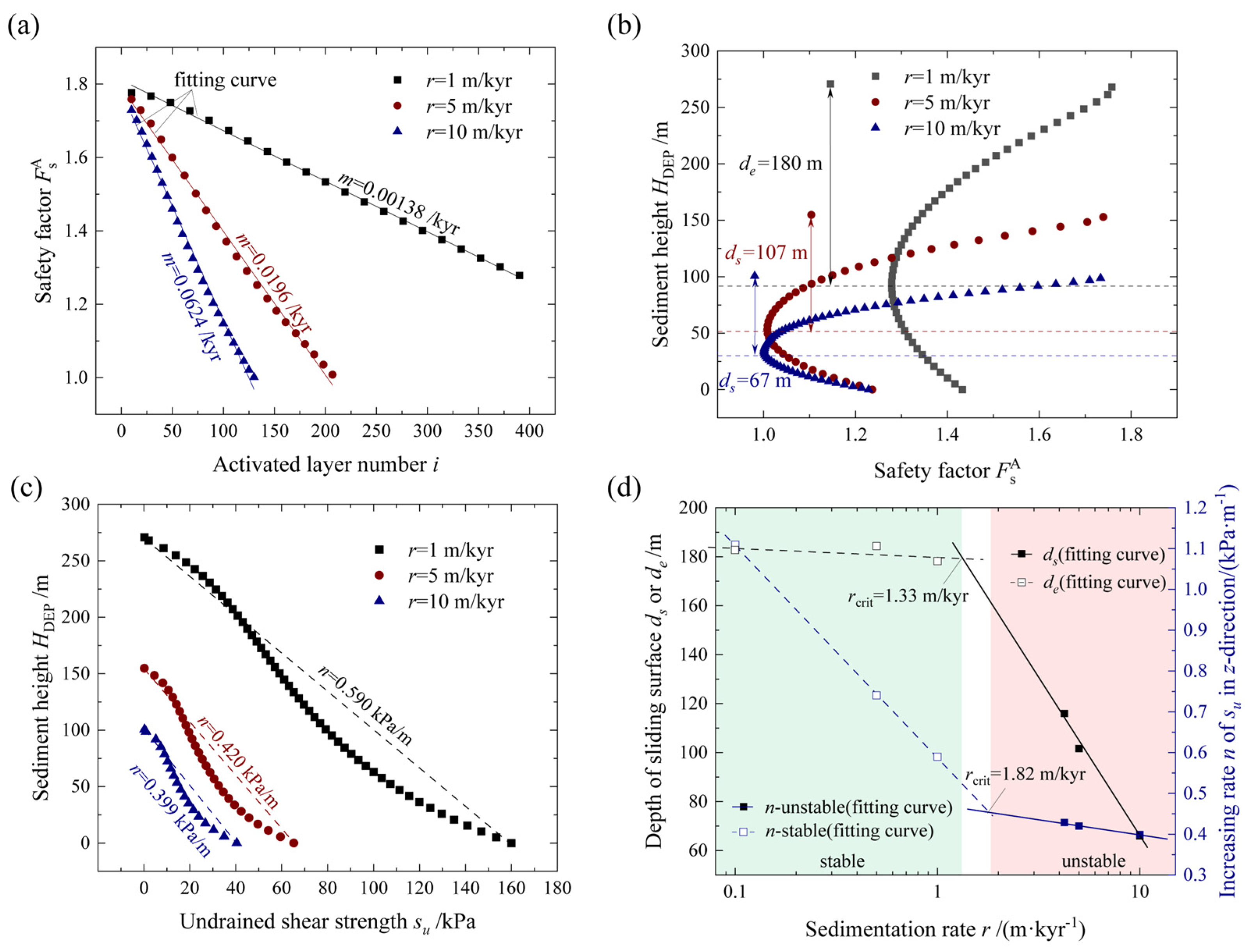
• Through a variable parameter analysis of sedimentation rates, it is concluded that an increase in the sedimentation rate makes shallow landslides more prone to occurrence. A further analysis of the sediment strength and sliding surface depth yields a method for calculating the critical sedimentation rate.
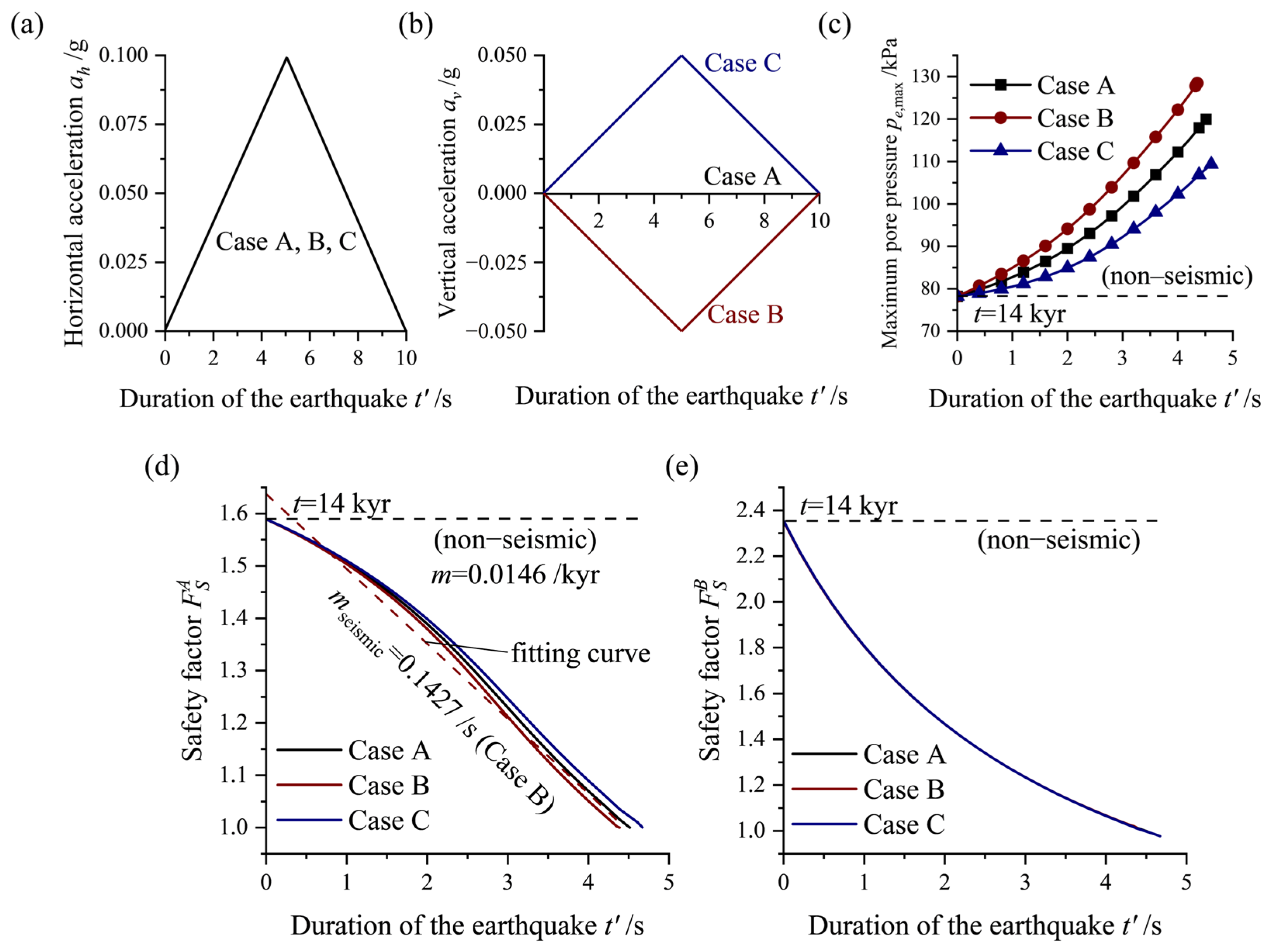
• In assessing the stability of rapidly sedimenting slopes under seismic action, the most critical condition compared to other load combinations is determined. To quantify the individual impacts of seismic events and rapid sedimentation on slope instability, a relative rate of decrease in the safety factor, m*, is proposed.
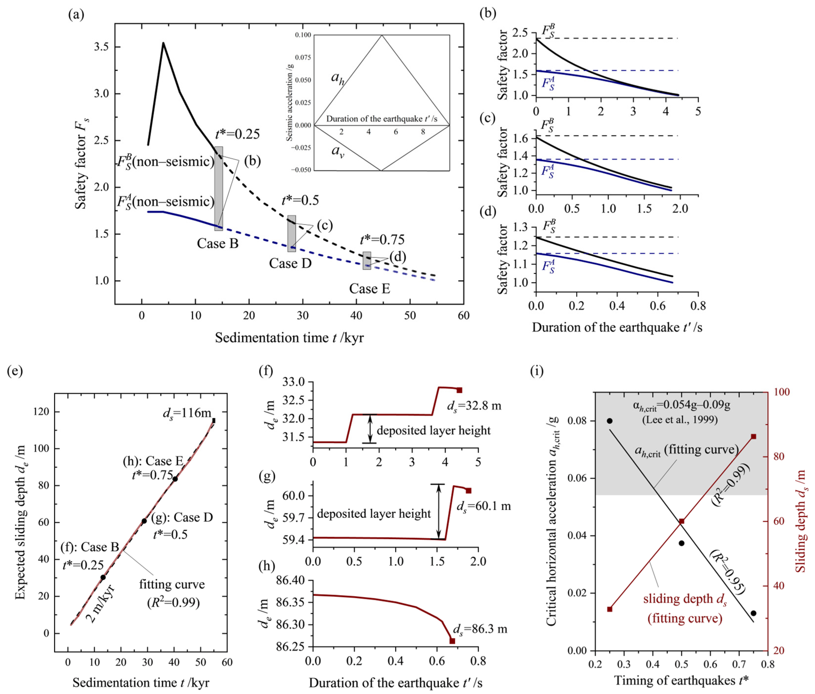
• During the sedimenting process, earthquake events prematurely interrupt the downward movement trend of the sliding surface, leading to a shallower sliding surface. Additionally, a method for calculating the critical horizontal seismic acceleration of the slope is proposed. Furthermore, the relevant results help to identify potential historical seismic fault events.

References

- Guo, X.; Fan, N.; Zheng, D.; Fu, C.; Wu, H.; Zhang, Y.; Song, X.; Nian, T. Predicting impact forces on pipelines from deep-sea fluidized slides: A comprehensive review of key factors. Int. J. Min. Sci. Technol. 2024, 34, 211–225. [Google Scholar] [CrossRef]
- Guo, X.; Liu, X.; Li, M.; Lu, Y. Lateral force on buried pipelines caused by seabed slides using a CFD method with a shear interface weakening model. Ocean Eng. 2023, 280, 114663. [Google Scholar] [CrossRef]
- Talling, P.J.; Clare, M.L.; Urlaub, M.; Pope, E.; Hunt, J.E.; Watt, S.F. Large submarine landslides on continental slopes: Geohazards, methane release, and climate change. Oceanography 2014, 27, 32–45. [Google Scholar] [CrossRef]
- Hampton, M.A.; Lee, H.J.; Locat, J. Submarine landslides. Rev. Geophys. 1996, 34, 33–59. [Google Scholar] [CrossRef]
- Zhu, Z.; Wang, D.; Zhang, W. Catastrophic submarine landslides with non-shallow shear band propagation. Comput. Geotech. 2023, 163, 105751. [Google Scholar] [CrossRef]
- Zhang, W.; Klein, B.; Randolph, M.F.; Puzrin, A.M. Upslope failure mechanisms and criteria in submarine landslides: Shear band propagation, slab failure and retrogression. J. Geophys. Res. Solid Earth 2021, 126, e2021JB022041. [Google Scholar] [CrossRef]
- Puzrin, A.M.; Germanovich, L.N.; Friedli, B. Shear band propagation analysis of submarine slope stability. Géotechnique 2016, 66, 188–201. [Google Scholar] [CrossRef]
- Yenes, M.; Monterrubio, S.; Nespereira, J.; Casas, D. Apparent overconsolidation and its implications for submarine landslides. Eng. Geol. 2020, 264, 105375. [Google Scholar] [CrossRef]
- Kaminski, P.; Sager, T.; Grabe, J.; Urlaub, M. A new methodology to assess the potential of conjectural trigger mechanisms of submarine landslides exemplified by marine gas occurrence on the Balearic Promontory. Eng. Geol. 2021, 295, 106446. [Google Scholar] [CrossRef]
- Nian, T.; Shen, Y.; Zheng, D.; Lei, D. Research advances on the chain disasters of submarine landslides. J. Eng. Geol. 2021, 29, 1657–1675. (In Chinese) [Google Scholar] [CrossRef]
- Guo, X.; Liu, X.; Zheng, T.; Zhang, H.; Lu, Y.; Li, T. A mass transfer-based LES modelling methodology for analyzing the movement of submarine sediment flows with extensive shear behavior. Coast. Eng. 2024, 191, 104531. [Google Scholar] [CrossRef]
- Guo, X.; Fan, N.; Liu, Y.; Liu, X.; Wang, Z.; Xie, X.; Jia, Y. Deep seabed mining: Frontiers in engineering geology and environment. Int. J. Coal Sci. Technol. 2023, 10, 23. [Google Scholar] [CrossRef]
- Zheng, D.F.; Nian, T.K.; Liu, B.; Liu, M.; Yin, P.; Huo, Y.D. Investigation of the stability of submarine sensitive clay slopes under wave-induced pressure. Mar. Georesour. Geotechnol. 2019, 37, 116–127. [Google Scholar] [CrossRef]
- Shan, Z.; Wu, H.; Ni, W.; Sun, M.; Wang, K.; Zhao, L.; Lou, Y.; Liu, A.; Xie, W.; Zheng, X.; et al. Recent technological and methodological advances for the investigation of submarine landslides. J. Mar. Sci. Eng. 2022, 10, 1728. [Google Scholar] [CrossRef]
- Fan, N.; Jiang, J.; Nian, T.; Dong, Y.; Guo, L.; Fu, C.; Tian, Z.; Guo, X. Impact action of submarine slides on pipelines: A review of the state-of-the-art since 2008. Ocean Eng. 2023, 286, 115532. [Google Scholar] [CrossRef]
- Bea, R.G. How sea floor slides affect offshore structures. Oil Gas J. 1971, 69, 88–92. [Google Scholar]
- Sterling, G.H.; Strohbeck, E.E. The Failure of the South Pass 70 “B” Platform Hurricane Camille. In Proceedings of the Offshore Technology Conference, Houston, TX, USA, 28 April 1973. [Google Scholar] [CrossRef]
- Hsu, S.K.; Kuo, J.; Chung-Liang, L.; Ching-Hui, T.; Doo, W.B.; Ku, C.Y.; Sibuet, J.C. Turbidity currents, submarine landslides and the 2006 Pingtung earthquake off SW Taiwan. Terr. Atmos. Ocean. Sci. 2008, 19, 7. [Google Scholar] [CrossRef]
- Nian, T.K.; Gu, Z.; Guo, X.; Zhang, H.; Jia, Y. Effect of temperature rise on the mechanical behaviour of deep-sea clay surrounding oil and gas pipelines. Ocean Eng. 2024, 302, 117533. [Google Scholar] [CrossRef]
- Wang, Z.; Zheng, D.; Guo, X.; Gu, Z.; Shen, Y.; Nian, T. Investigation of offshore landslides impact on bucket foundations using a coupled SPH–FEM method. Geoenviron. Disasters 2024, 11, 2. [Google Scholar] [CrossRef]
- Pszonka, J.; Wendorff, M.; Godlewski, P. Sensitivity of marginal basins in recording global icehouse and regional tectonic controls on sedimentation. Example of the Cergowa Basin, (Oligocene) Outer Carpathians. Sediment. Geol. 2023, 444, 106326. [Google Scholar] [CrossRef]
- Moernaut, J.; De Batist, M. Frontal emplacement and mobility of sublacustrine landslides: Results from morphometric and seismostratigraphic analysis. Mar. Geol. 2011, 285, 29–45. [Google Scholar] [CrossRef]
- Horozal, S.; Bahk, J.J.; Cukur, D.; Urgeles, R.; Buchs, D.M.; Lee, S.H.; Um, I.; Kim, S.P. Factors for pre-conditioning and post-failure behaviour of submarine landslides in the margins of Ulleung Basin, East Sea (Japan Sea). Mar. Geol. 2023, 455, 106956. [Google Scholar] [CrossRef]
- Hance, J.J. Submarine Slope Stability. Master’s Thesis, The University of Texas at Austin, Austin, TX, USA, 2003. [Google Scholar]
- Pszonka, J.; Godlewski, P.; Fheed, A.; Dwornik, M.; Schulz, B.; Wendorff, M. Identification and quantification of intergranular volume using SEM automated mineralogy. Mar. Petrol. Geol. 2024, 162, 106708. [Google Scholar] [CrossRef]
- Pszonka, J.; Schulz, B.; Sala, D. Application of mineral liberation analysis (MLA) for investigations of grain size distribution in submarine density flow deposits. Mar. Petrol. Geol. 2021, 129, 105109. [Google Scholar] [CrossRef]
- Rodrigues, S.; Hernández-Molina, F.J.; Fonnesu, M.; Miramontes, E.; Rebesco, M.; Campbell, D.C. A new classification system for mixed (turbidite-contourite) depositional systems: Examples, conceptual models and diagnostic criteria for modern and ancient records. Earth-Sci. Rev. 2022, 230, 104030. [Google Scholar] [CrossRef]
- Couvin, B.; Georgiopoulou, A.; Amy, L.A. A guide to recognising slow-moving subaqueous landslides in seismic and bathymetry datasets. Earth-Sci. Rev. 2024, 252, 104749. [Google Scholar] [CrossRef]
- Reynolds, T. Grain size from source to sink–modern and ancient fining rates. Earth-Sci. Rev. 2024, 250, 104699. [Google Scholar] [CrossRef]
- Bennett, R.H.; Fischer, K.M.; Lavoie, D.L.; Bryant, W.R.; Rezak, R. Porometry and fabric of marine clay and carbonate sediments: Determinants of permeability. Mar. Geol. 1989, 89, 127–152. [Google Scholar] [CrossRef]
- Dimitrova, R.S.; Yanful, E.K. Factors affecting the shear strength of mine tailings/clay mixtures with varying clay content and clay mineralogy. Eng. Geol. 2012, 125, 11–25. [Google Scholar] [CrossRef]
- Gatter, R.; Clare, M.A.; Kuhlmann, J.; Huhn, K. Characterisation of weak layers, physical controls on their global distribution and their role in submarine landslide formation. Earth-Sci. Rev. 2021, 223, 103845. [Google Scholar] [CrossRef]
- Li, Z.; Yang, Y.; Zhu, C. Contribution of rapid sedimentation to submarine landslides and its influencing factors. Chin. J. Rock Mech. Eng. 2023, 42, 1225–1236. (In Chinese) [Google Scholar] [CrossRef]
- Lee, H.J.; Edwards, B.D. Regional method to assess offshore slope stability. J. Geotech. Eng. 1986, 112, 489–509. [Google Scholar] [CrossRef]
- Greene, H.G.; Murai, L.Y.; Watts, P.; Maher, N.A.; Fisher, M.A.; Paull, C.E.; Eichhubl, P. Submarine landslides in the Santa Barbara Channel as potential tsunami sources. Nat. Hazards Earth Syst. Sci. 2006, 6, 63–88. [Google Scholar] [CrossRef]
- D’Acremont, E.; Lafuerza, S.; Rabaute, A.; Lafosse, M.; Jollivet Castelot, M.; Gorini, C.; Alonso, B.; Ercilla, G.; Vazquez, J.T.; Vandorpe, C.; et al. Distribution and origin of submarine landslides in the active margin of the southern Alboran Sea (Western Mediterranean Sea). Mar. Geol. 2022, 445, 106739. [Google Scholar] [CrossRef]
- Paola, C.; Straub, K.; Mohrig, D.; Reinhardt, L. The “unreasonable effectiveness” of stratigraphic and geomorphic experiments. Earth-Sci. Rev. 2009, 97, 1–43. [Google Scholar] [CrossRef]
- Vanneste, M.; Forsberg, C.F.; Glimsdal, S.; Harbitz, C.B.; Issler, D.; Kvalstad, T.J.; Løvholt, F.; Nadim, F. Submarine landslides and their consequences: What do we know, what can we do? In Landslide Science and Practice, 1st ed.; Margottini, C., Canuti, P., Sassa, K., Eds.; Springer: Berlin, Germany, 2013; pp. 5–17. [Google Scholar]
- Gibson, R.E. The progress of consolidation in a clay layer increasing in thickness with time. Geotechnique 1958, 8, 171–182. [Google Scholar] [CrossRef]
- Stigall, J.; Dugan, B. Overpressure and earthquake initiated slope failure in the Ursa region, northern Gulf of Mexico. J. Geophys. Res. Solid Earth 2010, 115, B04101. [Google Scholar] [CrossRef]
- Hustoft, S.; Dugan, B.; Mienert, J. Effects of rapid sedimentation on developing the Nyegga pockmark field: Constraints from hydrological modeling and 3-D seismic data, offshore mid-Norway. Geochem. Geophys. Geosyst. 2009, 10, Q06012. [Google Scholar] [CrossRef]
- Sawyer, D.E.; Reece, R.S.; Gulick, S.P.; Lenz, B.L. Submarine landslide and tsunami hazards offshore southern Alaska: Seismic strengthening versus rapid sedimentation. Geophys. Res. Lett. 2017, 44, 8435–8442. [Google Scholar] [CrossRef]
- Bijesh, C.M.; Twinkle, D.; Susanth, S.; Kurian, P.J. Large-scale submarine landslide in the Cochin offshore region, southwestern continental margin of India: A preliminary geophysical understanding. Landslides 2023, 20, 177–187. [Google Scholar] [CrossRef]
- Gales, J.A.; McKay, R.M.; De Santis, L.; Rebesco, M.; Laberg, J.S.; Shevenell, A.E.; Ferrante, G.M. Climate-controlled submarine landslides on the Antarctic continental margin. Nat. Commun. 2023, 14, 2714. [Google Scholar] [CrossRef]
- Towhata, I.; KIM, S.R. Undrained strength of underconsolidated clays and its application to stability analysis of submarine slopes under rapid sedimentation. Soils Found. 1990, 30, 100–114. [Google Scholar] [CrossRef]
- Urlaub, M.; Talling, P.J.; Zervos, A.; Masson, D. What causes large submarine landslides on low gradient (<2°) continental slopes with slow (~0.15 m/kyr) sediment accumulation? J. Geophys. Res. Solid Earth 2015, 120, 6722–6739. [Google Scholar] [CrossRef]
- Stoecklin, A.; Friedli, B.; Puzrin, A.M. Sedimentation as a control for large submarine landslides: Mechanical modeling and analysis of the Santa Barbara Basin. J. Geophys. Res. Solid Earth 2017, 122, 8645–8663. [Google Scholar] [CrossRef]
- Bellwald, B.; Urlaub, M.; Hjelstuen, B.O.; Sejrup, H.P.; Sørensen, M.B.; Forsberg, C.F.; Vanneste, M. NE Atlantic continental slope stability from a numerical modeling perspective. Quat. Sci. Rev. 2019, 203, 248–265. [Google Scholar] [CrossRef]
- Thornton, S.E. Basin model for hemipelagic sedimentation in a tectonically active continental margin: Santa Barbara Basin, California Continental Borderland. Geol. Soc. Lond. Spec. Publ. 1984, 15, 377–394. [Google Scholar] [CrossRef]
- Blum, J.A.; Chadwell, C.D.; Driscoll, N.; Zumberge, M.A. Assessing slope stability in the Santa Barbara Basin, California, using seafloor geodesy and CHIRP seismic data. Geophys. Res. Lett. 2010, 37, L13308. [Google Scholar] [CrossRef]
- Fisher, M.A.; Normark, W.R.; Greene, H.G.; Lee, H.J.; Sliter, R.W. Geology and tsunamigenic potential of submarine landslides in Santa Barbara Channel, Southern California. Mar. Geol. 2005, 224, 1–22. [Google Scholar] [CrossRef]
- Napier, T.J.; Hendy, I.L.; Fahnestock, M.F.; Bryce, J.G. Provenance of detrital sediments in Santa Barbara Basin, California, USA: Changes in source contributions between the Last Glacial Maximum and Holocene. Geol. Soc. Am. Bull. 2019, 132, 65–84. [Google Scholar] [CrossRef]
- Kluesner, J.W.; Brothers, D.S.; Wright, A.L.; Johnson, S.Y. Structural Controls on Slope Failure within the Western Santa Barbara Channel Based on 2-D and 3-D Seismic Imaging. Geochem. Geophys. Geosyst. 2020, 21, e2020GC009055. [Google Scholar] [CrossRef]
- Warrick, J.A.; Farnsworth, K.L. Sources of sediment to the coastal waters of the Southern California Bight. In Earth Science in the Urban Ocean—The Southern California Continental Borderland; Lee, H.J., Normark, W.R., Eds.; Special Paper 454; Geological Society of America: Boulder, CO, USA, 2009; pp. 39–52. [Google Scholar]
- Robert, C. Late Quaternary variability of precipitation in Southern California and climatic implications: Clay mineral evidence from the Santa Barbara Basin, ODP Site 893. Quat. Sci. Rev. 2004, 23, 1029–1040. [Google Scholar] [CrossRef]
- Berger, W.H.; Lange, C.B.; Weinheimer, A. Silica depletion of the thermocline in the eastern North Pacific during glacial conditions: Clues from Ocean Drilling Program Site 893, Santa Barbara basin, California. Geology 1997, 25, 619–622. [Google Scholar] [CrossRef]
- Multichannel Minisparker Seismic-Reflection Data of USGS Field Activity 2016-666-FA Collected in the Santa Barbara Basin in September and October of 2016. Available online: https://www.sciencebase.gov/catalog/item/5ebedb6c82ce476925e5e065 (accessed on 1 September 2023).
- Sussman, T.; Bathe, K.J. A finite element formulation for nonlinear incompressible elastic and inelastic analysis. Comput. Struct. 1987, 26, 357–409. [Google Scholar] [CrossRef]
- Hamann, T.; Qiu, G.; Grabe, J. Application of a Coupled Eulerian–Lagrangian approach on pile installation problems under partially drained conditions. Comput. Geotech. 2015, 63, 279–290. [Google Scholar] [CrossRef]
- Swartzendruber, D. Modification of Darcy’s law for the flow of water in soils. Soil Sci. 1962, 93, 22–29. [Google Scholar] [CrossRef]
- Staubach, P.; Machaček, J.; Skowronek, J.; Wichtmann, T. Vibratory pile driving in water-saturated sand: Back-analysis of model tests using a hydro-mechanically coupled CEL method. Soils Found. 2021, 61, 144–159. [Google Scholar] [CrossRef]
- Terzaghi, K.; Peck, R.B.; Mesri, G. Soil Mechanics in Engineering Practice; Wiley: New York, NY, USA, 1996. [Google Scholar]
- Simulia, D.S.; Fallis, A.G. ABAQUS documentation. Mendeley 2013, 53, 1689–1699. [Google Scholar]
- Roscoe, K.H.; Burland, J.B. On the generalized stress-strain behavior of “wet” clay. J. Terramech. 1970, 7, 107–108. [Google Scholar] [CrossRef]
- Morgenstern, N.U.; Price, V.E. The analysis of the stability of general slip surfaces. Géotechnique 1965, 15, 79–93. [Google Scholar] [CrossRef]
- Puzrin, A.M.; Germanovich, L.N. The growth of shear bands in the catastrophic failure of soils. Proc. R. Soc. A. Math. Phys. Eng. Sci. 2005, 461, 1199–1228. [Google Scholar] [CrossRef]
- Zhang, W.; Wang, D.; Randolph, M.F.; Puzrin, A.M. From progressive to catastrophic failure in submarine landslides with curvilinear slope geometries. Géotechnique 2017, 67, 1104–1119. [Google Scholar] [CrossRef]
- Schwalbach, J.R.; Gorsline, D.S. Holocene sediment budgets for the basins of the California continental borderland. J. Sediment. Res. 1985, 55, 829–842. [Google Scholar] [CrossRef]
- Burland, J.B. On the compressibility and shear strength of natural clays. Géotechnique 1990, 40, 329–378. [Google Scholar] [CrossRef]
- Stein, R. Clay and bulk mineralogy of late Quaternary sediments at Site 893, Santa Barbara Basin. In Proceedings-Ocean Drilling Program Scientific Results; National Science Foundation: Alexandria, VA, USA, 1992; pp. 89–102. [Google Scholar]
- Edwards, B.D.; Lee, H.J.; Field, M.E. Mudflow generated by retrogressive slope failure, Santa Barbara Basin, California continental borderland. J. Sediment. Res. 1995, 65, 57–68. [Google Scholar] [CrossRef]
- Masson, D.G.; Harbitz, C.B.; Wynn, R.B.; Pedersen, G.; Løvholt, F. Submarine landslides: Processes, triggers and hazard prediction. Philos. Trans. R. Soc. A. 2006, 364, 2009–2039. [Google Scholar] [CrossRef]
- Strozyk, F.; Strasser, M.; Förster, A.; Kopf, A.; Huhn, K. Slope failure repetition in active margin environments: Constraints from submarine landslides in the Hellenic fore arc, eastern Mediterranean. J. Geophys. Res. Solid Earth 2010, 115, B08103. [Google Scholar] [CrossRef]
- Nian, T.; Wang, G.; Zheng, D.; Wang, D. Seismic Stability of Steep Slope Groups in Typical Canyons of Northern South China Sea. J. Jilin Univ. (Earth Sci. Ed.) 2023, 53, 1785–1798. (In Chinese) [Google Scholar] [CrossRef]
- Stoecklin, A.; Trapper, P.; Puzrin, A.M. Controlling factors for post-failure evolution of subaqueous landslides. Géotechnique 2021, 71, 879–892. [Google Scholar] [CrossRef]
- Su, C.; Wang, P.; Zhao, M.; Zhang, G.; Bao, X. Dynamic interaction analysis of structure-water-soil-rock systems under obliquely incident seismic waves for layered soils. Ocean Eng. 2022, 244, 110256. [Google Scholar] [CrossRef]
- Lee, H.; Locat, J.; Dartnell, P.; Israel, K.; Wong, F. Regional variability of slope stability: Application to the Eel margin, California. Mar. Geol. 1999, 154, 305–321. [Google Scholar] [CrossRef]