Abstract
To achieve the failure warning of marine systems and their equipment (MSAE), the threshold is one of the most prominent issues that should be solved first. In this study, a fusion model based on sparse Bayes and probabilistic statistical methods is applied to determine a new and more accurate adaptive alarm threshold. A multistep relevance vector machine (RVM) model is established to realize the parameter reconstruction in which the internal uncertainties caused by the degradation process and the external uncertainty caused by the loading, environment, and disturbances were considered. Then, a varying moving window (VMW) method is employed to determine the window size and achieve continuous data reconstruction. Further, the model based on Johnson distribution systems is utilized to complete the transformation of the residual parameters and calculate the adaptive threshold. Finally, the proposed adaptive decision threshold is successfully involved in the actual examples of the peak pressure and exhaust temperature of marine diesel engines. The results show that the proposed method can realize the continuous health condition monitoring of MSAE, successfully detect abnormal conditions in advance, achieve an early warning of failure, and reserve sufficient time for decision-making to prevent the occurrence of catastrophic disasters.
1. Introduction
With the development of ship intelligence, MSAE should make full use of intelligent technology and the Internet of Things (IoT) to realize scientific operation and maintenance (O&M) based on improving safety, reliability, and economy [1,2]. In the implementation process of O&M, from parameter monitoring and alarm to condition monitoring and evaluation [3], from planning and fault maintenance to health management, from traditional automatic control to independent decision-making, using the threshold is inevitable. The threshold, also known as the extreme value, is the lowest or highest value that an effect can produce [4,5,6,7]. Whenever an equipment operation parameter changes beyond the threshold, an alarm is triggered (in auditory form or visual form, or both) to indicate an abnormal condition of the system, which may be caused by fault occurrence in subsystems or equipment, sensor failure, or any other related factors [8]. The threshold accurately detects damage and distinguishes the damaged state from the normal condition, which plays a significant role in anomaly detection for health management.
A threshold is regarded as a standard for decision-making, and its value is generally considered to be a constant value (fixed threshold) to simplify analysis [9]. The fixed threshold is still used most in ships and other mechanical fields, and it is usually given by the system equipment manufacturer through physical performance tests, factory tests, well-accepted industrial standards, and accumulated operation experience. It can also be obtained through a large number of historical data using statistical methods [10]. A variety of statistical models are commonly available, e.g., Gaussian, Gamma, general extreme value, Weibull, etc. [11]. The threshold setting is often carried out by considering the probabilistic distribution properties of state parameters [12]. Accordingly, it is usually assumed that the distribution of the outputs of interest is certain. Under this assumption, the simplest way of determining the threshold is to apply the standard confidence interval (), also known as Pauta. However, if the data do not conform to a certain distribution, the method will be incorrect and unreliable. At this time, the data need to be transformed into a specific distribution. The measurement parameters are transformed into Gaussian data by a Box–Cox or Johnson distribution systems method, and the confidence interval was calculated as the fault threshold [13]. In the application process, the statistical method depends on the data volume, usually requires a large amount of information to analyze, and this method is usually used to set a fixed threshold.
Many recent studies have shown that using a fixed failure threshold is problematic [12,14]. When the threshold setting is too large, the sensitivity of fault detection decreases. In contrast, if the threshold setting is too low, the false alarm rate will increase. Fixed thresholds make it difficult for equipment to realize the early warning of failure function, and it is impossible to reserve sufficient time for engineers to make decisions to prevent the occurrence of major disasters. Many researchers have recognized the importance of dynamic thresholds and have begun related research. Yazdinejad constructed dynamic thresholds based on empirical observations and the specific requirements of the model, effectively mitigating the risk of improper parameter setting [15]. Witczak established an adaptive threshold by using state monitoring data to adapt to the state change in the life cycle [16]. A dynamic threshold was employed to guarantee detection and false alarm probabilities [17,18]. This threshold has the ability to improve users’ interactions with alarm systems and thus improve security, and it has been successfully applied to large monitoring systems [11,19,20]. The influence of various uncertainties during operation will inevitably affect the threshold value, thereby affecting the sensitivity of the system monitoring process and the accuracy of the monitoring results, ultimately leading to misdiagnosis. An online variable threshold method based on evidence theory was introduced in reference [21] to account for the uncertainties associated with process variables while optimizing the design of alarm systems. This method needs to establish the model for the system and build the relationship between various components. With the development of artificial intelligence (AI), machine learning methods have been extensively used for adaptive threshold calculation. A one-class support vector machine (OC-SVM) has been adopted to build a data-driven model to determine the threshold setting of fault detection [22]. The Monte Carlo method was used to determine the adaptive threshold of robust fault detection for complex nonlinear systems [23]. The machine learning methods could use the online monitoring data to construct the reconstruction model [24], and then determine the threshold by using the residual distribution of the predicted value and real value. The SVM [25] methods are usually employed to reconstruct parameters, while the threshold calculation requires that the residual data conform to the normal distribution. These methods can avoid the physical modeling of the complex mechanical system and have achieved threshold automatic setting and fault diagnosis. Compared with the SVM, the RVM is a supervised learning method based on the general sparse Bayesian framework, which is more suitable for state parameter reconstruction under uncertain and online conditions.
Most existing threshold calculation methods rely on variations in their intrinsic parameters to achieve threshold calculations, which perform well under stable operating conditions. However, when operating conditions and the environment change, the intrinsic characteristics of the data are insufficient to capture the changes in the system equipment status, leading to significant errors in single-parameter threshold calculations. Given that the system is a holistic entity, changes in the system components and the environment result in mutual influences and strong correlations among the system state parameters. By utilizing these correlated parameters to construct a fusion model, we can achieve improved threshold adaptability. Due to the complex operating environment of most ships, the working condition of MSAE is different from the equipment on land, which makes the initial threshold obtained through bench tests and sea trials difficult to adapt to changes in ship condition. Therefore, MSAE needs adaptive thresholds as a benchmark for condition assessment and failure prognosis during the ship O&M process. According to the interaction between system components and the influence of degradation uncertainty, this paper proposes an innovative fusion model based on a data-driven method, which combines the original data process methods, the state parameter reconstruction model, and the probability distribution model for establishing an adaptive threshold. The main contributions of this study are summarized below.
- (1)
- We propose a new adaptive decision threshold calculation method that utilizes the reconstruction model to improve the accuracy of condition monitoring and realize the early warning of failure.
- (2)
- In this study, a reconstruction model is established based on the RVM approach, which fully considers the effects of uncertainties, interaction factors between components, and task profiles on MSAE degradation.
- (3)
- We employ the VMW method to optimize window selection, making the threshold more adaptable to changes in working conditions and environment.
The rest of this paper is organized as follows. Section 2 describes the typical characteristics of MSAE and the framework of the adaptive threshold calculation. The proposed parameter reconstruction and adaptive threshold models are described in Section 3. Taking a marine diesel engine as an example, the feasibility of the method described in Section 4 is verified. Finally, the conclusions and future research directions are summarized in Section 5.
2. Problem Description and Framework
2.1. Problem Description
- An ocean-going ship will take part in a global transport mission. The navigation process starts from high latitudes and moves toward low and moves north to south, across the equator, and crosses different oceans. The hydrologic meteorological conditions like ocean temperatures and salinity are changeable. Those external factors usually act on the whole system in the form of interference, resulting in MSAE performance changes. Moreover, MSAE is a dynamic and complex mechanical, electrical, and hydraulic engineering system that consists of diverse, interconnected equipment and components. Those internal influencing factors cause the MSAE condition parameters to show a correlation. To this end, the following influence factors related to threshold calculation and failure warnings need to be considered.
- There are internal relations among the components of MSAE, which generally have the characteristics of structural, stochastic, resource, and economic interdependencies. During the operation process, the state parameters of each component are affected by component interactions and mission profile effects at the same time, so there is a complex correlation between the state parameters of MSAE. These correlations make using the RVM method to realize parameter reconstruction possible.
- With the MSAE running time increasing, some equipment and components will undergo structural changes, no longer have the working limit of the initial state, and the threshold needs to be adjusted in real time to adapt to changes in health conditions.
- Equipment and components are integrated into the system, and their performance is affected by the system output function. The threshold value calculated in this paper is the system-level threshold, and the threshold range represents the ideal operating range for components to complete the output in the current system.
The proposed adaptive threshold is a system-level or condition threshold, which can provide a reference for the health management of the entire system. These issues are addressed in the following section.
2.2. Framework
To study the online condition monitoring and failure warning of MSAE, a framework based on an adaptive threshold model was proposed. The complete framework is depicted in Figure 1.
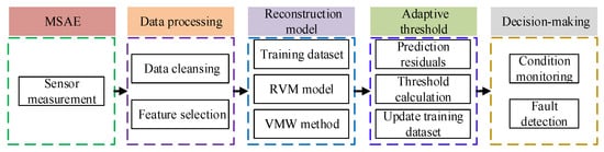
Figure 1.
Framework of the adaptive decision threshold.
The detailed calculation process of the adaptive threshold is as follows.
Step 1: The operation parameters of the MSAE were obtained. The data could be obtained directly from the ship alarm monitoring system (AMS).
Step 2: Data processing. Raw data cleansing and feature selection were necessary to extract meaningful and important information to avoid information redundancy.
Step 3: Data reconstruction. The RVM model was used to realize data reconstruction, and the VMW method was used to improve the reconstruction performance and realize continuous reconstruction.
Step 4: Residual calculation. The residual between the reconstruction values and the real-time observed measurement was calculated.
Step 5: Residual Gauss transformation by Johnson system. The residual data showed some unknown distribution. Most of the current threshold-setting methods are based on the assumption that a residual conforms to a normal distribution. Therefore, it was necessary to convert the prediction residual to normal and then determine the threshold.
Step 6: Adaptive threshold calculation. The training dataset was updated with real-time data, Steps 2–5 were repeated, and the adaptive threshold calculation was realized.
Step 7: Threshold application. According to the decision threshold, the abnormal diagnosis was realized, and the status monitoring and evaluation were realized by the degree of deviation in the state parameters from the baseline and threshold.
3. Methodology
The adaptive threshold fusion model is mainly composed of three parts. Firstly, the RVM method is applied to reconstruct data according to parameter correlation. Then, the residual probability distribution model is adopted to calculate the upper and lower thresholds. Finally, these thresholds adaptively update by the dynamic window and step size.
3.1. Data Processing
Most real data collected from the ship AMS are time-series data. Affected by the measurement uncertainty and complicated engine room environment, the data contain errors such as noise, bias, and outliers. Meanwhile, there will be data missing during data transmission. These abnormal data will lead to the wrong estimation of the system equipment performance. Therefore, data processing is crucial before the adaptive threshold calculation.
3.1.1. Raw Data Cleansing
Data imputation is the first step of the data processing process depending on a K nearest neighbors (KNN) approach [26]. The distance between the target dataset (data records containing missing items) and the complete dataset is denoted as . The Euclidean distance (Equation (1)) was selected as a distance metric to measure different attributes.
Data cleansing refers to the discovery and correction of identifiable errors in datasets. In the AMS, preprocessing the original data could avoid the influence of outliers on the threshold calculation and make the model calculation results more accurate. The isolation forest algorithm [27] can achieve efficient anomaly detection. Therefore, it is applied to the filtering of abnormal data.
3.1.2. Feature Selection
The Pearson correlation coefficient could be used to calculate the strength and direction of the correlation of parameters, thus reducing the complexity and computing time of the model [28]. According to this method, the absolute value of two signal correlation coefficients is between 0.3 and 0.5, which indicates that they have a certain correlation. If the absolute value is between 0.5 and 0.8, it indicates that there is a moderate correlation between signals. If the value is greater than 0.8, it indicates that there is a strong correlation between signals [29]. It can be considered that when the absolute value is greater than 0.5, one signal can more accurately reflect the change in another signal.
The correlation coefficient between the variables and is inducted by Equation (2).
where is the number of samples, and , represents the th values of the and , respectively, and , is the mean of the , , respectively. The correlation coefficient matrix of and is obtained as follows.
where is the training set sample dimension, is the correlation coefficient between and .
Through the correlation coefficient analysis, the relationship between the reconstructed signal and its associated signal was discovered. The measurement parameters with strong correlation were chosen to form the training set.
3.2. Reconstruction Model
The reconstruction model is the most important part of system condition monitoring and health management. In this study, the RVM is presented to establish the reconstruction model and the VMW method was used to improve the effect of reconstruction and realize continuous threshold calculation.
3.2.1. RVM Regression Prediction Model
The RVM adopted the same decision-making form as the SVM. For the given state parameter training dataset and independent target value, the RVM also adopted the same prediction function as the SVM.
where is the weight parameter vector, and sample noise , then . The input of the RVM model could be expressed by Equation (5).
where and N are the RBF kernel function and the number of training samples. Based on Equations (4) and (5), the hyperparameter was introduced. The likelihood function of the training sample could be written as shown in Equation (6).
where , is the design matrix.
If , then the basis function vector was .
As the ultimate goal of training the RVM prediction model was to find the posterior distribution of , it was assumed that . Then, the prior conditional probability distribution of was
where and each independent only corresponded to .
According to the Bayes formula, the posterior distribution formula of could be obtained by combining Equations (6) and (7).
where and obeyed a Gauss distribution. was not included in , so it could be regarded as a normalization coefficient, and the posterior distribution of could be expressed as
where .
As the hyperparameters and could directly affect the posterior distribution of , it was necessary to optimize the hyperparameters to obtain the maximum posterior distribution of . By maximizing the marginal likelihood function , we could optimize the hyperparameters. The objective function can be obtained by taking the negative logarithm of , then by making the partial derivative of the objective function with respect to the hyperparameters and to be zero, we can obtain
where is the posterior probability average weight of , , is the posterior weight covariance matrix obtained with Equation (10), and is the amount of sample data.
In the convergence process of hyperparameter estimation, an a posteriori probability distribution based on weight was used for prediction, and the limit condition was that and took the maximum value. If a new input value was given and the corresponding prediction target value was , then the probability distribution of the corresponding prediction output followed the Gaussian distribution:
where is the predicted value of .
3.2.2. Varying Moving Window Method
The moving window size affected the reconstruction performance of the RVM model, so a VMW method was proposed. The data in the window are treated as the training sample, while the step size is equal to the number of reconstruction data. At the end of each process, the data in the window are updated timely by the real-time data. Figure 2 illustrates the VMW method. represents the parameter information at the current time, is the window size, and is the sliding step. The size of and should be adjusted adaptively according to the actual situation.
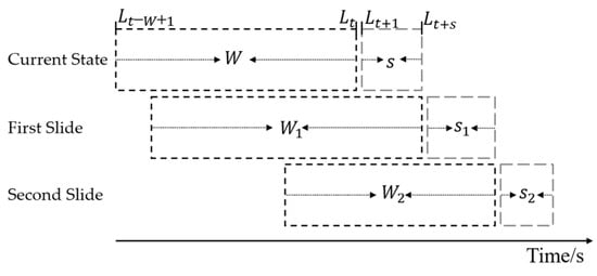
Figure 2.
VMW method.
In general, the window size should be large enough to cover enough samples for online modeling and reconstruction. A larger window size may contain more historical information for the RVM to track the changing trend of the state parameters but could not have the ability to accurately track abrupt changes. The small window size can usually reflect the rapid change in or mutation of the state parameters, but it may not contain enough information to fully reflect the operation status. Taking these factors into consideration, the window size should be a variable parameter that varies depending on data fluctuation. Thus, an adaptive updating method for a window size is proposed [30].
where and are the upper and lower limits of the window size, represents the Euclidean norm, represents the absolute value of the difference between two continuous variances of vectors and , and are the basic mean value and mean variance calculated by using historical data of the health stage. The window size will vary in the adjustment range and according to the parameter changes. is determined by autocorrelation analysis and is based on the trial-and-error method.
3.3. Adaptive Threshold Calculation
Johnson distribution systems were used to transform the residual data for the measurement and prediction into normal data [31]. The method established three families of distribution for the variable , which were , , and (the subscripts B, L, and U indicate that was bounded, lognormal, and unbounded, respectively). The three families of functions and the conditions to be satisfied are shown in Table 1. By using these functions, the data could be transformed into the standard normal distribution, and the distribution of the residual data after normalization is shown in Figure 3. The empirical probabilities of the transformed data points represented by blue + shown in (a) were near the red reference line, and the histogram of the frequency distribution of the transformed data points in (b) was very close to the red normal distribution curve. The results show that this method could successfully convert the residual data into a normal distribution.

Table 1.
Johnson distribution systems.
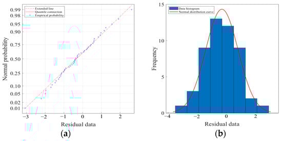
Figure 3.
Distribution of the residual data after normalization. (a) Normal probability diagram; (b) frequency distribution histogram.
After obtaining the transformed normal data, we could determine the calculation idea for the fixed threshold value. Firstly, according to the assumption that 95.45% of the normal distribution data fall in the region, the threshold of normal distribution could be determined (). Then, the threshold value of was calculated according to the formula in Table 1. For example, the threshold value calculation when selecting the method is shown in Equation (17).
Then, was substituted into Equation (17), and finally, the threshold value was obtained as follows.
where is the real data and is the reconstruction data.
The threshold calculation of the and distribution was similar to that of . The final threshold calculation formula was selected according to the actual parameter distribution. This method was used to obtain the upper and lower bounds of the adaptive threshold. To continuously evaluate the failure threshold at any time, we introduced the VMW method to realize the continuous calculation of the threshold. With the evolution of the equipment state, more and more observed data slid into the model to update the training dataset and different failure thresholds were yielded automatically.
4. Case Study
This section is devoted to describing how the proposed adaptive threshold method was demonstrated with real ship data. The data selected in this paper mainly come from the state parameters of the ship’s main propulsion diesel engine (as shown in Figure 4) and some relevant data come from the auxiliary system. For the state parameters of the MSAE, it was not necessary to adopt an adaptive threshold for all of the parameters. According to the characteristics of a real ship, parameters that could easily be affected by environmental temperatures, loads, and sea state changes were selected for the adaptive threshold calculation. These parameters were important indexes for evaluating the states of the MSAE.
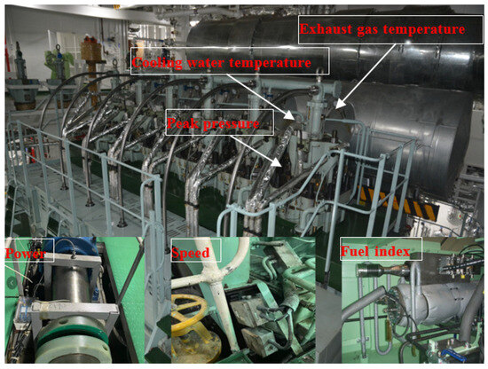
Figure 4.
System parameter acquisition.
4.1. Parameter Processing
4.1.1. Parameter Selection and Cleansing
As mentioned above, the peak pressure is the key parameter in the state parameters for a marine diesel engine. In particular, this parameter is used to evaluate the combustion performance of a diesel engine. It plays an important role in the decision-making of an autonomous system. Therefore, the peak pressure was selected as the research data, and the feasibility of the method was verified. Approximately 8000 data points from 1 January to 1 February 2019 were selected as the data samples for the threshold calculation. The distribution and change trends of the parameter points are shown in Figure 5. The value of the limits was the over-limit alarm threshold commonly used on the ship. This type of threshold is generally set by a factory. The peak pressure is stable and fluctuates within 1–7000 min. During the period of 7001 to end, the data decrease abnormally.
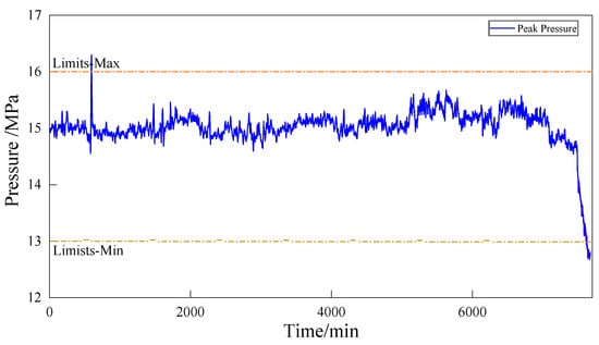
Figure 5.
Raw data of peak pressure.
The KNN and isolation forest algorithms were used to process the raw data. Figure 6 shows part of the time-series data for the peak pressure before and after the data processing. The denoised data are smoothed, following the trend of the raw data.
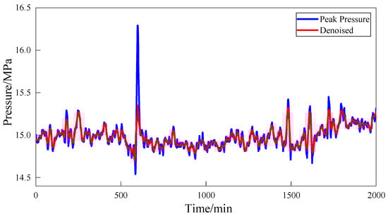
Figure 6.
Data cleaning.
4.1.2. Input Parameters Selection
There are many state parameters of an autonomous MSAE. In this paper, only the peak pressure and its related signal are selected for example analysis. Other relevant parameters of peak pressure are shown in Table 2.
Table 2.
AMS parameters for reconstruction model.
According to the Section 3.1.2 feature selection method, the correlation coefficients are calculated, and the results are shown in Figure 7. Table 3 shows the ranking of the correlation coefficient between each signal and peak pressure signal calculated by correlation analysis. If the absolute value of the correlation coefficient is greater than 0.5, then a given variable can predict other variables fairly accurately. Therefore, the first five features were selected as the input for the peak pressure reconstruction modeling.
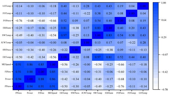
Figure 7.
Correlation coefficients for feature selection.
Table 3.
Correlation analysis between PPress and other parameters.
4.1.3. Determination of Window Size and Step Size
When the autocorrelation coefficient of the signal to be reconstructed is large, the corresponding window size is very small, which leads to the data in the window not being able to show the signal change trend, and it is easy to cause the overfitting of the reconstructed signal. However, an excessive window size results in an increase in the amount of calculation. Therefore, the is set at the point where the autocorrelation coefficient decreases gently. Figure 8 shows the autocorrelation analysis result of the PPress, the correlation coefficient decreases slowly after 200, so the is firstly set to 200.
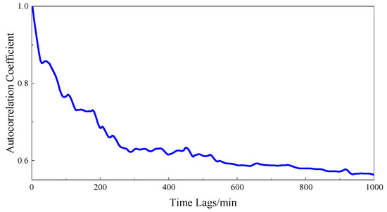
Figure 8.
Autocorrelation analysis results of state parameters.
According to the above method, the theoretical minimum window size is determined. The value of is used to quickly locate the window size. After the selection, the final parameters and are further selected according to the trial-and-error method [32]. Then, the optimal window selection is carried out within this window range. The mean absolute error (MAE) and root mean square error (RMSE) are used to evaluate the accuracy of the model, respectively, and the calculation time is employed to compare model efficiency. The VMW method determination steps are as follows.
Step 1: The theoretical is determined according to the method of autocorrelation analysis.
Step 2: A fixed window size is obtained at regular intervals near . The results of the autocorrelation analysis show that if the window size is too small, the data in the window will not fully reflect the changes in the equipment, and the model will be overfitted. Therefore, the too-small window size cannot be selected. After the above calculation, and the sizes of the fixed windows selected nearby are 100, 150, 200, 250, 300, 350, and 400.
Step 3: The above selected fixed window length is used for data reconstruction, and the three evaluation indexes of the MAE, RMSE, and calculation time are calculated. The calculation results are shown in Figure 9.
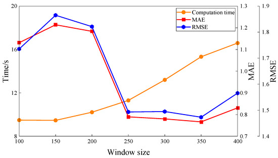
Figure 9.
Evaluation indexes and computation time under different window sizes.
Step 4: With the gradual increase in the window size, the time cost of the model is increasing, but the MAE and RMSE are decreasing. As a trade-off, the most appropriate window size is about 250. Usually, and should be distributed on both sides of this value. Therefore, set to 200 and set to 300 are the best choice.
Step 5: According to Equation (16), the adaptive calculation of the optimal window size is realized in and .
When the window size matrix is preset in step 2 and the weight is given to each index in step 3, the automatic setting of the window range would be realized.
The window sliding step could also be obtained by the trial-and-error method. The step size is expressed as a percentage of the window size. When the step size is 25% of the window size, it can balance the influence of the evaluation index and calculation time. So, in this paper, the window sliding step is set to 25% of the adaptive window size. According to the above calculation steps, the change in the dynamic window size and steps with time are shown in Figure 10.
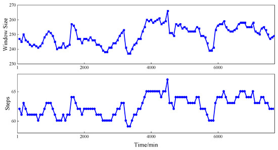
Figure 10.
Dynamic window size and steps with time.
4.2. Adaptive Threshold Calculation
4.2.1. Parameters Reconstruction
According to the characteristics of the peak pressure, the initial window size was determined by Equation (16). The sliding step size was selected as (rounded). The samples were used as the initial training set to reconstruct the peak pressure. The training data are updated (the number of updated data were equal to the step size), and the window and step size were recalculated. Therefore, the continuous reconstruction of the peak pressure data from to end was realized. Comparing the reconstructed values with the measured parameters, the reconstruction effect of a section of data is shown in Figure 11.
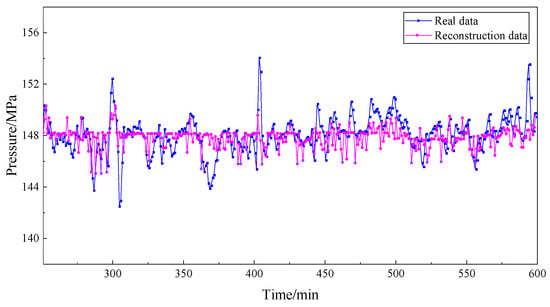
Figure 11.
RVM prediction effect for normal conditions.
The prediction effect of the VMW-RVM model was compared with those of the common SVM [25] and classical RVM prediction models. Three indicative indices, MAE, RMSE, and CPU running time (CPUT), are introduced in Table 4.
Table 4.
Comparison of the prediction accuracy.
It can be seen from Table 4 that the proposed method was better than the RVM and the SVM in terms of reconstruction accuracy. The proposed method could accurately describe the nonlinear and periodic changes in the parameters, so the model was a state parameter prediction method with a high prediction accuracy and reliable results. The threshold was time-dependent, and the time cost had to be considered in the model calculation. Illustrated by Table 4, the CPU time-consuming performance in the RVM method is better than the SVM’s.
4.2.2. Adaptive Threshold for Normal Condition
A section of the stable operation data was selected from the peak pressure data to test the effect of the adaptive threshold method in normal operation. As shown in Figure 12, the data from 4000 min to 5000 min were selected for analysis. It can be seen from the figure that the data were stably distributed between the upper and lower bounds of the threshold, the threshold bandwidth was narrow, the entire process is stable, and the upper and lower bounds were far from the limit value. If the limit value was selected as the reference for the alarm and state evaluation, early failures were not easy to detect.
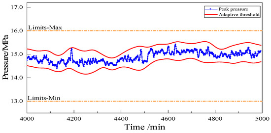
Figure 12.
Adaptive threshold for peak pressure (normal condition).
4.2.3. Adaptive Threshold for Abnormal Condition
A segment of abnormal data was selected from the peak pressure data to verify the adaptive threshold. As shown in Figure 13, the data from 6600 min to 7300 min were selected for analysis. These are the data of the abnormal peak pressure reduction caused by the fuel injector failure. It can be seen from the figure that T1, T2, and T3 indicate that the measurement parameter exceeded the adaptive threshold, , and the limit value, respectively. When there is a real fault, and the function of the system and equipment decreases significantly, an alarm will appear, which is an early warning. If the adaptive threshold was used as the alarm threshold, the early warning of a fault was achieved. In this way, enough time was spent on decision-making to prevent catastrophic accidents.
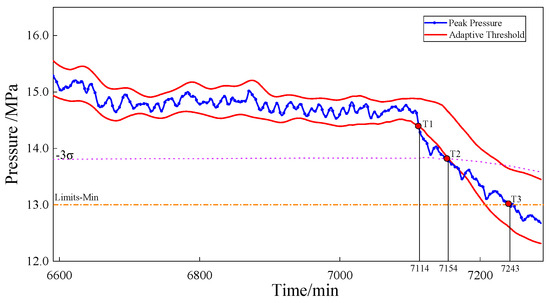
Figure 13.
Adaptive threshold for peak pressure (failure warning).
4.3. Results and Discussion
In the entire life cycle of the equipment, the threshold could be changed due to various factors. Compared with the fixed failure threshold shown in Table 5, the adaptive failure threshold was relatively flexible and convenient.
Table 5.
Different features of the traditional method and the proposed method.
Figure 14 illustrates the comparison between the adaptive threshold obtained using the RVM and SVM methods [25]. The exhaust gas temperature was applied to validate both the performances of the two approaches. From Figure 14, it is evident that the proposed strategy shows a more compact bandwidth, and meanwhile, the adaptive threshold obtained has better local adaptability, as shown in the area a. Both approaches can realize the early warning (167 min and 46 min) of the exhaust gas temperature (compared with the general limit value alarm method, the alarm time is T3). However, the threshold obtained by the RVM method is more sensitive to the data change trend, so it will trigger earlier fault warnings, as shown in T1. The parameters cross the threshold obtained by the SVM method at T2 and lag significantly. Therefore, the proposed adaptive threshold as the early warning threshold will have enough time to make appropriate decisions.
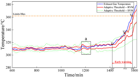
Figure 14.
Comparison of different reconstruction methods. The “a” box represents the comparison of threshold effects within a local area.
The deviation state evaluation method used the degree of deviation in the state parameters from the baseline and the threshold as the standard to measure the size of the health factors. As shown in Figure 15, the baseline was the optimal operation state for various operating conditions [33]. The area between the upper and lower bounds of the adaptive threshold was the most likely distribution area of the data. The area between the threshold and the limit value indicated that the data deviated from the main trend. Generally, an early warning had to be given to prevent further deterioration of the performance and a transition to a failure state. The baseline-adaptive threshold limits divided the equipment status into two levels: health status and subhealth status. If the real-time measurement parameter was between the baseline and the adaptive threshold, the equipment was in a healthy state, and the parameter value was calibrated for the deviation state of the threshold and the baseline to obtain the corresponding health value. If the parameter was between the threshold and the limits, it indicated that the equipment was in a sub-healthy state. This may have been due to degradation, condition changes, and other factors leading to performance changes. Combined with the remaining useful life (RUL) prediction algorithm, the health state prediction could be achieved.
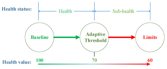
Figure 15.
Condition assessment.
Taking the above cases as examples, it can be seen that the adaptive threshold successfully detected the abnormalities and alarms in advance, and the threshold was more compact, flexible, and accurate in the entire process. This method overcame the disadvantage of the fixed threshold not being sensitive to the abnormal situation, improved the efficiency of the intelligent ship monitoring and alarm system, and provided more accurate data for the system state evaluation and auxiliary decision-making.
The adaptive threshold method detected the changes in the residual. Based on the premise that the residual was relatively stable, if the residual amplitude suddenly increased or decreased, that is, when a parameter deviated from the reference value due to an abnormality, the abnormal change could be detected successfully. However, if the abnormal changes were slow and significantly exceeded the ‘window’ size, the early warning could not be achieved with this method. At that time, it was necessary to combine the limit values to produce a fault alarm.
5. Conclusions
This article addressed the issues of an adaptive threshold in MSAE failure warning. Firstly, an innovative fusion model was proposed, which allowed considering the parameter processing, degradation uncertainty, and internal relations among the components. The reconstruction model was established based on the correlation of state parameters, and the residual probability distribution model was used to complete the threshold calculation. In addition, the threshold update was achieved by dynamically changing the window and step size according to the characteristics of the data changes. The adaptive threshold made the threshold bandwidth more compact locally, and it had a good effect on the tracking and identification of parameter change trends. Finally, the applicability and the performance of the proposed methodology for marine diesel engines were validated using data from the real ship AMS. In detail, this method was a trend monitoring method that could improve the accuracy of early warnings of MSAE failure. The obtained adaptive threshold could also be applied as a decision benchmark for condition assessment during the ship’s intelligent O&M process.
In this study, we considered slowly changing and single-mode MSAE state parameters with great inertia as the research object. For the system with multiple operation modes, different thresholds need to be determined according to different modes. Therefore, with the demand for a dynamic rapid-change and multimode system threshold calculation, the optimization of the algorithm will be further optimized in our future work.
Author Contributions
X.D. and Z.G. contributed equally to this work. Conceptualization, X.D. and Z.G.; methodology, Z.G. and P.Z.; software, Z.G. and Z.Q.; validation, Z.G. and Z.Q.; data curation, X.D. and T.D.; writing—original draft preparation, X.D. and Z.G.; writing—review and editing, T.D. and Y.Z. (Yongjiu Zou); supervision, Y.Z. (Yuewen Zhang) and P.S. All authors have read and agreed to the published version of the manuscript.
Funding
This research was funded by the National Key R&D Program of China (2022YFB4300805) and the Fundamental Research Funds for Central Universities (3132023525).
Institutional Review Board Statement
Not applicable.
Informed Consent Statement
Not applicable.
Data Availability Statement
Data is contained within the article.
Conflicts of Interest
Author Zhenxing Qiao was employed by the company Dalian Shipbuilding Industry Co., Ltd. The remaining authors declare that the research was conducted in the absence of any commercial or financial relationships that could be construed as a potential conflict of interest.
References
- Thieme, C.A.; Utne, I.B. Safety performance monitoring of autonomous marine systems. Reliab. Eng. Syst. Saf. 2017, 159, 264–275. [Google Scholar] [CrossRef]
- Hwang, H.J.; Lee, J.H.; Hwang, J.S.; Jun, H.B. A study of the development of a condition-based maintenance system for an LNG FPSO. Ocean Eng. 2018, 164, 604–615. [Google Scholar] [CrossRef]
- Zhang, P.; Gao, Z.; Cao, L.; Dong, F.; Zou, Y.; Wang, K.; Zhang, Y.; Sun, P. Marine Systems and Equipment Prognostics and Health Management: A Systematic Review from Health Condition Monitoring to Maintenance Strategy. Machines 2022, 10, 72. [Google Scholar] [CrossRef]
- Korun, M.; Vodenik, B.; Zorko, B. An alternative approach to the decision threshold. Appl. Radiat. Isot. 2018, 134, 56–58. [Google Scholar] [CrossRef] [PubMed]
- Lu, Y.; Sun, L.; Zhang, X.; Feng, F.; Kang, J.; Fu, G. Condition based maintenance optimization for offshore wind turbine considering opportunities based on neural network approach. Appl. Ocean. Res. 2018, 74, 69–79. [Google Scholar] [CrossRef]
- Aslansefat, K.; Bahar Gogani, M.; Kabir, S.; Shoorehdeli, M.A.; Yari, M. Performance evaluation and design for variable threshold alarm systems through semi-Markov process. ISA Trans. 2020, 97, 282–295. [Google Scholar] [CrossRef] [PubMed]
- Al-Dabbagh, A.W.; Hu, W.; Lai, S.; Chen, T.; Shah, S.L. Toward the Advancement of Decision Support Tools for Industrial Facilities: Addressing Operation Metrics, Visualization Plots, and Alarm Floods. IEEE Trans. Autom. Sci. Eng. 2018, 15, 1883–1896. [Google Scholar] [CrossRef]
- Izadi, I.; Shah, S.L.; Shook, D.S.; Chen, T. An Introduction to Alarm Analysis and Design. IFAC Proc. Vol. 2009, 42, 645–650. [Google Scholar] [CrossRef]
- Behrens, C.; Lopes, H.; Gamerman, D. Bayesian analysis of extreme events with threshold estimation. Stat. Model. 2003, 4, 227–244. [Google Scholar] [CrossRef]
- Bayarri, M.J.; Morales, J. Bayesian measures of surprise for outlier detection. J. Stat. Plan. Inference 2003, 111, 3–22. [Google Scholar] [CrossRef]
- Jablonski, A.; Barszcz, T.; Bielecka, M.; Breuhaus, P. Modeling of probability distribution functions for automatic threshold calculation in condition monitoring systems. Measurement 2013, 46, 727–738. [Google Scholar] [CrossRef]
- Wang, P.; Coit, D.W. Reliability and degradation modeling with random or uncertain failure threshold. In Proceedings of the 53rd Annual Reliability and Maintainability Symposium (RAMS), Orlando, FL, USA, 22–25 January 2007; pp. 392–397. [Google Scholar]
- Jin, X.H.; Sun, Y.; Que, Z.J.; Wang, Y.; Chow, T.W.S. Anomaly Detection and Fault Prognosis for Bearings. IEEE Trans. Instrum. Meas. 2016, 65, 2046–2054. [Google Scholar] [CrossRef]
- Liu, K.; Huang, S. Integration of Data Fusion Methodology and Degradation Modeling Process to Improve Prognostics. IEEE Trans. Autom. Sci. Eng. 2016, 13, 344–354. [Google Scholar] [CrossRef]
- Yazdinejad, A.; Dehghantanha, A.; Srivastava, G.; Karimipour, H.; Parizi, R.M. Hybrid Privacy Preserving Federated Learning Against Irregular Users in Next-Generation Internet of Things. J. Syst. Archit. 2024, 148, 103088. [Google Scholar] [CrossRef]
- Witczak, M.; Korbicz, J.; Mrugalski, M.; Patton, R.J. A GMDH neural network-based approach to robust fault diagnosis: Application to the DAMADICS benchmark problem. Control Eng. Pract. 2006, 14, 671–683. [Google Scholar] [CrossRef]
- Sun, Y.; Han, A.; Hong, Y.; Wang, S. Threshold autoregressive models for interval-valued time series data. J. Econom. 2018, 206, 414–446. [Google Scholar] [CrossRef]
- Jia, Q.; Chen, C.; Gao, X.; Li, X.; Yan, B.; Ai, G.; Li, J.-I.; Xu, J. Anomaly detection method using center offset measurement based on leverage principle. Knowl. Based Syst. 2020, 190, 105191. [Google Scholar] [CrossRef]
- Aminzadeh, M.; Kurfess, T. Automatic thresholding for defect detection by background histogram mode extents. J. Manuf. Syst. 2015, 37, 83–92. [Google Scholar] [CrossRef]
- Yousefi, N.; Coit, D.W.; Song, S.; Feng, Q. Optimization of on-condition thresholds for a system of degrading components with competing dependent failure processes. Reliab. Eng. Syst. Saf. 2019, 192, 106547. [Google Scholar] [CrossRef]
- Xu, X.; Li, S.; Song, X.; Wen, C.; Xu, D. The optimal design of industrial alarm systems based on evidence theory. Control Eng. Pract. 2016, 46, 142–156. [Google Scholar] [CrossRef]
- Louen, C.; Ding, S.X. Distribution independent threshold setting based on one-class support vector machine. IFAC-Pap. 2020, 53, 11307–11312. [Google Scholar] [CrossRef]
- Amirkhani, S.; Chaibakhsh, A.; Ghaffari, A. Nonlinear robust fault diagnosis of power plant gas turbine using Monte Carlo-based adaptive threshold approach. ISA Trans. 2020, 100, 171–184. [Google Scholar] [CrossRef] [PubMed]
- Cao, W.; Dong, G.; Xie, Y.-B.; Peng, Z. Prediction of wear trend of engines via on-line wear debris monitoring. Tribol. Int. 2018, 120, 510–519. [Google Scholar] [CrossRef]
- Yang, C.; Liu, J.; Zeng, Y.; Xie, G. Real-time condition monitoring and fault detection of components based on machine-learning reconstruction model. Renew. Energy 2019, 133, 433–441. [Google Scholar] [CrossRef]
- Murti, D.M.P.; Pujianto, U.; Wibawa, A.P.; Akbar, M.I. K-Nearest Neighbor (K-NN) based Missing Data Imputation. In Proceedings of the 2019 5th International Conference on Science in Information Technology (ICSITech), Yogyakarta, Indonesia, 23–24 October 2019; pp. 83–88. [Google Scholar]
- Lesouple, J.; Baudoin, C.; Spigai, M.; Tourneret, J.-Y. Generalized isolation forest for anomaly detection. Pattern Recognit. Lett. 2021, 149, 109–119. [Google Scholar] [CrossRef]
- Gao, H.; Liu, F.; Zhu, Q. A correlation consistency based multivariate alarm thresholds optimization approach. ISA Trans. 2016, 65, 37–43. [Google Scholar] [CrossRef] [PubMed]
- Yoo, Y. Data-driven fault detection process using correlation based clustering. Comput. Ind. 2020, 122, 103279. [Google Scholar] [CrossRef]
- Yu, J. State of health prediction of lithium-ion batteries: Multiscale logic regression and Gaussian process regression ensemble. Reliab. Eng. Syst. Saf. 2018, 174, 82–95. [Google Scholar] [CrossRef]
- Slifker, J.F.; Shapiro, S.S. The Johnson System: Selection and Parameter Estimation. Technometrics 1980, 22, 239–246. [Google Scholar] [CrossRef]
- Wang, L.; Yang, C.; Sun, Y.; Zhang, H.; Li, M. Effective variable selection and moving window HMM-based approach for iron-making process monitoring. J. Process Control 2018, 68, 86–95. [Google Scholar] [CrossRef]
- Zhang, P.; Sun, P.; Zhang, Y.; Jiang, X. Adaptive baseline model for autonomous marine equipment and systems. ISA Trans. 2021, 112, 326–336. [Google Scholar] [CrossRef] [PubMed]
Disclaimer/Publisher’s Note: The statements, opinions and data contained in all publications are solely those of the individual author(s) and contributor(s) and not of MDPI and/or the editor(s). MDPI and/or the editor(s) disclaim responsibility for any injury to people or property resulting from any ideas, methods, instructions or products referred to in the content. |
© 2024 by the authors. Licensee MDPI, Basel, Switzerland. This article is an open access article distributed under the terms and conditions of the Creative Commons Attribution (CC BY) license (https://creativecommons.org/licenses/by/4.0/).