Multivariate USV Motion Prediction Method Based on a Temporal Attention Weighted TCN-Bi-LSTM Model

Abstract

Unmanned surface vehicle (USV)’s motion is represented by time-series data that exhibit highly nonlinear and non-stationary features, significantly influenced by environmental factors, such as wind speed and waves, when sailing on the sea. The accurate prediction of USV motion, particularly crucial parameters, such as the roll angle and pitch angle, is imperative for ensuring safe navigation. However, traditional and single prediction models often struggle with low accuracy and fail to capture the intricate spatial–temporal dependencies among multiple input variables. To address these limitations, this paper proposes a prediction approach integrating temporal convolutional network (TCN) and bi-directional long short-term memory network (Bi-LSTM) models, augmented with a temporal pattern attention (TPA) mechanism, termed the TCN-Bi-LSTM-TPA (TBT) USV motion predictor. This hybrid model effectively combines the strengths of TCN and Bi-LSTM architectures to extract long-term temporal features and bi-directional dependencies. The introduction of the TPA mechanism enhances the model’s capability to extract spatial information, crucial for understanding the intricate interplay of various motion data. By integrating the features extracted by TCN with the output of the attention mechanism, the model incorporates additional contextual information, thereby improving prediction accuracy. To evaluate the performance of the proposed model, we conducted experiments using real USV motion data and calculated four evaluation metrics: mean square error (MSE), mean absolute error (MAE), mean absolute percentage error (MAPE), and R-squared (R²). The results demonstrate the superior accuracy of the TCN-Bi-LSTM-TPA hybrid model in predicting USV roll angle and pitch angle, validating its effectiveness in addressing the challenges of multivariate USV motion prediction.

1. Introduction

For unmanned surface vehicles (USVs), navigation safety is crucial to effectively fulfill their role in various tasks and plays an important role in ensuring the stability and safety of boats. Therefore, it is necessary to analyze the safe navigation status of USVs, which involves predicting motion data in advance. In this context, the accurate prediction of USV motion is essential for promptly assessing the status of USVs and implementing proactive control measures based on the prediction outcomes. This will significantly enhance the seaworthiness and safety of USVs [1,2]. Due to the complexity and unpredictability of sea conditions, when USVs sail on the sea, they often experience the coupling effects of multiple factors, such as winds, waves, and currents [3,4]. Therefore, the high-precision prediction of USV motion is quite challenging. The complex environment results in complex nonlinear six-degree-of-freedom random motion, including roll, pitch, yaw, sway, surge, and heave. In this six-degree-of-freedom motion, the roll angle and pitch angle are closely related to the sailing stability of USVs [5]. If these angles are too large, the possibility of capsizing increases.

The current research on USV motion prediction can be categorized into three main methods: mathematical models, statistical models, and machine learning models. The prediction methods based on the mathematical model involve establishing a mathematical model of the ship’s motion and the surrounding marine environment. The more typical methods include the Kalman filter method [6], as well as the bow wave method [7]. It is worth noting that, although such methods have natural advantages in the interpretability of forecasts, they often rely on a large number of empirical formulas, leading to the accuracy of forecasts being highly affected by environmental factors and often failing to meet real-time forecasting requirements [8].

Statistical prediction methods are primarily based on regression analysis. These methods treat the ship’s motion attitude data as a sequence of random variables arranged in chronological order, including autoregressive (AR) models, autoregressive moving average (ARMA), and autoregressive integrated moving average (ARIMA). In [9], researchers introduced an AR model combined with error correction, aiming to minimize errors in the iterative process and improve the accuracy of multi-step predictions. In [10], the ARMA model was used to predict ship motion attitude data and achieved a better prediction performance than the AR model. While the ARMA model is effective in handling prediction errors, it requires stationary data to produce accurate results, which restricts its applicability. The ARIMA model incorporates differencing based on the ARMA model, which transforms non-stationary external datum into stationary datum before inputting it into the ARMA model. In [11], researchers utilized the ARIMA model to rectify prediction errors, leading to enhanced prediction accuracy by employing a single prediction method. Although their performance is gradually improving, these models are linear methods and limited in their ability to handle the strong nonlinearity of motion attitude data generated in complex ocean environments.

To better deal with the characteristics of nonlinear and non-stationary inputs caused by rough sea state and hydrodynamic factors, motion prediction methods based on machine learning models have emerged. The research on using machine learning theoretical-based methods can be divided into two categories: methods based on traditional machine learning models and methods based on deep learning models. For the former, scholars mostly use support vector regression (SVR) and decision tree (DT) methods. In [12], the empirical mode decomposition (EMD) method was used to preprocess the raw data and input them into an SVR model to mitigate the marginal effect of EMD and generate short-term forecasts of ship movements. With the development of DT methods, some variant models are utilized for prediction, such as random forest (RF) and eXtreme gradient boosting (XGBoost). In [13], the researchers combined a traditional data-driven model with the RF model to develop a ship-speed prediction model, resulting in higher accuracy and applicability compared to traditional prediction models that only consider environmental factors as features. In order to address the issue of the inadequate prediction accuracy of a single XGBoost model, a combined prediction model using XGBoost and a convolutional long short-term memory neural network (Conv-LSTM) was proposed [14], and an accurate prediction model was created by training the two models independently and then combining them.

Due to the ability to adapt to complex patterns, better generalization, and sufficient scalability, deep learning methods based on artificial neural networks have become a popular research direction in the field of predicting ship motion data. This approach commonly employs USV motion data as time-series inputs and utilizes diverse time-series prediction models to forecast USV motion data. It can learn nonlinear features in a large amount of input data through nonlinear activation functions. Note that current studies on predicting ship motion data using artificial neural networks are mainly based on recurrent neural network (RNN) [15] and convolutional neural network (CNN) models [16]. For research based on the RNN method, LSTM [17] and GRU [18] are widely used. In [19], researchers proposed a theory-driven and data-driven approach combined model and utilized LSTM to formulate a ship-following behavior prediction model. In [20], LSTM and gated recurrent unit (GRU) models were reconstructed, and the researchers incorporated residual connections into the standard architecture and achieved high-accuracy real-time predictions. Some scholars utilized bi-directional recurrent neural network models, including Bi-LSTM, bi-directional convolution long short-term (Bi-Conv-LSTM), and bi-directional gated recurrent unit (Bi-GRU), to enhance the extraction of features from the input data. In [21,22], Bi-LSTM was utilized for forecasting ship roll attitude data and demonstrated that the bi-directional structure of the LSTM model outperformed the unidirectional structure. In [23], researchers proposed a channel attention-weighted Bi-Conv-LSTM hybrid model for ship pitch angle predictions, and achieved high-precision forecasting on specific datasets. And, in [24], the BIGRU model was utilized for predicting the trajectory of ship motion by integrating an efficient channel attention mechanism, and the performance of the model under different iterations was analyzed.

Due to the advantages of weight sharing and low computational resource consumption, CNN-based methods are increasingly being utilized in the field of ship motion prediction. Based on the powerful feature extraction capability of the CNN, more and more researchers tend to combine CNN and RNN methods for ship motion predictions, achieving the ability to extract multi-modal information in time and space at the same time. In [25], researchers designed a new structure for a RNN-based model to capture the spatial features handled by the CNN model. Zhang et al. [26] combined a CNN with LSTM to establish a ship roll attitude prediction model, using the CNN to extract the spatial features of input data and LSTM to extract temporal features. Wei et al. [27] established a prediction model based on CNN and Bi-LSTM models, which performed bi-directional feature extraction on the basis of CNN-LSTM, and compared it with other models, such as SVR, DBN, and ARMA. to verify the effectiveness of the proposed algorithm. In [28], unlike previous work, the researchers built a hybrid model by adding a CNN to the back of a Bi-LSTM model to extract the bi-directional cross-temporal features of inputs, and established two high-precision prediction models for single-variable and multi-variable input scenarios. There are also some researchers who combined a CNN with GRU; Rashid et al. [29] and Li et al. [30] chose to combine a CNN and GRU to simplify the computational complexity of the LSTM model, and their work proved that the GRU model combined with a CNN shows a good performance in the task of predicting ship motion attitude data, and is better than the single GRU model in model training.

In order to leverage convolutional neural network (CNN) models for capturing temporal patterns in time-series data, a model known as the temporal convolutional network (TCN) was proposed [31]. The TCN makes use of stacked residual connection blocks consisting of one-dimensional dilated causal convolutions to effectively extend the receptive field of the model. This extension enables the model to capture and model complex temporal relationships within the time-series data. By incorporating dilated convolutions, the TCN can efficiently capture long-range dependencies in the temporal domain and extract meaningful features from time-series inputs. The utilization of residual connections helps alleviate the vanishing gradient problem and allows for the more effective and stable training of the network. By taking advantage of both dilated convolutions and residual connections, the TCN has demonstrated a promising performance in forecasting. In [32], the researchers combined the TCN model with variational modal decomposition (VMD) and proposed a novel prediction model; this model utilized the TCN to process ship motion data after decomposition and performed high-precision predictions. In [33], the researchers employed the TCN model to determine the optimal hyper-parameters in conjunction with the optimization algorithm and developed a prediction model suitable for various sea states. Due to the excellent ability of the TCN to capture temporal features, there are many studies that combine them with RNN models to comprehensively improve the prediction ability of the models. In [34], the researchers proposed a parallel architecture model based on TCN-LSTM and investigated such a combined model for wind power prediction, and the results show that the proposed model performs better in terms of prediction performance and generalization and has a faster convergence speed compared with the separate prediction model and the serial model of TCN-LSTM. Some scholars [35] combined a TCN and Bi-GRU for generator capacity prediction and assigned capacity weights to different distribution modes through the attention mechanism to improve the accuracy of prediction. In comparison with traditional machine learning and deep learning prediction models, the proposed prediction method has a higher capacity accuracy inspired by bi-directional recurrent class neural networks. In [36], the researchers employed a combination of the TCN model and Bi-LSTM in their study. In addition, the researchers integrated the complete ensemble empirical mode decomposition with adaptive noise (CEEMDAN) and empirical wavelet transform (EWT) decompositions into the model to decompose the input data so that the model could be targeted for predictions based on different decomposition features. The proposed model’s performance was thoroughly evaluated through extensive comparative experiments. These experiments provided a robust validation and assessment of the model’s effectiveness in handling time-series data.

For USV motion prediction, many existing studies primarily focus on univariate features or neglect the interplay between different motion data variables of USVs. However, due to the complex and non-linear nature of USV motion data, insufficient consideration of the spatial relationships between USV motion data variables often hinders the accuracy of the predictions [37]. To overcome these limitations, this study proposes a method based on the TCN-Bi-LSTM-TPA hybrid model to enhance the accuracy of USV motion predictions in multivariate scenarios. The contributions and motivations of this paper can be summarized as follows:

• Aiming to capture the sequence characteristics and inter-dependencies among multivariate USV motion inputs, this research considers multiple variables input simultaneously by establishing spatial–temporal mapping relationships among multiple USV features.
• To effectively extract temporal features from USV motion data, this paper integrates TCN and Bi-LSTM models. By leveraging the strengths of these models, the proposed methodology can capture long-term dependencies and bi-directional causal relationships, enabling more accurate prediction results.
• In order to address the coupling effect between different motion data variables, this research enhances the model’s ability to process spatial information through the TPA mechanism. Additionally, Conv-1D is used at the end of the model to extract local spatial features to further enhance the prediction accuracy.
• Numerical experiments are conducted using the roll and pitch motion data of an actual USV to verify the feasibility and effectiveness of the proposed model compared with nine established classic prediction models.

The remaining structure of the paper is described as follows: Section 2 introduces the neural network structure used in this study; Section 3 describes research methodology, including the proposed prediction model’s structure and the methods used to train the model and generate predictive values; Section 4 shows the data description and experimental results; Section 5 discusses the experimental results; and Section 6 summarizes the conclusions and discusses future work.

2. USV Motion Feature Extraction Structure

2.1. TCN Nerual Network

This paper utilizes dilated causal convolution to construct a TCN neural network aimed at effectively capturing long-term temporal trends from input data. By employing dilated causal convolutions, the network is capable of significantly increasing the receptive field size through the deepening of layers.

In traditional convolutional neural networks, the receptive field size exhibits a linear growth pattern in correlation with the network depth and the size of the convolutional kernel. For instance, considering a convolutional neural network with n-layer 1D convolutional layers, each equipped with a kernel size of k, the receptive field, r, can be calculated as follows:

$$r=1+n·(k-1)$$

(1)

It is evident that producing a large receptive field in traditional convolutional neural networks can be accomplished by either increasing the size of the convolutional kernel or adding more convolutional layers. However, these approaches may lead to excessively deep network architectures, which can introduce challenges such as gradient vanishing or exploding. Moreover, the increased model complexity can result in higher training costs. Therefore, in this paper, dilated casual convolution was utilized to create a larger receptive field while mitigating the issue of excessively deep network layers. Dilated causal convolution is introduced to manage the exponential expansion of the convolution kernel as the number of network layers increases, for instance, considering a convolutional neural network with a 1D dilated causal convolutional layer. When setting the initial dilation factor to d and the initial convolutional kernel size to k, then the output layer’s receptive field of the network can be calculated as follows:

$$r=1+\frac{(k-1)(d^n-1)}{d-1}$$

(2)

where n is the number of dilated causal convolutional layers; by adjusting the values of d and k, the receptive field can be significantly enlarged without requiring an excessively deep network architecture. This approach allows us to capture long-term temporal patterns in the input data while maintaining a manageable network depth. Assuming a given one-dimensional input sequence, ${\mathit{X}}_{1,T }=\left\{x_1, x_2, \cdots ,{ x}_T\right\}\in {\mathbb{R}}^{1\times \mathrm{T}}$, and an n-dimensional convolution filter, $\mathit{k} = \{k_0,{ k}_1, \cdots ,{ k}_{\mathrm{n}}\}\in {\mathbb{R}}^{1\times n}$, the result of the dilated causal convolution at time step t can be represented by Equation (3) [31]:

$$\mathit{X}\ast {\mathit{k}}_t={\displaystyle \sum _{s=0}^{n-1}{\mathit{k}}_s{\mathit{X}}_{t-d\times s}}$$

(3)

As opposed to RNN-based models, the TCN offers the advantage of analyzing longer sequence inputs. This characteristic is beneficial for parallel computing, model simplification, and the prevention of gradient explosions. By stacking residual layers, computational resources can be conserved while simultaneously expanding the network’s receptive field and capturing longer input sequences. The structure of the TCN neural network is illustrated in Figure 1.

2.2. LSTM and Bi-LSTM Neural Networks

The traditional recurrent neural network often encounters the issue of gradient vanishing when processing temporal information. To address this problem, LSTM was introduced. Building on the foundation of traditional a RNN, the LSTM network incorporates gating units to regulate the flow and retention of information. It consists of three gates, the input gate, output gate, and forget gate, which determine whether the hidden state of the current time step should be passed along to the next step. This design effectively circumvents the gradient vanishing problem associated with traditional RNNs and enables the capture of sequence feature information over longer time steps.

When the LSTM network processes time-series data, the data of the current time step are only determined by the sequence of the earlier time steps; so, the transmission of its hidden state follows a unidirectional flow from front to back. Based on the LSTM network, the Bi-LSTM network incorporates a bi-directional design. This design increases the hidden layers transmitted from front to back. Consequently, when the hidden state is transmitted, in addition to the front-to-back transmission, it will also be transmitted from the back to the front, and its structure is shown in Figure 2.

Assuming that ${\mathit{x}}_t\in {\mathbb{R}}^{n\times 1}$ is the USV motion feature that input into Bi-LSTM at the t time step, n is the number of samples. In Figure 2, ${\overrightarrow{\mathit{h}}}_t\in {\mathbb{R}}^{h\times 1}$ represents the forward-propagation hidden state, while ${\overleftarrow{\mathit{h}}}_{\mathrm{t}}\in {\mathbb{R}}^{h\times 1}$ represents the backward-propagation hidden state, where h is the number of forward and backward hidden units. Then the forward and backward hidden states output of the Bi-LSTM, ${\mathit{h}}_t \in {\mathbb{R}}^{h\times 1}$, is computed by Equations (4)–(6):

$${\overrightarrow{\mathit{h}}}_t={\overrightarrow{\mathit{o}}}_t\odot tanh({\overrightarrow{c}}_t)$$

(4)

$${\overleftarrow{\mathit{h}}}_t={\overleftarrow{\mathit{o}}}_t\odot tanh({\overleftarrow{c}}_t)$$

(5)

$${\mathit{h}}_t=concat({\overrightarrow{\mathit{h}}}_t,{\overleftarrow{\mathit{h}}}_t)$$

(6)

where $⨀$ denotes the product of the elemental direction; ${\overrightarrow{\mathit{o}}}_t$ and ${\overleftarrow{\mathit{o}}}_t$ denote the outputs of the forward and backward LSTM output gates at the t time step, respectively (they are calculated in the same way, as shown in Equation (9)); and the other two gates, the forget gate and input gate, can be calculated as Equations (7) and (8) [17]. ${\overrightarrow{\mathit{c}}}_t$ and ${\overleftarrow{\mathit{c}}}_t$ denote the memory cell outputs of the forward and backward LSTM inputs at the t time step, respectively, which are also calculated in the same way, as shown in Equation (11). The function tanh is the activation function applied to the memory cell.

$${\mathit{f}}_t=\sigma ({\mathit{W}}^{(f)}\cdot {[{\mathit{x}}_t,{\mathit{h}}_{t-1}]}^T+{\mathit{b}}_f)$$

(7)

$${\mathit{i}}_t=\sigma ({\mathit{W}}^{(i)}\cdot {[{\mathit{x}}_t,{\mathit{h}}_{t-1}]}^T+{\mathit{b}}_i)$$

(8)

$${\mathit{o}}_t=\sigma ({\mathit{W}}^{(o)}\cdot {[{\mathit{x}}_t,{\mathit{h}}_{t-1}]}^T+{\mathit{b}}_o)$$

(9)

$${\tilde{\mathit{c}}}_t=tanh({\mathit{W}}^{(\tilde{c})}\cdot {[{\mathit{x}}_t,{\mathit{h}}_{t-1}]}^T+{\mathit{b}}_{\tilde{c}})$$

(10)

$${\mathit{c}}_t={\mathit{f}}_t\odot {\mathit{c}}_{t-1}+{\mathit{i}}_t\odot {\tilde{\mathit{c}}}_t$$

(11)

where ${\tilde{\mathit{c}}}_t$ indicates the candidate memory cell output, which can be calculated as Equation (10). ${\mathit{W}}^{\left(f\right)}$ consists of ${\mathit{W}}_{\mathit{xf}}\in {\mathbb{R}}^{h\times 1}$ and ${\mathit{W}}_{\mathit{hf}}\in {\mathbb{R}}^{h\times h}$, which represent the weights multiplied by the input and multiplied by the hidden state of the forget gate, respectively; ${\mathit{W}}^{\left(i\right)}$ consists of ${\mathit{W}}_{\mathit{xi}}\in {\mathbb{R}}^{h\times 1}$ and ${\mathit{W}}_{\mathit{hi}}\in {\mathbb{R}}^{h\times 1}$; ${\mathit{W}}^{\left(o\right)}$ consists of ${\mathit{W}}_{\mathit{xo}}\in {\mathbb{R}}^{h\times 1}$ and ${\mathit{W}}_{\mathit{ho}}\in {\mathbb{R}}^{h\times 1}$; and ${\mathit{W}}^{\left(\tilde{c}\right)}$ consists of ${\mathit{W}}_{x\tilde{c}}\in {\mathbb{R}}^{h\times 1}$ and ${\mathit{W}}_{h\tilde{c}}\in {\mathbb{R}}^{h\times 1}$. Then, ${\mathit{b}}_f$, ${\mathit{b}}_i$, ${\mathit{b}}_o$, and ${\mathit{b}}_{\tilde{c}}$ represent the corresponding bias terms of different information units, and $\sigma$ denotes the activation function.

2.3. Temporal Pattern Attention Mechanism

As deep learning has advanced, the attention mechanism was introduced to capture the hidden and diverse information in deep learning models. The TPA mechanism [38] is specially designed for time-series data. To retain the temporal pattern when extracting spatial features, the TPA mechanism uses a convolutional filter to extract the fixed-length time-series mode from the input information; then, it employs a scoring function to determine the appropriate weight of each time-series mode to extract spatial features. Finally, the output information is obtained based on the values of weights. Unlike the traditional attention mechanism, which primarily emphasizes the relationship between the features of the input data, the TPA mechanism goes a step further by considering the temporal relationship in addition to the spatial relationship. It assigns weights to the features of each time step of the input data to calculate the weights at different time steps. For the TCN-Bi-LSTM-TPA hybrid model proposed in this paper, the inputs to the TPA mechanism are temporal features for several time steps processed by the residual TCN-Bi-LSTM framework. Its scheme is illustrated in Figure 3.

In Figure 3, assuming that $\mathit{H}=[{\mathit{h}}_{t-w}{, \mathit{h}}_{t-\left(w-1\right)},\cdots ,{ \mathit{h}}_t]$ represents the output hidden states of previous model’s outputs, ${\mathit{C}}_j$ denotes the convolution kernel and w is the predetermined number of time steps to be predicted. The result of the calculation is denoted as ${ \mathit{H}}_{i,j}^C$, where subscripts i and j, respectively, represent the data selected in the i-th row and j-th column for the convolution operation. The final output of the TPA mechanism is computed by Equations (12)–(16):

$${\mathit{H}}_{i,j}^C={\displaystyle \sum _{i=1}^W{\mathit{H}}_{i,(t-w-1+l)}\times {\mathit{C}}_{j,T-w+l}}$$

(12)

$$f\left({\mathit{H}}_i^C,{\mathit{h}}_t\right)={\left({\mathit{H}}_i^C\right)}^T{\mathit{W}}_a{\mathit{h}}_t$$

(13)

where T represents the maximum weight extracted by the convolution kernel, which is often taken as w. l is the filling length in the convolution operation. f is the score function used to compute the attention weights, which is shown in Equation (14):

$${\mathit{a}}_i=\sigma \left(f\left({\mathit{H}}_i^C,{\mathit{h}}_t\right)\right)$$

(14)

where ${\mathit{a}}_i$ represents the weight of the TPA and $\mathsf{\sigma }$ represents sigmoid, which is used as the activation function of the weight matrix calculation. After obtaining the convolution values and weights, attention vector ${\mathit{v}}_t$ can be calculated as:

$${\mathit{v}}_t={\displaystyle \sum _{i=1}^n{\mathit{a}}_i{\mathit{H}}_i^C}$$

(15)

Then add the hidden state ${\mathit{h}}_t$ and the attention vector ${\mathit{v}}_t$ after the linear mapping operation to obtain the predicted value ${\mathit{y}}_t$ of the output model, which is shown in Equation (16), where ${\mathit{W}}_y$, ${\mathit{W}}_h$, and ${\mathit{W}}_v$ denote the corresponding weights:

$${\mathit{y}}_t={\mathit{W}}_y({\mathit{W}}_h{\mathit{h}}_t+{\mathit{W}}_v{\mathit{v}}_t)$$

(16)

3. Methodology

3.1. The Scheme of Predicted Values’ Generation and Model Training

The multivariate motion data of the USV can be regarded as a series of multi-dimensional time-series data, including the roll angle, pitch angle, rotation rate, heading angle, and other related variables. In this paper, the USV motion prediction problem is regarded as a regression task with supervised learning, so it is necessary to construct USV motion data in the form of data with samples and labels, which are usually implemented by using a sliding window, as shown in Figure 4.

In Figure 4, the sliding window divides the multivariate input USV motion into sample data (indicated by the gray dots) and label data (indicated by the green dots). For the sample data, assuming that the USV motion dataset consists of N variables and T time steps are sampled together, then the dimension is 1, and USV motion data from the preliminary sampling time step t-T to the current moment, t, can be expressed as ${ \mathit{X}}_{t-T:t}=\left\{x_{t-T},x_{t-(T-1)},\cdots ,x_t\right\}\in {\mathbb{R}}^{\mathrm{T}}$. Thus, the multivariate USV motion data ${\mathit{X}}_{1:N,t-T:t }\in {\mathbb{R}}^{N\times T}$ with a dimension of N and a sampling time step of T can be expressed as ${\mathit{X}}_{1:N,t-T:t }=\left\{{\mathit{X}}_{1,t-T:t},\cdots {,\mathit{X}}_{i,t-T:t},\cdots ,{\mathit{X}}_{N,t-T:t}\right\}\in {\mathbb{R}}^{N\times T}$, where ${\mathit{X}}_{i, t-T:t }\in {\mathbb{R}}^T$ denotes the time-series data from time step t-T to time step t of the i-th dimension.

For the label data, since the sliding window only moves one step at a time and only generates label data at the following moment each time, let P represent the total sliding step size of the sliding window; thus, label data ${ \mathit{Y}}_{1:N,t;t+P }\in {\mathbb{R}}^{N\times P}$ can be generated by iteratively moving the sliding window, as shown in Figure 4. Therefore, the prediction of USV motion data uses the historical time-series data input ${\mathit{X}}_{1:N,t-T:t }\in {\mathbb{R}}^{N\times T}$ to predict the trend change in the data in future P time steps, which is presented as ${\widehat{\mathit{Y}}}_{1:N,t;t+P }\in {\mathbb{R}}^{N\times P}$.

Assuming that there is a mapping relationship of $f_{\Theta }(·)$ from ${\mathit{X}}_{1:N,t-T:t }$ to ${\widehat{\mathit{Y}}}_{1:N,t;t+P }$, the training problem of the USV motion prediction model can be abstracted to find a suitable parameter matrix, $\theta$, so that the error between the historical observation data of the USV motion data and the predicted data obtained through mapping $f_{\theta }(·)$ is minimized, and this process can be expressed as shown in Equation (17):

$$\begin{array}{l}\underset{\Theta }{min}{L}_f({\stackrel{⌢}{\mathit{Y}}}_{1:N,t:t+P},{\mathit{Y}}_{1:N,t:t+P})\\ s.t.{\stackrel{⌢}{\mathit{Y}}}_{1:N,t+P}={\mathit{f}}_{\mathit{\Theta }}({\mathit{X}}_{1:N,t-T:t})\end{array}$$

(17)

where $L_f$ represents the loss function between the predicted value, ${\widehat{\mathit{Y}}}_i$, and the true value, ${\mathit{Y}}_i$, which can be expressed as:

$$L_f=\frac{1}{n}{\displaystyle \sum _{i=1}^n({\stackrel{⌢}{\mathit{Y}}}_i-{\mathit{Y}}_i)}$$

(18)

where n is the number of samples. Figure 5 shows the overall flowchart of the TBT USV motion prediction model. In Figure 5, the process can be summarized as follows:

• USV motion data preprocessing: The sliding window technique is utilized for obtaining multivariate USV motion data as inputs. The input data undergo preprocessing, which includes data normalization and data splitting, to meet the input and output format requirements. Subsequently, the preprocessed dataset is divided into training, validation, and test sets.
• Model training and validation: The preprocessed data are fed into the TBT hybrid model, and the model is trained using the training sets based on Equations (17) and (18). The model’s performance is evaluated on the validation sets to optimize and update the model’s parameters.
• Model performance testing: Once the current training iteration surpasses the maximum specified training iterations, the training process is concluded. The obtained model is then applied to the test sets to evaluate its performance. Further fine-tuning is performed to obtain the best model configuration.

3.2. The Structure of the TCN-Bi-LSTM-TPA USV Motion Prediction Model

The TCN-Bi-LSTM-TPA (TBT) hybrid model is designed to create a deep neural network for multivariate USV motion prediction, incorporating TCN, Bi-LSTM, and TPA models; its framework is illustrated in Figure 6.

In Figure 6, the raw multivariate motion data of the USV is segmented into samples and labels using a sliding window technique and subsequently batched for input into the model. The data fed into the model are 2D time-series data, which have the shape of [T, N] for each batch, where T is the input time step and N is the dimension of the input.

As depicted in Figure 6, the multivariate USV motion raw data undergo initial processing and sent to the TCN layer for the extraction of features over a longer time scale. Following the TCN layer, two successive layers of the Bi-LSTM model are employed to capture the deep bi-directional features. By leveraging the bi-directional architecture, the Bi-LSTM model effectively captures temporal information from the data sequence in a comprehensive manner, thus enhancing the overall accuracy of the model. The bi-directional nature of the Bi-LSTM model enables the exploitation of information from both past and future time steps, allowing for a more nuanced understanding of the temporal dynamics present in the data. The forward and backward hidden states are combined to obtain the hidden state that encapsulates a richer representation of the input data. Subsequently, this new hidden state traverses through the output layer to yield the final output of the Bi-LSTM model.

To further refine the output of the Bi-LSTM model, the TPA mechanism is employed. This step aims to emphasize the prominent spatial features while reducing the influence of less important features on the model’s prediction outcomes. By selectively emphasizing the key temporal patterns of various dimensions and suppressing noise or irrelevant information, the TPA mechanism enhances the model’s capability to make accurate predictions.

Traditionally, researchers often utilize fully connected layers to directly process the output value and obtain the final predictive value. However, this approach may result in information loss and present challenges in capturing temporal or spatial characteristics, especially in the presence of extensive output features. To address this problem, after obtaining the output of the TPA mechanism, the features extracted by the TCN were further combined with the TPA module’s output to enhance the model’s performance; this approach has been proven to be beneficial to the stability of the network [39].

In order to enhance the model’s performance, further extracting the single-channel information from the output features, a 1D CNN was integrated into the model to capture the changing trends at specific positions. Finally, the prediction was generated through a fully connected layer with a linear activation function.

3.3. Model’s Parameters Setting

To obtain the optimal prediction model, the grid search method was used to choose suitable hyper-parameters. The Adam optimizer was chosen to train the model, with an initial learning rate set to 0.001, and other hyper-parameters used for model training are shown in

Table 1. Model parameter settings.

Network Layers and Hyper-Parameters	Roll Angle Dataset Parameters Value	Pitch Angle Dataset Parameters Value
TCN layer	dilations = [1, 2, 4, 8], kernel size = 5, filters = 10	dilations = [1, 2, 4, 8], kernel size = 3, filters = 10
Bi-LSTM layer 1	units = 100	units = 100
Bi-LSTM layer 2	units = 100	units = 100
TPA layer	units = 200	units = 200
Conv-1D layer	filters = 12, kernel size = 9	filters = 12, kernel size = 9
Dropout layer	rate = 0.2	rate = 0.4
Fully connected layer	activation function = linear	activation function = linear
Sliding window size	10	10
Optimizer	Adam	Adam
Batch size	64	64
Epochs	100	100
Learning rate	0.001	0.001

. In this paper, the sliding window size was set to 10, which meant that the previous 9 time steps of input data were used to predict the output data for the next time step.

4. USV Motion Prediction Experimental Results

4.1. Experimental Environment

The experiment was conducted on a 64 bit computer with Python 3.9. The specific hardware configuration and software environment used in the experiments are detailed in

Table 2. Experimental hardware configuration and software environments.

Parameters	Value
Operating system	Windows 11
CPU	Intel i7-12700H
GPU	Geforce RTX 3060
CUDA	11.7.1
CUDNN	8.6.0
DL framework	Tenforflow-2.10.0

.

4.2. Expremental Data and Data Perprocessing

The experimental data used in this study were observed by sensors during the navigation of a USV in a class III sea state, including the roll angle, pitch angle, relative wind speed, relative wind direction, velocity in surge, velocity in sway, and rotation rate. Figure 7 illustrates a subset of raw USV motion data. A total of 10,000 time steps of row data was sampled and divided into training sets, validation sets, and test sets at a ratio of 7:1:2. And the statistical characteristics of the whole roll angle and pitch angle raw data are shown in

Table 3. Statistical characteristics of USV roll angle and pitch angle.

DOF	Parameters	Values
Roll angle (°)	Maximum	2.2941
	Minimum	−4.4527
	Mean	0.1184
	Standard deviation	0.8685
	Stationarity	Stationary
Pitch angle (°)	Maximum	2.9094
	Minimum	−0.2825
	Mean	1.3854
	Standard deviation	0.9197
	Stationarity	Non-stationary

. The stationarity test was carried out by an augmented Dickey Fuller (ADF) test.

As depicted in Figure 7, it is evident that the fluctuation range varies across different motion sequences, indicating significant differences among the data for various motions. When utilizing raw data for the prediction model, there is a potential risk of overlooking the main variables and excessively focusing on secondary variables. This can result in lower accuracy and a potential for becoming stuck in local optima. Thus, it is crucial to normalize data across different dimensions, ensuring that they are adjusted to the same variation range. This normalization process is essential for mitigating the impact of variations between different variables. In this study, raw data were normalized using Equation (19):

$${\mathit{x}}_{scaled}=\frac{{\mathit{x}}_{raw}-{\mathit{x}}_{min}}{{\mathit{x}}_{max}-{\mathit{x}}_{min}}·(r_{max}-r_{min})+r_{min}$$

(19)

where $x_{raw}$ and $x_{scaled}$ denote origin data and scaled data, $r_{max}=1$ and $r_{max}=0$ denote the maximum and minimum values of the interval after scaling, and $x_{max}$ and $x_{min}$ denote the maximum and minimum values of raw data, respectively. Through Equation (19), the distribution of raw data is transformed to achieve a mean of 0 and a variance of 1.

4.3. Evaluation Metrics

To assess the predictive performance of the model, four performance metrics were chosen, including mean square error (MSE), mean absolute error (MAE), mean absolute percentage error (MAPE), and R-squared (R²), as described by Equations (20)–(23). Additionally, the MSE serves as the loss function in this study.

MSE reflects the extent of deviation between predicted values and actual values. When the model performs well, the predicted values closely align with the true values, resulting in a smaller MSE value. Due to its sensitivity to data bias, the MSE can evaluate the model’s prediction performance at both peak and trough values. The calculation formula for the MSE is as follows:

$$MSE=\frac{1}{n}{\displaystyle \sum _{i=1}^n{({\widehat{\mathit{y}}}_i-{\mathit{y}}_i)}^2}$$

(20)

The distinction between MAE and MSE lies in MAE reflecting the true error without squaring, making it an excellent metric for evaluating model prediction performance. Concerning model assessment, a smaller MAE value signifies a superior prediction performance of the model. The calculation formula is depicted as Equation (21):

$$MAE=\frac{1}{n}{\displaystyle \sum _{i=1}^n|({\widehat{\mathit{y}}}_i-{\mathit{y}}_i)|}$$

(21)

MAPE measures the degree of deviation between the predicted values and the actual values. A lower value of the MAPE indicates a better fit between the predicted value curve and the true value curve, making it the most straightforward evaluation index. The calculation formula for the MAPE is as follows:

$$MAPE=\frac{1}{n}{\displaystyle \sum _{i=1}^n\left|\frac{{\widehat{\mathit{y}}}_i-{\mathit{y}}_i}{{\mathit{y}}_i}\right|\times 100\%}$$

(22)

${\mathrm{R}}^2$ is a metric used to evaluate the quality of fit of a prediction model. It represents the proportion of the variance in the dependent variable that can be explained by the independent variables in the model. A higher value of ${\mathrm{R}}^2$, closer to 1, indicates a better fit, meaning that the model can effectively account for the changes in the dependent variable. On the other hand, a value closer to 0 suggests that the model fails to explain the variations in the dependent variable adequately. It is calculated using Equation (23):

$$R^2=\frac{{\displaystyle \sum _{i=1}^n{({\overline{\mathit{y}}}_i-{\mathit{y}}_i)}^2}-{\displaystyle \sum _{i=1}^n{({\widehat{\mathit{y}}}_i-{\mathit{y}}_i)}^2}}{{\displaystyle \sum _{i=1}^n{({\overline{\mathit{y}}}_i-{\mathit{y}}_i)}^2}}$$

(23)

And, in order to further test the performance of proposed model, promoting mean square error (PMSE), promoting mean absolute error (PMAE), promoting mean absolute percentage error (PMAPE), and promoting R-squared (${\mathrm{PR}}^2$) are also utilized; they are calculated as Equations (21)–(26):

$$PMSE=\frac{MS{E}_1-MS{E}_2}{MS{E}_1}\times 100\%$$

(24)

$$PMAE=\frac{MA{E}_1-MA{E}_2}{MA{E}_1}\times 100\%$$

(25)

$$PMAPE=\frac{MAP{E}_1-MAP{E}_2}{MAP{E}_1}\times 100\%$$

(26)

$$P{R}^2=\frac{{R^2}_2-{R^2}_1}{{R^2}_1}\times 100\%$$

(27)

In all the above equations, the number of samples is described as n, the predicted value of the model output is described as ${\widehat{\mathit{y}}}_i$, the true value is described as ${\mathit{y}}_i$, and the average value of the true value is described as ${\stackrel{-}{\mathit{y}}}_i$.

4.4. Experimental Results Analysis

In this section, a variety of models, which are all classic deep learning and machine learning models in the field of time-series prediction, including TCN, LSTM, GRU, Conv-LSTM, Bi-LSTM, BIGRU, Bi-Conv-LSTM, RFR, and SVR models, have been selected as comparison models for roll angle prediction and pitch angle prediction tasks. To ensure a reliable comparison, the same hyper-parameters optimization method was employed in the comparison models. The detailed parameter setting is shown in

Table 4. Comparison models’ parameter settings.

Model	Hyper-Parameters	Roll Angle	Pitch Angle	Optimizer	Batch Size	Learning Rate	Epochs
RFR	n_estimators	300	300	-	-	-	-
	max_features	4	4	-	-	-	-
SVR	kernel function	RBF	RBF	-	-	-	-
	epsilon	0.03	0.05	-	-	-	-
	C	10	7	-	-	-	-
LSTM	number of layers	2	2	Adam	32	0.001	100
	units	100	100
GRU	number of layers	2	2	Adam	64	0.001	100
	units	100	90
Conv-LSTM	number of layers	2	2	Adam	64	0.001	100
	filters	50	50
	kernel size	5	5
Bi-LSTM	number of layers	3	2	Adam	64	0.001	100
	filters	100	90
Bi-GRU	number of layers	2	2	Adam	64	0.001	100
	units	100	100
Bi-Conv-LSTM	number of layers	2	2	Adam	64	0.001	100
	filters	70	70
	kernel size	3	3
TCN	dilations	[1, 2, 4, 8]	[1, 2, 4, 8, 16]	Adam	64	0.001	100
	kernel size	5	9
	filters	10	15

.

Figure 8 illustrates the USV roll angle prediction results of the TBT hybrid model in a 2000 step timeframe. The real roll angle is represented by a black sloid line, while the red solid line represents the predicted values generated by the TBT model. As depicted in Figure 8, the USV roll angle exhibits clear non-stationarity and aperiodic behavior, posing a significant challenge in accurately capturing the trend of the true values and obtaining precise predictions. From Figure 8, it can be seen that, due to its specially designed structure, the TBT hybrid model can adapt well to the non-periodic and non-stationary time-series characteristics of the roll angle. In the peak and trough regions, the TBT hybrid model is able to accurately predict the real roll angle. The subgraph in Figure 8 displays the prediction results from steps in the range of 1750–1990, where the trend of the roll angle differs from that of most time periods. Remarkably, the TBT model still provides relatively accurate predictions, even amidst the uncertainty surrounding these changes in the real values. The ability of the TBT hybrid model to address this uncertainty and offer precise predictions in challenging circumstances further validates its effectiveness as a prediction model.

Figure 9 shows the prediction comparison results of different models. It can be observed that all models can generally track the changes in the real roll angle over time. However, during the continuous change in the true value curve, the GRU model and the LSTM model inaccurately predicted the changes in the true value, such as during steps in the range of 600–800. There is a significant error between the predicted value curve and the true value curve, which indicates that the pure RNN model can capture the temporal features well, but is unable to capture the spatial features that can enhance the prediction accuracy simultaneously. Similarly, the TCN model also faces the same issue, which indicates that the TCN model using only convolution operations and a non-recursive mode still struggles to make accurate predictions in multivariate input scenarios. At the pinnacle of the roll angle variation, the Conv-LSTM model demonstrates a superior performance compared to the LSTM and GRU models, as is evident for the interval including steps in the range of 1750–1850. It can be seen in Figure 9 that, as variants of the LSTM, Conv-LSTM, GRU: Bi-LSTM, Bi-Conv-LSTM, and Bi-GRU models, their performance does not improve significantly; this illustrates that a bi-directional structure is not helpful for capturing temporal information more accurately under a multivariate input scenario. For two machine learning models, the RFR model exhibits the poorest performance at the peak and trough, particularly during the period of steps in the range of 1750–1850. Meanwhile, during steps in the range of 1250–1500, the SVR model tends to exhibit pronounced prediction errors when confronted with rapid changes in the roll angle.

Figure 10 shows the box plots of the prediction errors of various models in the roll angle prediction task; the prediction errors are calculated as $\left|{\mathit{y}}_{\mathrm{pre}}\mathit{-}{ \mathit{y}}_{\mathit{true}}\right|$. Box plots utilize the interquartile range (IQR) to measure the dispersion of data, where a smaller IQR indicates a more concentrated data distribution, while a larger IQR signifies a more dispersed data distribution. The combination of the IQR with the median allows for a clear depiction of the distribution differences in prediction error data across different models.

It is apparent that the median error of the TBT hybrid model prediction error box plot is 0.041. In comparison, the medians of the other nine error box plots are 0.029, 0.076, 0.051, 0.046, 0.066, 0.056, 0.060, 0.074, and 0.071. At the same time, the IQR of the TBT hybrid model prediction error box plot is 0.028, while the IQRs of the other nine error box plots are 0.038, 0.101, 0.050, 0.057, 0.059, 0.038, 0.050, 0.076, and 0.071, indicating that the dispersion degree of the prediction error of the TBT hybrid model is the smallest. In other words, the TBT hybrid model prediction error is more concentrated, which means having a smaller error variation range and smaller prediction error.

In Figure 10, the green dots represent the mean value of every box plot; as can be seen from the diagram, the mean value of the TBT hybrid model prediction error box plot is 0.044, while the mean values of other box plots are 0.077, 0.111, 0.067, 0.067, 0.074, 0.069, 0.076, 0.090, and 0.088. It is apparent that the mean of the RFR model is out of the box, due to the fact that the forecast errors in steps 1750–1850 increase the mean of RFR model’s errors.

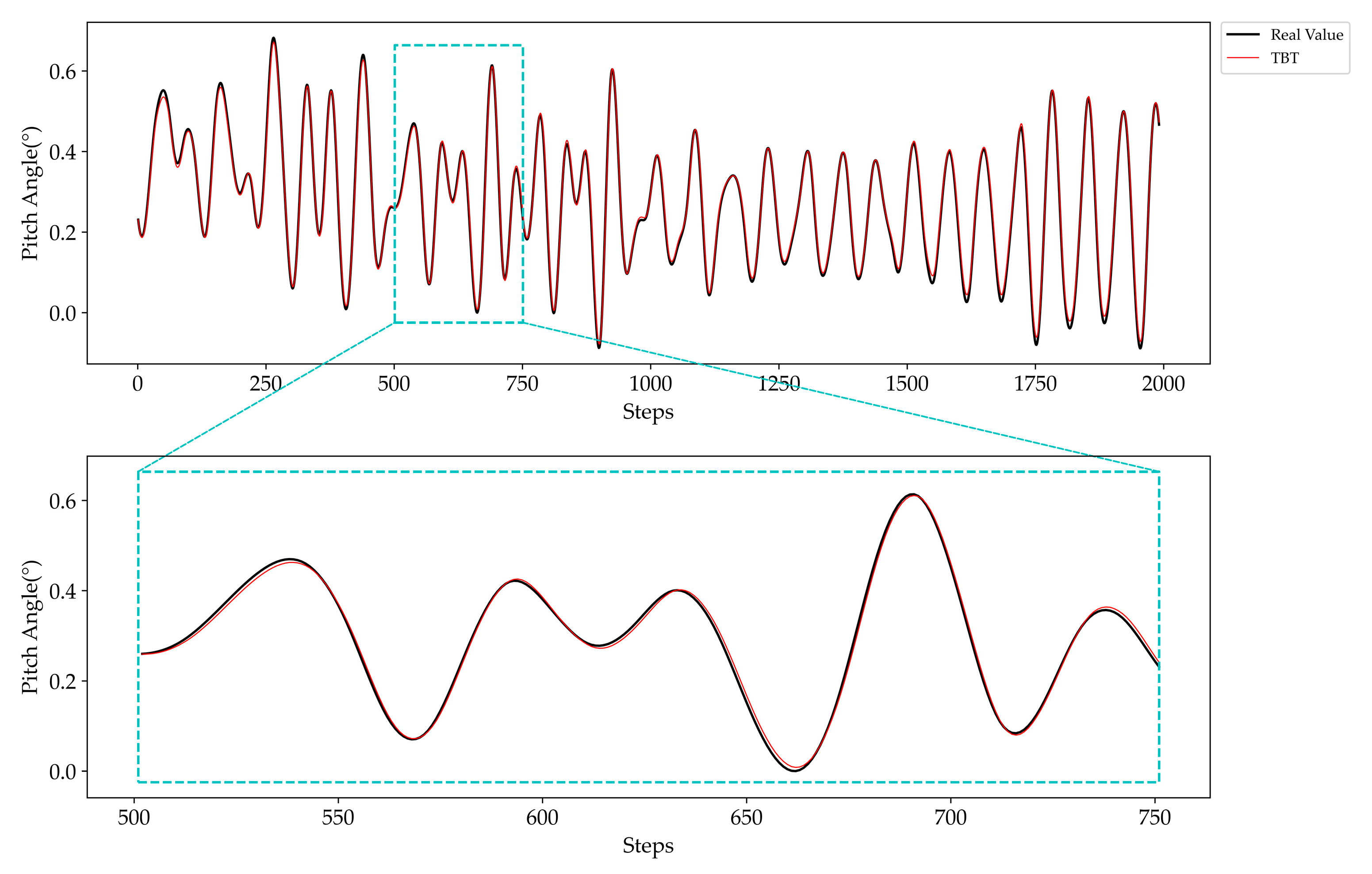
Figure 11 displays the prediction results of the USV pitch angle using the TBT hybrid model. In Figure 11, the real pitch angle is represented by a black solid line, while the red solid line represents the predicted value. In Figure 11, it is clear that the pitch angle exhibits clearer periodic characteristics and is more stable when compared with the roll angle. Therefore, predicting the pitch angle is much less challenging than predicting the roll angle. As can be seen, the TBT hybrid model can accurately capture the changing trend of the true value and closely track the true value with minimal deviation throughout the prediction process. Especially at the extreme values that are significantly related to the USV motion attitude, the prediction value rarely shows large deviations from the true value.

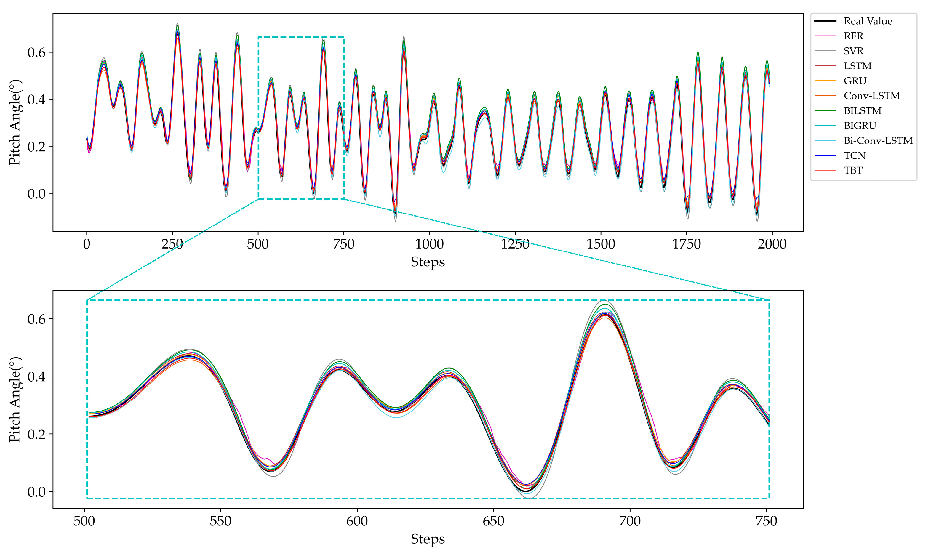
Figure 12 shows the prediction results of different models in predicting the pitch angle. As depicted in Figure 12, all models generally exhibit the ability to track the changes in the real pitch angle over time. However, during continuous changes in the true value curve, the LSTM model performs better than the GRU model; overall, the effects of the LSTM, GRU, and Conv-LSTM models exhibit similarities in pitch angle prediction tasks. The TCN model predicts well at peak points; however, there is a notable difference between the TCN model and the true value curve for trough points. The SVR model continued to struggle with accurately predicting the pitch angle under rapid changes in the ground truth value at extreme points. The performance of the RFR model is relatively better, but there is still a significant deviation between the predicted value and the real value, and the fluctuation in the real value cannot be accurately predicted. Similarly, for the pitch angle prediction, the bi-directional architectures of various RNN models did not demonstrate a superior performance at extreme points in comparison to the unidirectional counterparts.

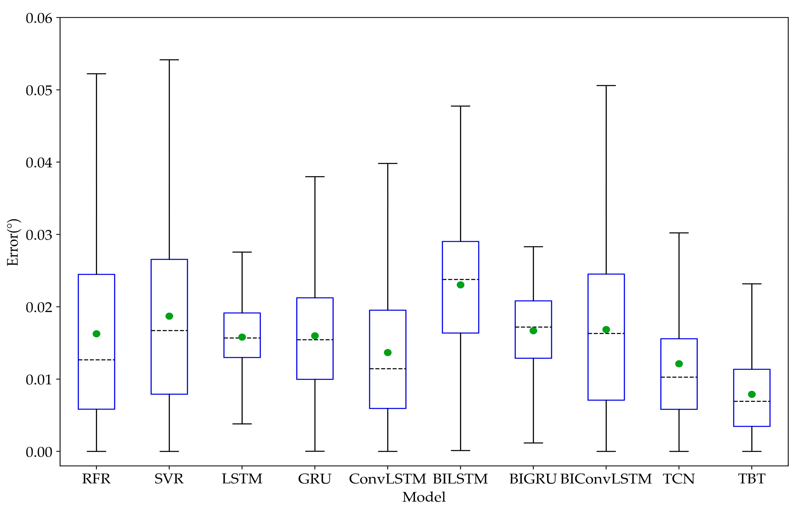
Figure 13 shows the box plot of the prediction errors of several models for the pitch angle prediction task. It can be seen that the median of the TBT hybrid model prediction error box plot is the smallest at 0.007. In contrast, the medians of the other nine error box plots are 0.013, 0.017, 0.016, 0.015, 0.011, 0.024, 0.017, 0.016, and 0.010. At the same time, the IQR of the TBT hybrid model prediction error box plot is 0.008, while the IQRs of the other nine error box plots are 0.019, 0.019, 0.006, 0.011, 0.014, 0.013, 0.008, 0.017, and 0.010. Despite the IQR of the TBT model not being the smallest, the TBT hybrid model exhibits the smallest mean and median errors, along with the minimum and maximum error values. This suggests that the dispersion of prediction errors of the TBT hybrid model is minimized, demonstrating its superior performance in terms of error distribution. In other words, the TBT hybrid model prediction error is more concentrated, with a smaller error variation range and lower prediction error. As can be seen in Figure 10, the mean value of the TBT hybrid model prediction error box plot is 0.008, while the mean values of the other models are 0.016, 0.019, 0.016, 0.016, 0.014, 0.023, 0.017, 0.017, and 0.012.

To further assess the prediction performance of different models,

Table 5. USV motion prediction evaluation index comparison of different models.

DOF	Model	MSE	MAE	MAPE	${\mathbf{R}}^2$
Roll angle (°)	RFR	0.0611	0.0771	16.56	0.9273
	SVR	0.0285	0.1114	18.96	0.9660
	LSTM	0.0096	0.0667	16.61	0.9885
	GRU	0.0092	0.0672	17.48	0.9891
	Conv-LSTM	0.0084	0.0747	20.37	0.9900
	Bi-LSTM	0.0179	0.0719	18.79	0.9787
	Bi-GRU	0.0135	0.0758	21.75	0.9839
	Bi-Conv-LSTM	0.0216	0.0898	21.27	0.9743
	TCN	0.0139	0.0876	19.66	0.9834
	TBT	0.0026	0.0441	15.97	0.9969
Pitch angle (°)	RFR	0.0004	0.0163	24.42	0.9824
	SVR	0.0005	0.0187	24.75	0.9794
	LSTM	0.0003	0.0158	24.66	0.9889
	GRU	0.0003	0.0159	28.29	0.9867
	Conv-LSTM	0.0003	0.0137	25.70	0.9884
	Bi-LSTM	0.0006	0.0230	21.85	0.9749
	Bi-GRU	0.0003	0.0167	19.19	0.9875
	Bi-Conv-LSTM	0.0004	0.0169	18.62	0.9834
	TCN	0.0002	0.0121	24.92	0.9905
	TBT	0.0001	0.0079	12.52	0.9962

The numbers in bold in the table represent the maximum and minimum values of the metrics.

displays different evaluation metrics, including the MSE, MAE, MAPE, and ${\mathrm{R}}^2$.

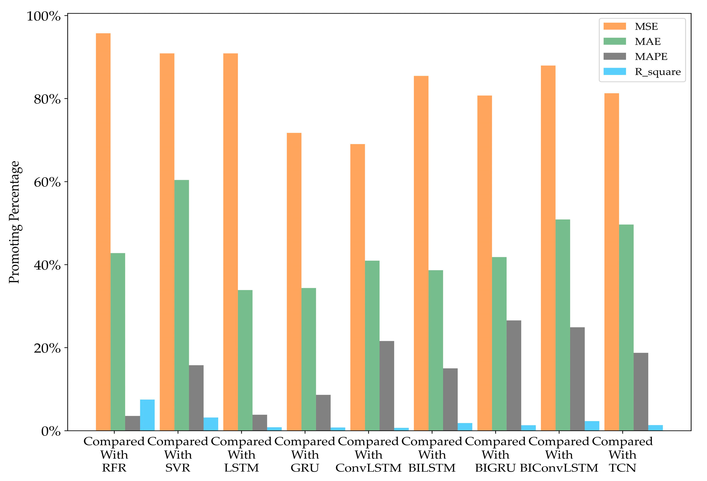
Additionally,

Table 6. Prediction promotion percentage comparison of different models.

DOF	Model	PMSE	PMAE	PMAPE	$\mathbf{P}{\mathbf{R}}^2$
Roll angle (°)	RFR	95.74%	42.80%	3.56%	7.51%
	SVR	90.88%	60.41%	15.77%	3.2%
	LSTM	72.92%	33.88%	3.85%	0.85%
	GRU	71.74%	34.37%	8.64%	0.79%
	Conv-LSTM	69.05%	40.96%	21.6%	0.70%
	Bi-LSTM	85.47%	38.66%	15.01%	1.86%
	Bi-GRU	80.74%	41.82%	26.57%	1.32%
	Bi-Conv-LSTM	87.96%	50.89%	24.92%	2.32%
	TCN	81.29%	49.66%	18.77%	1.37%
Pitch angle (°)	RFR	75.0%	51.53%	48.73%	1.40%
	SVR	80.00%	57.75%	49.41%	1.72%
	LSTM	66.67%	50.00%	49.23%	0.74%
	GRU	66.67%	50.31%	55.74%	0.96%
	Conv-LSTM	66.67%	42.34%	51.28%	0.79%
	Bi-LSTM	83.33%	65.65%	42.70%	2.18%
	Bi-GRU	66.67%	52.69%	34.76%	0.88%
	Bi-Conv-LSTM	75.00%	53.25%	32.76%	1.30%
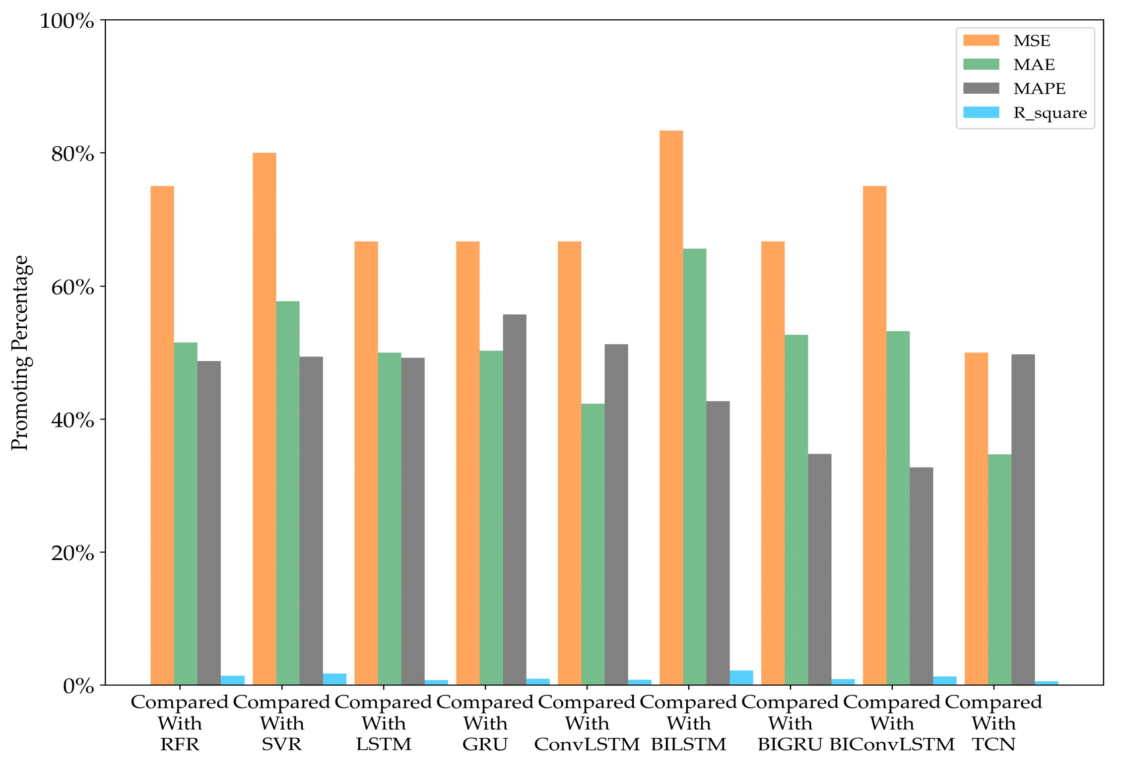
	TCN	50.00%	34.71%	49.76%	0.58%

illustrates the promotion percentage of the TBT hybrid model in comparison to other models across different evaluation metrics.

Table 5 and Table 6 present the results of the evaluation indices, indicating that the TBT model outperforms other models in both roll angle and pitch angle prediction tasks. The proposed TBT hybrid model demonstrates significant advantages across all four evaluation indicators, showcasing improvements of at least 66.67%, 33.88%, 3.56%, and 0.58% compared to the other nine models on two different tasks. These substantial improvements can be attributed to its capability to simultaneously capture spatial and temporal features dynamically.

Based on the aforementioned analysis, the TBT hybrid model can effectively capture the time-series characteristics and spatial relationship of USV motion data, and accurately fits real data. Through the analysis of the experiment, it can be seen that the TBT hybrid model proposed in this study successfully captures the transformation of real motion data. The prediction effect is more accurate, stable, and dependable compared to the other models, thereby providing a solid foundation for a further analysis of its safe navigation capabilities.

4.5. Ablation Experiments

The purpose of this section is to compare the performance of different variants of the proposed model; concretely, the ablation experiments were performed to verify the contributions of the Conv-1D, TPA, and TCN-Bi-LSTM residual models to the improved outcomes of the TBT model. These experiments were conducted on the same datasets and environment, including the training and testing of different model variants. Table 6 and

Table 7. The results of the ablation experiments.

DOF	Model	MSE	MAE	MAPE	${\mathbf{R}}^2$
Roll angle (°)	A1	0.0326	0.0710	16.41	0.9612
	A2	0.0129	0.0579	17.99	0.9847
	A3	0.0200	0.0721	18.10	0.9762
	A4	0.0179	0.0719	18.79	0.9787
	A5	0.0026	0.0441	15.97	0.9969
Pitch angle (°)	A1	0.0004	0.0166	16.54	0.9836
	A2	0.0004	0.0150	17.66	0.9858
	A3	0.0005	0.0180	18.90	0.9810
	A4	0.0006	0.0230	21.85	0.9749
	A5	0.0001	0.0079	12.52	0.9962

represent the results of the ablation experiments. The ablation experiments involve the following variations:

• A1: TBT model without the Conv-1D feature extractor at the end. Use fully connected layer to directly output predicted values.
• A2: TBT model without the TPA mechanism. Pass the output of the preorder components directly to Conv-1D feature extractor and fully connected layer to obtain predicted values.
• A3: TBT model without the TPA mechanism and Conv-1D feature extractor simultaneously. Only the basic TCN-Bi-LSTM residual structure is retained to obtain predicted values.
• A4: TBT model without the TPA mechanism, Conv-1D feature extractor, or TCN module simultaneously (i.e., the Bi-LSTM model).
• A5: The whole TBT model proposed in this paper.

In the ablation experiments, the parameters of each variant model were kept consistent with the full TBT model, the preprocessed multivariate USV motion data were input into several models separately, and the values of MSE, MAE, MAPE, ${\mathrm{R}}^2$, and the corresponding promoting percentage are reported in Table 7 and

Table 8. The promoting percentage of the ablation experiments.

DOF	Model	PMSE	PMAE	PMAPE	${\mathbf{P}\mathbf{R}}^2$
Roll angle (°)	A1	92.02%	37.89%	2.68%	3.71%
	A2	79.84%	23.83%	11.23%	1.24%
	A3	87.00%	38.83%	11.77%	2.12%
	A4	85.47%	38.66%	15.01%	1.86%
Pitch angle (°)	A1	75.00%	52.41%	24.30%	1.28%
	A2	75.00%	47.33%	29.11%	1.05%
	A3	80.00%	56.11%	33.76%	1.55%
	A4	83.33%	65.65%	42.70%	2.18%

.

As shown in Table 7 and Table 8, compared with the prediction results of the Bi-LSTM model (i.e., A4), the prediction accuracy of the TCN-Bi-LSTM residual model (i.e., A3), which is a combination of the Bi-LSTM model and the TCN, is significantly improved, with the roll angle and pitch angle prediction results obtaining an improvement of 3.67% and 13.50% in the key evaluation index, MAPE, respectively. Such an improvement can be attributed to the incorporation of the TCN as well as the introduction of the residual structure; the ability of the model to capture temporal features is improved accordingly. However, the model is still unable to carry out joint spatial-temporal feature extraction for the multiple coupled USV motion data input into the model, so the improvement in the prediction accuracy is very limited.

To further explore the effects of the Conv-1D model on the model’s performance, in A1, the model replaces the back-end Conv-1D layer with a fully connected layer; from the experimental results, the model’s performance of removing Conv-1D shows a certain degree of degradation, and compared with the complete TBT model, there are decreases in the key evaluation index, MAPE, by 2.76% and 32.11%. In addition, the other evaluation metrics of A1 are also slightly worse than the other cases, which may be caused by the fact that the removal of the local feature extraction capability of Conv-1D leads to a certain degree of decline in the model’s ability to finely perceive the trend of data changes, which will affect the model’s prediction accuracy near the extreme values, and thus manifests itself in evaluation metrics, such as the MSE, resulting in the value of these metrics to be substantially reduced.

In A2, the hidden states derived from the front component of the model are propagated through subsequent Conv-1D and fully connected layers, resulting in the computation of the final output. Based on the experimental findings, it is evident that the omission of the TPA mechanism has a more pronounced impact on the model compared to the exclusion of Conv-1D concerning the key evaluation metric, MAPE. This leads to the conclusion that the TPA mechanism plays a more crucial role in enhancing the prediction accuracy of the model as opposed to Conv-1D. One possible explanation for this observation is attributed to the TPA mechanism’s ability to capture spatial correlations present in the data. Furthermore, its adaptive allocation of different weights to individual input features contributes to reinforcing the model’s ability to characterize relationships among distinct variables, thereby further improving the accuracy of predictions.

5. Discussion

To address the problem of insufficient accuracy of multivariate predictions caused by the limitations of traditional and single prediction models in effectively capturing hidden multidimensional information, this paper proposes a multivariate USV motion data method based on the TCN-Bi-LSTM-TPA model. Compared with other models in experiments, the effectiveness of the proposed model is verified.

The experiments conducted in this study can be divided into two aspects. Firstly, a comprehensive comparison of the model’s performance is carried out using datasets, including roll and pitch angles. Secondly, the effectiveness of the different components of the model is explored through ablation experiments.

For the roll angle prediction task, the roll angle data show an irregular trend and an obvious non-stationarity, making the prediction more difficult. The proposed TBT model maintains high prediction accuracy, even when the roll angle varies drastically, thanks to the contribution of the TPA mechanism and Conv-1D at the end of the model, which extract spatial correlations. This can be seen from the discussion of ablation experiments. The prediction results of the LSTM and GRU models are similar, and neither of them can predict accurately at the peak of the true value curve. However, none of the models can make accurate predictions at the extreme points of the true value curve, as seen from the MSE values in Table 5. The MSE is particularly sensitive to data changes, providing insights into the model’s predictive performance during data peaks, where the changes are most intense. Therefore, to some extent, the MSE can reflect the predictive performance of the model at the peaks. The Conv-LSTM model applies convolutional operations in conjunction with LSTM, allowing for the extraction of features from input data through convolutions before conducting sequence feature extractions. This operation significantly aids the model in effectively capturing intricate spatiotemporal features inherent in the input data, resulting in a better MSE score compared to that of the LSTM and GRU models. For the bi-directional structure models of several RNN models, it can be seen in Table 5 that the bi-directional structure models perform worse than the unidirectional structure models for several evaluation metrics.

For the pitch angle prediction, the trend of the pitch angle is more regular, which means it is easier to predict. By studying the predictions of both the roll angle and pitch angle, the prediction performance of the TBT hybrid model can be comprehensively demonstrated for targets with different statistical features. As illustrated in Figure 13, the TBT hybrid model has the smallest median and mean prediction errors, and the smallest IQR among the ten models is the LSTM model, which indicates that its prediction errors are the most concentrated. However, with the combined median and mean prediction errors, the TBT hybrid model still has the best performance. As with the cross-tilt prediction, for several deep learning models, the prediction results of the LSTM, GRU, and Conv-LSTM models do not show significant differences, and the Conv-LSTM model does not outperform the other two models at the extremes, which may be due to the experimentally selected pitch angle datum being smoother and having a more pronounced pattern than the troll angle datum. Therefore, the LSTM model may not present the best performance. This may be due to the fact that the experimentally selected pitch angle data are smoother and have a more pronounced pattern than the roll angle data, and thus the prediction performance of the LSTM and GRU models at the extreme points does not lag behind that of the Conv-LSTM model too much. From Table 7, it can be seen that the bi-directional structural models outperform the unidirectional structural models for pitch angle prediction in contrast to the roll angle prediction. This may depend on the pattern of the input, as models with a bi-directional structure rely more on contextual information, which may be more effective for data with broadly similar trends of change.

The bar charts in Figure 14 and Figure 15 show the promoting percentages in the prediction accuracy of the TBT hybrid model compared to the other nine models on the four evaluation metrics. It is apparent that the results of the proposed TBT model have improved compared to the other nine models; improvements in the overall accuracy are consistently concentrated between 0.5% and 96%. Meanwhile, the trends of the four indicators for the two prediction tasks are basically the same, verifying the validity of the TBT model, and, at the same time, the specific advantages and disadvantages of each comparative model are more intuitively represented.

6. Conclusions

USV motion prediction can provide important information for a USV’s attitude control and safety navigation. A multivariate USV motion prediction method based on a TCN-Bi-LSTM-TPA (TBT) hybrid model was proposed in this study, which aimed to effectively capture hidden multidimensional information from multivariate USV motion data in both temporal and spatial aspects. The main work and conclusions of this paper are summarized as follows:

• Based on the TBT hybrid model, two motion attitudes that have a significant impact on USV status, roll angle, and pitch angle are predicted. Multivariate USV motion data, including roll angle, pitch angle, relative wind speed, relative wind direction, velocity in surge, velocity in sway, and rotation rate, are normalized and inputted into the model separately. The TBT hybrid model utilizes the TCN and Bi-LSTM models to construct a residual model to extract both the short-term and long-term temporal dependencies of USV motion data. Simultaneously, the TPA module is employed to capture spatial features from the multivariate input. Additionally, a Conv-1D layer is incorporated to further extract local spatial features and enhance the model’s learning capability.
• To evaluate the prediction performance of the proposed model, real USV motion data are used, and a comparison is made with several classic and advanced motion prediction models, including RFR, SVR, LSTM, GRU, Conv-LSTM, Bi-LSTM, Bi-GRU, Bi-Conv-LSTM, and TCN. Eight evaluation metrics are utilized to measure the performances of all the prediction models. The experimental results indicate that the TBT model exhibits superior prediction accuracy, with an MSE, MAE, MAPE, and ${\mathrm{R}}^2$ of 0.0026, 0.0441, 15.97%, and 0.9969 for the roll angle prediction, and 0.0001, 0.0079, 12.52, and 0.9969 for the pitch angle prediction, respectively.
• To verify the effectiveness of the proposed model, ablation experiments are conducted. The results show that adding a TPA mechanism and Conv-1D layer helps improve the multivariable prediction performance of the model. This study provides a new solution for multivariate USV motion prediction.

Considering the extremely short sampling frequency of USV sensors when collecting motion data, the time available for the USV to make attitude adjustments based on the prediction results is also limited. Therefore, future research should focus on expanding the prediction time range while maintaining the prediction accuracy in order to provide a sufficient response time for USV control based on prediction feedback.