Numerical Study on the Swimming and Energy Self-Sufficiency of Multi-Joint Robotic Fish

Abstract

Energy is one of the primary challenges in the long-term operation of robotic fish. The research on combining wave energy-harvesting technology with robotic fish for energy supplementation is not extensive, and there is insufficient comprehensive analysis on energy harvesting from waves and energy costs during swimming. Therefore, the energy self-sufficiency of multi-joint robotic fish is investigated by employing the coupling method of smoothed particle hydrodynamics (SPH) and multi-body dynamics in this study. A reversible energy conversion mechanism is applied to the robotic fish, serving as a driving system during swimming and as a power take-off (PTO) system during energy harvesting. The energy costs of the multi-joint robotic fish under various undulation parameters (including amplitude, frequency, and body wavelength) are analyzed, along with an examination of the influence of the PTO system on energy harvesting. The results show that, compared to the undulation amplitude and body wavelength, the undulation frequency has the greatest impact on swimming efficiency and energy costs, with low-frequency swimming being advantageous for efficient energy utilization. Additionally, the damping coefficient of the PTO system directly affects energy-harvesting efficiency, with higher energy-harvesting power achievable with an optimal PTO system parameter. Through a comprehensive analysis of energy costs and energy harvesting, it is concluded that the achievement of energy self-sufficiency for multi-joint robotic fish in marine environments is highly feasible.

1. Introduction

After billions of years of evolution in nature, fish surpass the capabilities of current underwater vehicles. The swimming modes of fish are classified into the body and/or caudal fin (BCF) and median and/or paired fin (MPF) modes [1] based on the generation of thrust by different body parts. Among these, the eel-like (anguilliform) locomotion mode, a type of BCF propulsion mode, is known for its minimal energy costs per unit distance [2] and high stability during swimming, attracting significant attention from researchers in recent years.

In the past few decades, extensive efforts have been made to understand the physical mechanisms, modeling, and motion control of eel-like fish. Gillis [3] and Gray [4] employed video recordings to capture the locomotion of eels, deriving the kinematic parameters of undulatory motion through the analysis of their body movements. Fish et al. [5], Muller et al. [6], and Triantafyllow et al. [7] utilized experimental flow visualization techniques to reveal the wake structure and explain how the vortices contribute to enhanced propulsion efficiency. Minami et al. [8] employed a chaos model to predict the motion trajectory of fish. Carling et al. [9] established a set of body equations based on dimensionless parameters to describe the undulatory swimming of eels and model the body outline. Additionally, they simulated the kinematics and dynamics of eel movement through the computational fluid dynamics (CFD) method, emphasizing the significant impact of viscous forces in the generation and dissipation of vortex structures around living organisms.

Meanwhile, the theoretical understanding of eel-like robotic locomotion is gradually maturing. Taylor [10] and Lighthill [11] proposed the resistive force theory and large-amplitude elongated-body theory, respectively, to calculate the fluid forces acting on the body during ideal undulatory swimming. These theories have been widely applied in the hydrodynamic modeling of robotic fish. However, due to the complexity of fluid dynamics and biological locomotion, these theoretical models typically have limited applicability. McIsaac et al. [12] proposed a dynamic model for an eel-like locomotion robot based on differential geometry tools, but this method neglects inertial forces. Boyer et al. [13] proposed a kinematic model for the continuous three-dimensional swimming of eel-like robotic fish based on the geometrically exact beam theory and Newton–Euler theory. Currently, fluid moments are often overlooked in many swimming robot models. Although some studies suggest that the influence of fluid moments on the overall motion of the system can be considered negligible, their significance cannot be disregarded in terms of the energy costs of mechanical motion [14]. Wiens et al. [15] and Khalil et al. [16] modeled fluid moments, but their algorithms involved the numerical integration of the drag and moment at each sampling interval, resulting in a lack of closed-form solutions. Candelier et al. [17] proposed a model for the reactive forces and moments acting on slender bodies, but they did not consider viscous effects. Kelasidi et al. [18] modeled the fluid forces and moments using an analytical method, yielding closed-form solutions. However, due to the highly complex and nonlinear hydrodynamics resulting from rigid body motion, their study also employed some simplified analytical forms.

With the advancement and deepening of research on biomimetic robotic fish, both theoretical and experimental studies in this field are being developed. However, underwater robotic fish are commonly situated far from traditional power sources, relying mainly on conventional options such as chemical energy batteries for their energy supplies. Currently, the capacity of batteries is limited, and they are unable to meet the energy demands for the long-term autonomy of robots [19]. The acquisition and efficient utilization of energy have emerged as crucial technological challenges that hinder their development and application. Abundant renewable energy sources such as wave energy, tidal energy, ocean currents, and thermal gradients exist in the environments in which biomimetic robotic fish operate [20]. Among them, wave energy stands out as one of the most concentrated renewable energy sources [21]. The global annual wave energy resource is estimated to amount to approximately 32,000 TWh, surpassing the global electricity consumption of 24,000 TWh in 2015 [22]. Furthermore, wave energy boasts a significantly higher energy density compared to other renewable sources, such as wind energy, being 4 to 30 times greater [23]. Accurate wave simulation is essential for studying wave energy conversion. It is imperative to meticulously capture the gas–liquid interface [24,25] when modeling waves using two-phase flow methods. In contrast, the SPH method eliminates the need for modeling the air phase, thus conferring notable advantages in tackling free surface problems, including wave propagation [26] and the interaction between rigid bodies and water [27].

The first patent for a wave energy conversion device was filed by Girard and his son in France in 1799 [28]. The number of related wave energy conversion patents had exceeded 1000 by 1980 and steadily increased thereafter [29]. Currently, wave energy conversion devices are primarily classified into oscillating water columns, oscillating bodies, and overtopping devices based on their working positions, principles, and sizes. Among these, attenuator devices are a type of oscillating body, consisting of multiple rafts connected by hinges and a PTO system at the hinges. The adjacent rafts rotate in the waves, driving the generator within the PTO system at the hinges to produce electricity. Christopher Cockrell first proposed this structure in the 1870s and developed a wave energy conversion device named the Cockrell [30]. Based on this, Ocean Power Delivery developed a wave energy conversion device named Pelamis in 2006 and deployed three Pelamis devices on the northern coast of Portugal in the latter half of 2008 [31].

Currently, most wave-energy-harvesting devices are large-scale and considered large-scale networked power supply systems. In contrast, research on integrating small-scale wave energy-harvesting devices with biomimetic robotic fish is relatively limited. Research in this field has been primarily conducted by Dong et al. [32] and Zhu et al. [33]. Dong et al. [32] proposed a method for converting wave energy into electrical power for robotic fish by using wave energy conversion devices and designed the corresponding electromechanical model for the energy-harvesting system. However, their research solely focused on energy harvesting for robotic fish, yielding experimental results that indicated low energy-harvesting efficiency. Additionally, they did not explore the relationship between power harvesting and the motor moments at the joint. Zhu et al. [33] introduced a scheme for the harnessing of wave energy using a reversible energy conversion mechanism. They conducted experimental and simulation studies on the motion characteristics of the three links under waves but did not provide a comprehensive analysis of the energy harvesting and swimming for the same body.

Considering that many studies either focus on modeling the locomotion of robotic fish or investigate wave energy harvesting of multi-joint floaters, it remains unclear whether the energy harvested from waves by robotic fish of the same shape is sufficient to meet their energy costs during swimming. Furthermore, there is a need for systematic research on how to adjust wave parameters and PTO systems to achieve efficient swimming and energy harvesting. The feasibility of robotic fish achieving energy self-sufficiency by harnessing wave energy in the ocean has not been fully evaluated. Therefore, the fluid–structure interaction (FSI) method is employed to simulate the self-propelled swimming and energy harvesting of multi-joint robotic fish in this study. The analysis focuses on the relationships between undulation parameters and swimming performance (including forward velocity, energy cost, and swimming efficiency) of multi-joint robotic fish in different swimming modes. Subsequently, the influence of the PTO system on the energy-harvesting power of the multi-joint robotic fish is discussed, and the motion characteristics are analyzed. Finally, the energy self-sufficiency of the multi-joint robotic fish is evaluated by considering both the swimming efficiency and the energy-harvesting efficiency.

The structure of this paper is as follows. Section 2 introduces the model and methodology of the numerical simulations and validates the accuracy of the numerical methods. Section 3 describes the simulation domain of the swimming and energy harvesting modes and the validation of the particle resolution. Section 4 discusses the swimming, energy harvesting, and energy self-sufficiency of the robotic fish. Conclusions are given in Section 5.

2. Methodology and Validation

The swimming and energy harvesting of multi-joint robotic fish is a problem with moving boundaries and multi-body dynamics. The coupling method of DualSPHysics and Project Chrono provides a convenient solution to this issue. DualSPHysics is a meshless solver based on the SPH method. It is coupled with Project Chrono to address the mechanical constraints between rigid bodies and interactions between multi-bodies and fluids. This coupling method is utilized for the modeling of multi-joint robotic fish.

2.1. SPH Fundamental

The SPH method discretizes a continuous field using a set of computational nodes or particles, where the physical quantities (position, velocity, density, and pressure) are approximated by interpolation of neighboring particle values. Any function $F(\mathit{r})$ can be computed using integral interpolation:

$$F(\mathit{r})=\int F({\mathit{r}}^{\prime })W(\mathit{r}-{\mathit{r}}^{\prime },h)d{\mathit{r}}^{\prime }$$

(1)

where $\mathit{r}$ is the position of the target point, and ${\mathit{r}}^{\prime }$ is the position of another point (or particle) around the target point. In discrete form, the function $F\left(\mathit{r}\right)$ is approximated by interpolating the contributions of the particles within the compact support of the kernel function as follows:

$$F\left({\mathit{r}}_a\right)\approx {\sum }_b F\left({\mathit{r}}_b\right)W\left({\mathit{r}}_a-{\mathit{r}}_b,h\right)\frac{m_b}{{\rho }_b}$$

(2)

where a is the target particle, b is a neighboring particle, m is the mass, ρ is the density, and h is the smoothing length. The weighting function W (r, h) used in this work is the Quintic Wendland kernel, defined by:

$$W\left(q\right)={\alpha }_{\mathrm{D}}{\left(1-\frac{q}{2}\right)}^4\left(2q+1\right),0\le q\le 2$$

(3)

where ${\alpha }_{\mathrm{D}}$ is a real number that ensures the kernel normalization property, q = r/h is the non-dimensional distance between particles, and r is the distance between particles a and b.

2.2. Governing Equations

DualSPHysics is based on the weakly compressible SPH (WCSPH) method, where the fluid particles are governed by the Navier–Stokes equations. The Lagrangian form of the momentum and continuity equations can be expressed as follows [34]:

$$\frac{\mathrm{d}\mathit{v}}{\mathrm{d}t}=-\frac{1}{\rho }\nabla p+\mathit{g}+\mathit{\Gamma }$$

(4)

$$\frac{\mathrm{d}\rho }{\mathrm{d}t}=-\rho \nabla \cdot \mathit{v}$$

(5)

where $\mathit{v}$ is the velocity, $t$ is the time, $p$ is the pressure, $\mathit{g}$ is the gravity, and $\mathit{\Gamma }$ is the viscosity term.

The Equation (4) can be written in SPH formalism as follows [35]:

$$\frac{d{\mathit{v}}_a}{dt}=-{\sum }_b{m}_b\left(\frac{p_b+p_a}{{\rho }_b{\rho }_a}\right){\mathbf{\nabla }}_a{W}_{ab}+\mathit{g}+{\mathit{\Gamma }}_{\mathit{a}}$$

(6)

where $m$ is the mass, and $W_{ab}$ is the Quintic Wendland kernel function.

The viscosity considered in this study is the laminar flow viscosity with a sub-particle scale model (SPS), which is stated as follows:

$${\mathit{\Gamma }}_a={\sum }_b m_b\frac{4{\upsilon }_0{\mathit{r}}_{ab}\cdot {\mathbf{\nabla }}_a{W}_{ab}}{\left({\rho }_a+{\rho }_b\right)\left(r_{ab}^2+0.01h^2\right)}{\mathit{v}}_{ab}+{\sum }_b m_b\left(\frac{{\tau }_a^{ij}+{\tau }_b^{ij}}{{\rho }_b{\rho }_a}\right){\mathbf{\nabla }}^i{W}_{ab}$$

(7)

where the first term on the right is the laminar viscosity [36], the second term is the SPS model [26], ${\upsilon }_0$ is the kinematic viscosity of the fluid, and $\tau$ is the SPS stress tensor.

The Equation (5) can be written in the discrete SPH formalism and augmented with a density diffusion term as follows:

$$\frac{d{\rho }_a}{dt}={\sum }_b m_b{\mathit{v}}_{ab}\cdot {\mathbf{\nabla }}_a{W}_{ab}+2\delta h{c}_s{\sum }_b \left({\rho }_{ba}^T-{\rho }_{ab}^H\right)\frac{{\mathit{r}}_{ab}\cdot {\nabla }_a{W}_{ab}}{r_{ab}^2}\frac{m_b}{{\rho }_b}$$

(8)

where the second term on the right is the density diffusion term [37], δ is a parameter governing the diffusive term, $c_s$ is Smagorinsky’s constant, and subscripts T and H indicate the total and hydrostatic components of the density for a weakly compressible fluid.

In the SPH method, the fluid is considered a weakly compressible formulation. To close Equations (6) and (8), an equation of state is employed to obtain the fluid pressure (p) from the particle density, which is stated as follows:

$$p=\frac{c_s^2{\rho }_0}{\gamma }\left[{\left(\frac{\rho }{{\rho }_0}\right)}^{\gamma }-1\right]$$

(9)

where ${\rho }_0$ is the reference density of the fluid, and $\gamma$ is the polytropic constant.

2.3. Project Chrono and Coupling with DualSPHysics

Project Chrono is an open-source library for multiphysics simulations, enabling the numerical modeling of mechanical constraints and collisions between objects [38]. It can simulate the behavior of objects of arbitrary shapes in a fluid via coupling with DualSPHysics. The solver can integrate the effects of kinematic-type constraints as well as dynamic-type constraints and internal collisions [39]. Additionally, it can simulate externally applied forces and moments and motion trajectories with arbitrary degrees of freedom [40]. In this study, both the connection between the links and the PTO system of energy harvesting require coupling between DualSPHysics and Project Chrono.

The complete multi-body model is provided through the coupling of DualSPHysics and Project Chrono [41] as follows:

$$\frac{d\mathit{q}}{dt}=\mathit{L}\left(\mathit{q}\right)\mathit{v}$$

(10)

$$\mathit{M}\frac{d\mathit{v}}{dt}={\mathit{f}}_t\left(t,\mathit{q},\mathit{v}\right)$$

(11)

$${\mathit{f}}_t\left(t,\mathit{q},\mathit{v}\right)={\mathit{f}}_e-{\mathit{f}}_c$$

(12)

where $\mathit{q}$ is the generalized position, $\mathit{L}\left(\mathit{q}\right)$ is the linear transformation, v is the velocity, M is the mass matrix, ${\mathit{f}}_t$ is the total force, ${\mathit{f}}_e={\mathit{f}}_e\left(t,\mathit{q},\mathit{v}\right)$ is the external force, and ${\mathit{f}}_c={\mathit{f}}_c\left(\mathit{q},t\right)$ is the constraint force.

The constraints for mechanical joints on links are defined as follows:

$${\mathit{f}}_c=\alpha \mathit{\theta }+\beta \dot{\mathit{\theta }}$$

(13)

where $\mathit{\theta }$ is the angle of rotation, $\dot{\mathit{\theta }}$ is the angular velocity, and $\alpha$ and $\beta$ are the rotational stiffness and damping coefficient, respectively.

The process of coupling to compute the displacement and velocity of rigid bodies under mechanical constraints using DualSPHysics and Project Chrono can be segmented into three continuous phases: (1) the computation of forces on the rigid body, (2) the multi-body dynamics solution, and (3) the updating of particle attributes. The comprehensive details and validation of the coupling can be found in [42].

2.4. Model and Evaluation of Multi-Articular Robotic Fish

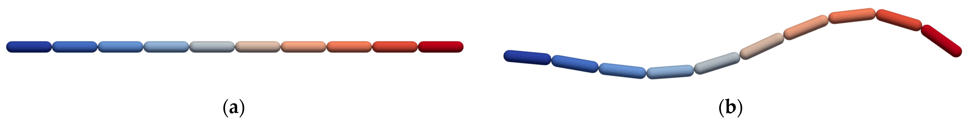
2.4.1. The Model of Eel-like Locomotion

The main characteristic of eel-like locomotion is the gradual increase in body undulation amplitude from the head to the tail, which induces forward swimming through a periodic backward-traveling wave. The lateral displacement ($y_s(s,t)$) of the body midline is given by the following (Carling et al. [9]; Kern et al. [43]):

$$y_s\left(s,t\right)=a{L}_c\frac{s/L_c+0.03125}{1.03125}\sin \left[\phi \left(s/L_c-tf\right)\right]$$

(14)

where $L_c$ is the total length of the midline, $a$ is the amplitude coefficient, $s$ is the arc length along the body midline, f is the undulation frequency, and $\phi$ is the phase controlling the body wavelength.

Equation (14) needs to be discretized to control the motion of the robotic fish. Consider a robotic fish with N links arranged along its midline, where the number of joints is N − 1. Therefore, the midline of the robotic fish consists of N straight segments. The positions of the N − 1 joints are given by the following:

$$s_i=\frac{i{l}_c}{L_c}=\frac{i}{N}$$

(15)

where $i=1,\cdots ,N-1$ is the number of joints, and $l_c=L_c/N$ is the length of each link. Consequently, the motion equation at each joint is as follows:

$$y_s\left(i,t\right)=a{L}_c\frac{i/N+0.03125}{1.03125}\sin \left[\phi \left(\frac{i}{N}-tf\right)\right]$$

(16)

Figure 1 illustrates the joint displacement and the angles of the links of the multi-joint robotic fish, demonstrating the conversion between joint displacement and link rotation angles. The angle ${\theta }_i$ for the link is given by the following [44]:

$${\theta }_i=\mathrm{a}\mathrm{r}\mathrm{c}\mathrm{s}\mathrm{i}\mathrm{n}\left(\frac{y_s\left(i,t\right)-y\left(i-1,t\right)}{l_c}\right) i=1,\cdots ,N$$

(17)

2.4.2. Energy Costs and Efficiency of Swimming

The forward thrust of a multi-joint robotic fish is generated by the interaction between its body and the surrounding fluid. Consequently, the total energy input to the links is divided into two components: the kinetic energy associated with the body motion of the fish and the energy dissipated into the surrounding fluid. Assuming negligible frictional losses within the links of the multi-joint robotic fish, the total energy input to the system (E_total) is equal to the sum of the kinetic energy (E_kinetic) and the energy dissipated into the surrounding fluid (E_fluid) [45]:

$$E_{total}=E_{kinetic}+E_{fluid}$$

(18)

The total energy (E_total) input into the system per cycle is as follows:

$$E_{total}={\int }_t^{t+T_c}\left(\sum _{i=1}^{N-1} T_i\left(t\right){\dot{\varphi }}_i\left(t\right)\right) dt$$

(19)

where T_c is the period of swimming, $T_i$ is the input moment, and $\dot{{\varphi }_i}$ is the angular velocity difference of adjacent links, defined as ${\dot{\varphi }}_i={\dot{\theta }}_{i+1}-{\dot{\theta }}_i$.

The average power of the input energy is given by the following:

$${\overline{P}}_{total}=\frac{1}{T_c}{\int }_t^{t+T_c}\left(\sum _{i=1}^{N-1}{T}_i\left(t\right){\dot{\varphi }}_i\left(t\right)\right)dt$$

(20)

It is crucial to select optimal locomotion modes in order to minimize energy costs for multi-joint robotic fish. The dimensionless swimming efficiency is employed to assess the effectiveness of the multi-joint robotic fish in converting the input energy into forward motion [43].

$${\eta }_m=\frac{{\overline{P}}_{forwardmotion}}{{\overline{P}}_{total}}$$

(21)

$${\overline{P}}_{forwardmotion}=\frac{1}{T_c}{\int }_t^{t+T_c}\left(\sum _{i=1}^N \frac{1}{2}{m}_i{u}_i^2\right) dt$$

(22)

$${\overline{P}}_{motion}=\frac{1}{T_c}{\int }_t^{t+T_c}\left(\sum _{i=1}^N \frac{1}{2}{m}_i\left(u_i^2+v_i^2\right)+J_i{\dot{\theta }}_i^2\right) dt$$

(23)

where η_m is the swimming efficiency, ${\overline{P}}_{forwardmotion}$ is the average forward kinetic energy, $m_i$ is the mass, $u_i$ is the forward velocity, ${\overline{P}}_{motion}$ is the average kinetic energy, $J_i$ is the moment of inertia, and $v_i$ is the lateral velocity.

2.4.3. PTO System for the Energy-Harvesting Model

The relative rotation of the adjacent links in waves drives the motor at the joints to generate electricity. The influence of the motor on the link manifests as a resistance moment. Consequently, the resistance of the motor system is simplified to a resistance moment that is directly proportional to the relative rotation angle and angular velocity of the adjacent links [46]:

$$M_{i(i+1)}=\alpha {\varphi }_i+\beta \dot{{\varphi }_i}$$

(24)

where $M_{i(i+1)}$ is the resisting moment between links i and i + 1, and ${\varphi }_i$ is the rotation angle difference between adjacent links, defined as ${\varphi }_i={\theta }_{i+1}-{\theta }_i$. The coefficients $\alpha$ and $\beta$ are related to the motor system, with $\alpha$ being set to 0 in this work [33].

2.4.4. Energy Harvesting and Efficiency

The energy ${(E}_w)$ per unit time and unit length of the second-order Stokes wave in the propagation direction is given by the following [47]:

$$E_w=\frac{1}{2}{\rho }_{w}g{A}^2\left(1+\frac{1}{8}{\left(Ak\right)}^2\left(5+\frac{68 {\sinh }^{4}kd+57 {\sinh }^{2}kd+18}{4 {\sinh }^{6}kd}\right)\right)$$

(25)

where $A$ is the wave amplitude, ${\rho }_w$ is the water density, $k=2\pi /L_s$ is the wavenumber, $L_s$ is the wavelength, and $d$ is the water depth.

The resistance moment of the adjacent links can be calculated using Equation (24), resulting in harvested energy:

$$E_s={\int }_t^{t+T_s}\left(\sum _{i=1}^{N-1}{M}_{i\left(i+1\right)}\left|{\dot{\theta }}_i-{\dot{\theta }}_{i+1}\right| \right)dt$$

(26)

$${\overline{P}}_s=\frac{1}{T_s}{\int }_t^{t+T_s}\left(\sum _{i=1}^{N-1}{M}_{i\left(i+1\right)}\left|{\dot{\theta }}_i-{\dot{\theta }}_{i+1}\right| \right)dt$$

(27)

where $E_s$ is the harvested energy, $T_s$ is the wave period, and ${\overline{P}}_s$ is the average harvested power.

The energy-harvesting efficiency is employed to evaluate the relationship between the energy harvested by the multi-joint robotic fish and the wave energy of the fluid below it:

$${\eta }_s=\frac{E_s}{T_s{L}_c{E}_w}$$

(28)

where ${\eta }_s$ is the energy-harvesting efficiency of the robotic fish, and $L_c$ is the length of the robotic fish.

2.5. Numerical Model Validation

The pitching motion of the classic NACA0012 airfoil is utilized to validate the accuracy of the swimming for multi-joint robotic fish [48]. The simulation domain has a length of 0.7 m and a width of 0.4 m, with a water density of ρ_w = 1000 kg/m³ and a dynamic viscosity of μ = 1 × 10⁻³ Pa∙s. The airfoil has a chord length of c = 0.1 m and a density of ρ_s = 1000 kg/m³, and the simulation parameters are set as follows: θ = 5°, k = 2πfc/u = 9, and Reynolds number Re = ρ_wuc/μ = 1.35 × 10⁴. Figure 2a illustrates the wake formed by two counter-rotating vortices and the phenomenon of wake vortex shedding. Additionally, the thrust coefficient (C_T = 2F_T/(ρ_wu² c)) is computed and compared with the findings of Lu et al. [48], as shown in Figure 2b. The verification demonstrates that the thrust coefficient in this study agrees well with the literature, indicating the relatively accurate simulation of the pitching motion of the airfoil. The results demonstrate that the coupling method based on DualSPHysics and Chrono is accurate and reliable, providing a foundation for further research on the motion of multi-joint robotic fish.

In order to evaluate the performance of DualSPHysics in simulating the wave-induced motions of robotic fish during wave energy harvesting, a validation case involving a floating box in waves is selected [49]. The tank has a length of 12 m and a height of 2 m, with a water depth of 0.4 m. The water density is ρ_w = 1000 kg/m³, and the dynamic viscosity is μ = 1 × 10⁻³ Pa∙s. The width and the height of the floating body are 0.3 m and 0.2 m, respectively. The floating body is homogeneous and its density is ρ_s = 500 kg/m³. The height of the wave is 0.1 m, and the period is 1.2 s. The velocity field of the floating body in waves is shown in Figure 3a. The results in this study are compared with the experimental results of Ren et al. [49], as shown in Figure 3b. It can be observed that the present result is in good agreement with experimental results, confirming the accuracy of the calculation method and enabling research on energy harvesting for multi-joint robotic fish in wave environments.

3. Simulation Domain and Resolution Verification

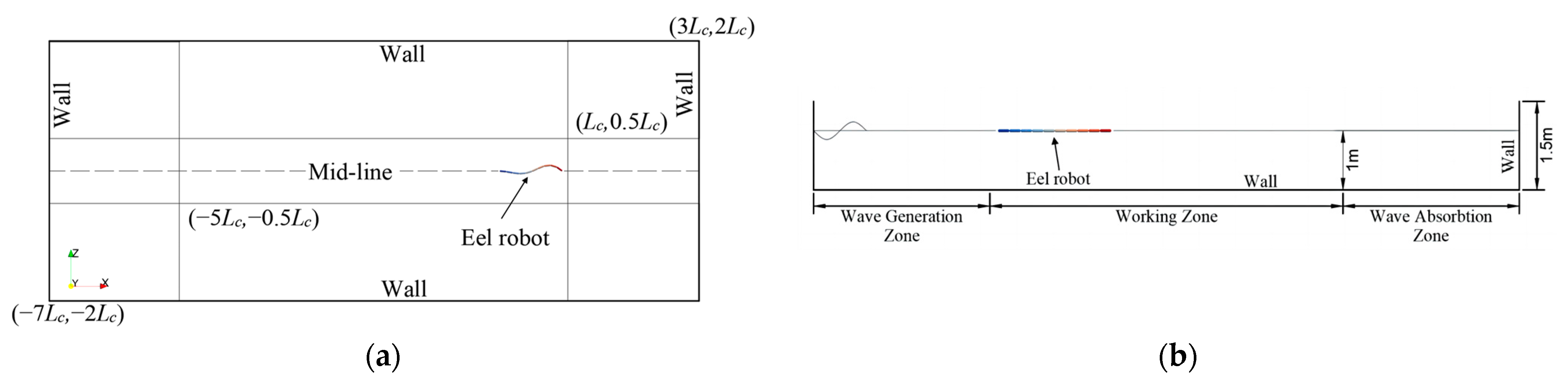
3.1. Simulation Setting

We investigate two operational states of the multi-joint robotic fish, which are the swimming state and the energy-harvesting state. In the swimming state, the robotic fish is submerged in water and actively controls the rotation of its links to generate forward motion, as shown in Figure 4a. In the energy-harvesting state, it floats on the sea surface and relies on waves to drive the rotation of its joints to generate electrical energy, as shown in Figure 4b. It is worth noting that the direction of the positive y-axis is inward and perpendicular to the XOZ plane.

The robotic fish is positioned inside a tank, as illustrated in Figure 4a. The robotic fish consists of 10 links with a total length of 2 m. Each link has a length of 0.2 m and a width of 0.05 m, with a density of ρ_s =1000 kg/m³. The simulation domain is selected as a rectangular tank with a length of 10 body lengths by 4 body lengths, giving overall dimensions of 20 m and 8 m, respectively [50]. The surrounding fluid comprises water, with a density of ρ_w =1000 kg/m³ and dynamic viscosity of μ = 1 × 10⁻³ Pa∙s. The robotic fish starts with a “C-shaped” configuration and gradually scales the amplitude of its body from zero to the distribution defined in Equation (14), as shown in Figure 5. The undulation amplitude coefficient a (amplitude as aL_c), undulation frequency f, and undulation phase φ (controlling body wavelength) of the multi-joint robotic fish are key variables that directly affect its swimming efficiency. To comprehensively consider the influence of different locomotion modes on the swimming efficiency of the robotic fish, specific parameter values are provided based on the research by Carling et al. [9] and Kern et al. [43] on the locomotion of real eels: a is set to 0.0625, 0.09375, 0.125, 0.15625, and 0.1875, respectively; f is set to 0.5 Hz, 0.75 Hz, 1.0 Hz, 1.25 Hz, and 1.5 Hz, respectively; φ is set to π, 1.5π, 2π, 2.5π, and 3π, respectively.

The schematic diagram of the energy-harvesting model of the multi-joint robotic fish is illustrated in Figure 4b. The piston-type wave maker is located at the left end of the tank. Numerical lateral damping zones are implemented on the right side of the tank to absorb and nullify reflections from the right wall, minimizing their impacts on the wave field. The robotic fish adjusts its density by discharging water to float on the surface of the water. The links of the robotic fish undergo relative rotation influenced by the waves, achieving energy harvesting from the waves. The numerical wave tank has a length of 12 m, and it is divided into three distinct zones: the wave generation zone, extending from 0 to 3 m; the working zone, spanning 3 to 9 m; and the lateral damping zone, covering the final 9 to 12 m. The tank has a height of 1.5 m and a water depth of 1 m. The water density is ρ_w = 1000 kg/m³, and the dynamic viscosity is μ = 1 × 10⁻³ Pa∙s. The multi-joint robotic fish has a density of ρ_s = 500 kg/m³ and is positioned 3 m away from the initial wave maker. The wave is a second-order Stokes wave with a wave height of 0.1 m and a wavelength of 3 m.

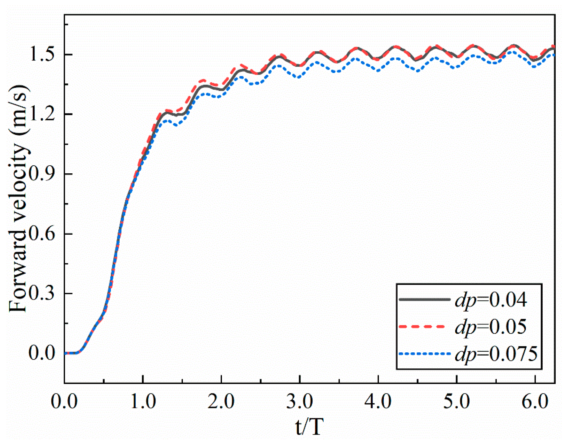
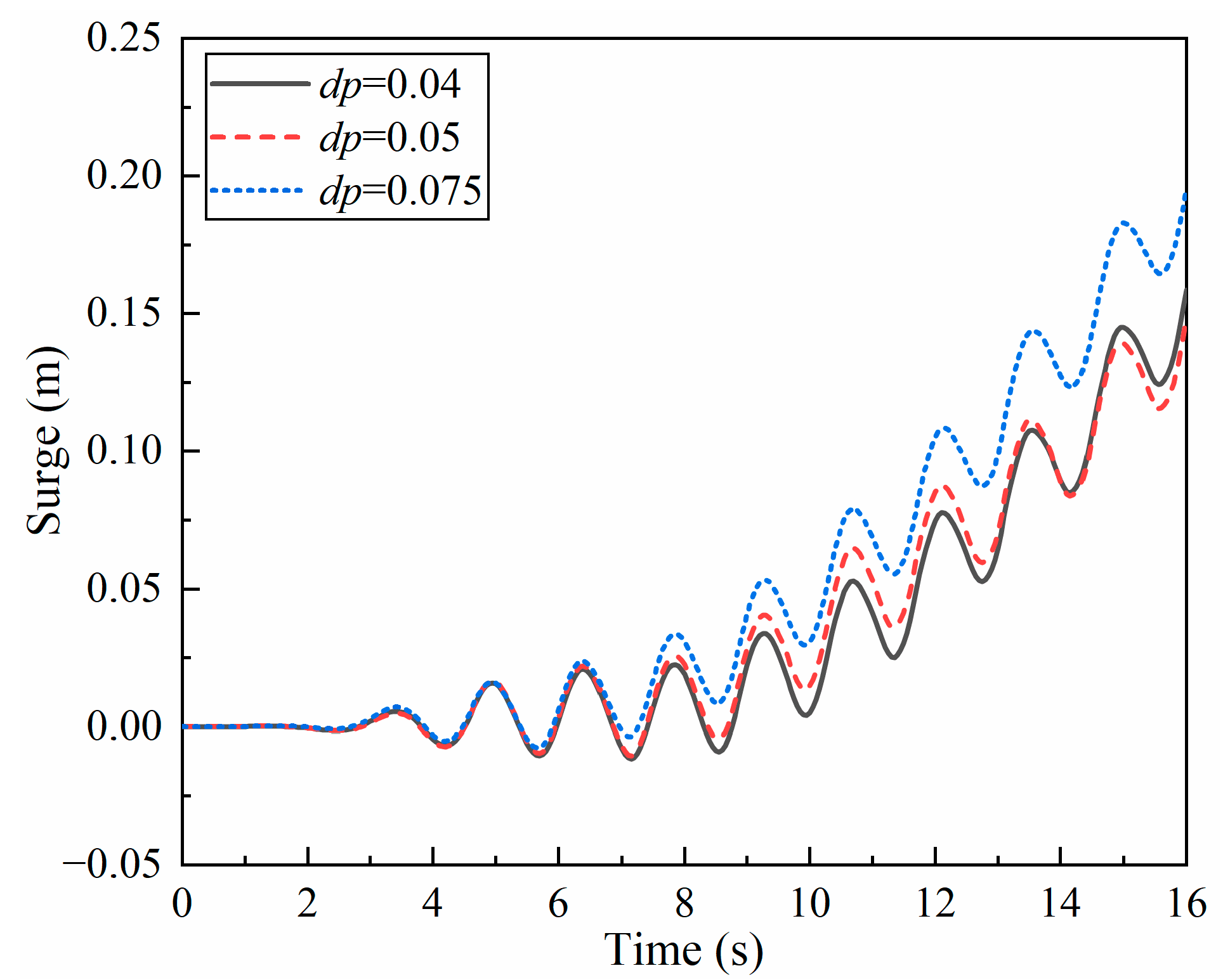
3.2. Resolution Verification

Figure 6 presents a comparison of the time histories of the forward velocity at different particle resolutions, specifically dp = 0.075, 0.05, and 0.04 m, with the undulation parameters set as a = 0.125, f = 1 Hz, and φ = 2π. Overall, the results for the three resolutions exhibit agreement with each other. However, it is noteworthy that the forward velocity at dp = 0.075 m experiences some attenuation compared to the other two resolutions, while dp = 0.005 m and dp = 0.004 m are closer, indicating the convergence of the results at a resolution of 0.005 m. Considering the computational efficiency and accuracy, a particle resolution of 0.005 m is selected for subsequent calculations of the self-propulsion of the multi-joint robotic fish.

The simulation domain of the energy harvesting model is different from the swimming model; thus, it is necessary to verify the resolution when studying the energy harvesting of multi-joint robotic fish. Three different resolutions, namely dp = 0.075, 0.05, and 0.04 m, are utilized to verify the resolution using a case with a damping coefficient of β = 0. The time-history surge of the multi-joint robotic fish at different resolutions is illustrated in Figure 7. It is evident that when dp = 0.075 m, the surge is relatively large, whereas greater consistency is observed in the results for dp = 0.005 and dp = 0.004 m. This suggests that the computational results are relatively accurate and have converged with a spatial resolution of dp = 0.005 m. In consideration of computational efficiency, a particle resolution of 0.005 m is employed for subsequent simulations of energy harvesting with the multi-joint robotic fish in this study.

4. Results and Discussion

Real fish generate thrust by bending their bodies through muscle contraction and relaxation, while multi-joint robotic fish imitate this process using rotating links. It is crucial to obtain a comprehensive understanding of the propulsion mechanism of multi-joint robotic fish from fluid dynamics. The flow field during the motion of multi-joint robotic fish is shown in Figure 8, where “JF” represents jet flow and the numbers indicate the sequence of jet flow generation. It is evident that the undulation of its tail continuously produces lateral jets during swimming, generating forward thrust through the reaction force of these jets. Due to the characteristic eel-like locomotion whereby the body amplitude gradually increases from the head to the tail, the flow velocity vectors around the head of the robotic fish are relatively smaller, whereas those around the tail are larger and exhibit a more complex flow field. The robotic fish primarily generates thrust through the oscillations of its tail, transferring this thrust through its joints to the head to overcome fluid resistance. Unlike real fish, multi-joint robotic fish are composed of multiple interconnected links with non-smooth surfaces, resulting in a more complex flow field their swimming.

4.1. Swimming Model and Swimming Efficiency of Multi-Joint Robotic Fish

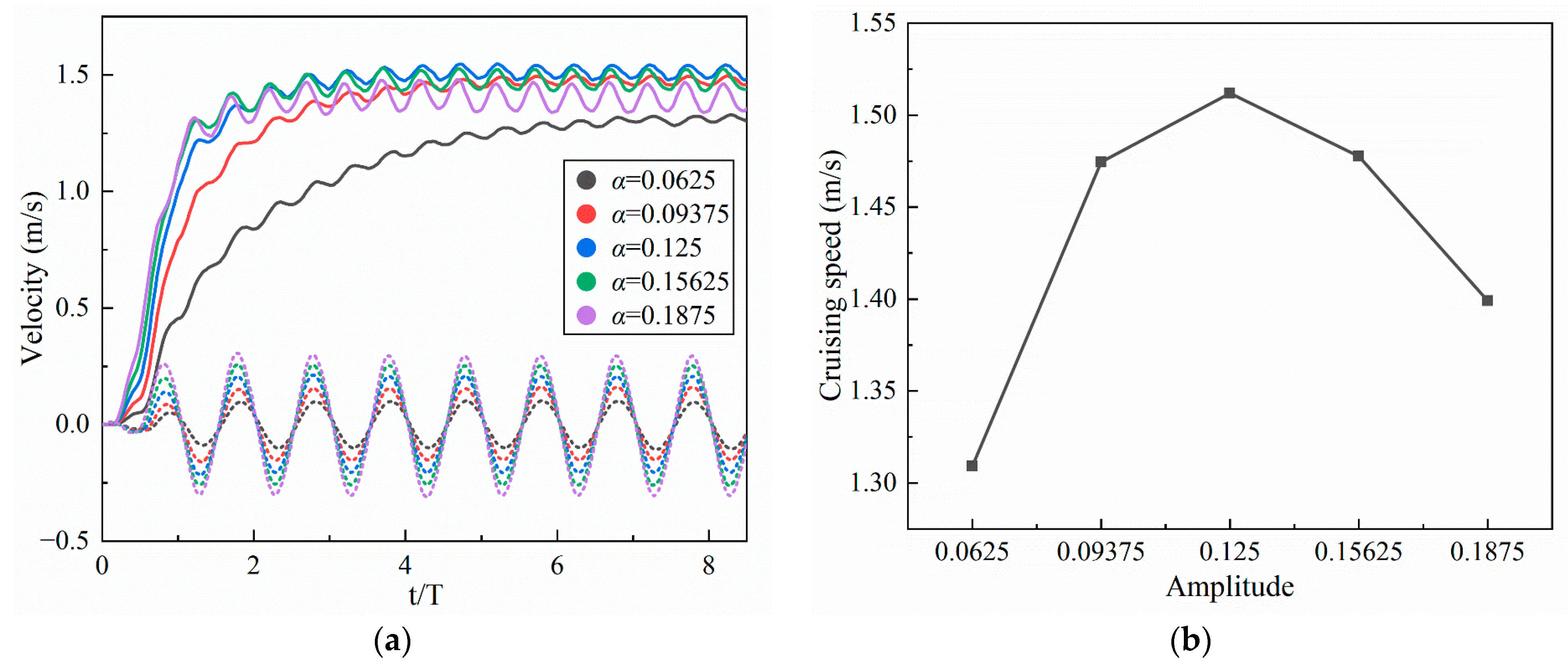
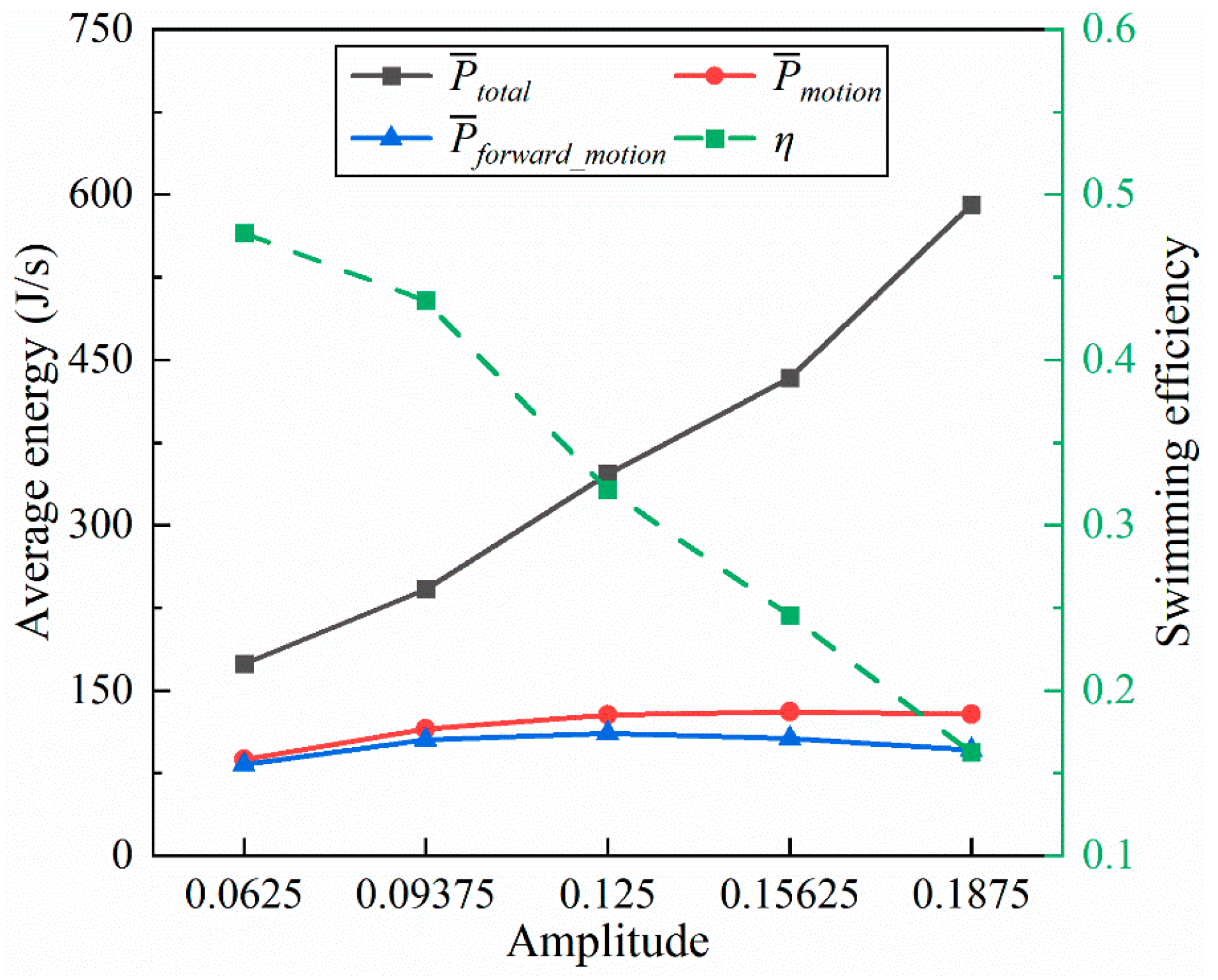
4.1.1. Amplitude Coefficient

The relationship between the amplitude and the velocity of the multi-joint robotic fish is illustrated in Figure 9a. It shows that as the amplitude increases, the lateral velocity of the robotic fish continuously increases. However, excessive lateral velocity can negatively impact its body stability. The time required to accelerate from rest to cruising speed gradually decreases and stabilizes, but the fluctuation amplitude of the forward velocity also increases accordingly. The cruising speed of the robotic fish can be computed using the time-averaged forward velocity from the last cycle. Figure 9b shows the relationship between cruising speed and amplitude. Although there is no significant difference in the cruising speed for different amplitudes, it is still evident that the cruising speed follows a trend of initially increasing and then decreasing with the amplitude. Combined with Figure 8, it can be inferred that the multi-joint robotic fish primarily relies on the undulation of its tail to generate thrust. As the amplitude increases, the lateral displacement of the tail also increases, resulting in a corresponding increase in fluid resistance in the forward direction. Consequently, the cruising speed decreases with increasing amplitude. At lower amplitudes, the lower energy of the tail jet results in weaker thrust and slower swimming speeds. Additionally, it is noteworthy that the maximum cruising speed corresponds to an amplitude coefficient of 0.125, which aligns with the swimming parameters of real eels in natural environments.

The average energy and efficiency of the multi-joint robotic fish vary with the amplitude, as shown in Figure 10. As the amplitude increases, the input power exhibits an approximately linear growth trend. However, the increase in average kinetic energy is relatively modest, remaining nearly constant when the amplitude surpasses coefficient 0.125. Moreover, the average forward kinetic energy initially increases and then decreases, similarly to the forward velocity. The gradual increase in the difference between the average kinetic energy and average forward kinetic energy indicates an increase in the energy used for lateral motion and link rotation. With the increase in average input power, the change in forward kinetic energy is relatively minor, resulting in a gradual decline in swimming efficiency and indicating that more input energy is dissipated into the surrounding fluid. A relatively smaller amplitude is a preferable choice. For example, taking the amplitude coefficients of 0.0625 and 0.125, doubling the amplitude results in a 0.2 m/s increase in cruising speed, but energy costs also double. Although lower amplitudes result in increased time for the robotic fish to reach cruising speed, they offer comparatively higher swimming efficiency.

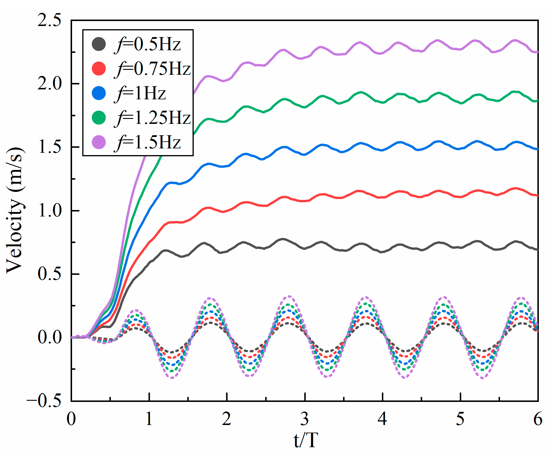
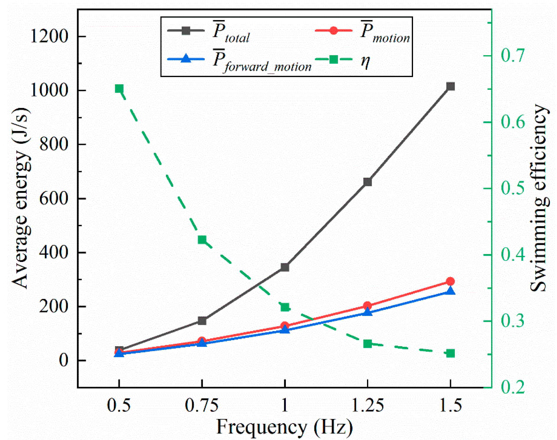
4.1.2. Frequency

The velocity of the multi-joint robotic fish at different frequencies is illustrated in Figure 11. As frequency increases, both the forward and lateral velocities of the robotic fish exhibit linear growth. Additionally, with the increase in frequency, the number of cycles required for the multi-joint robotic fish to reach the cruising speed increases accordingly. For instance, at a frequency of 0.5 Hz, it takes 1.5 cycles to enter the cruising state, whereas it requires four cycles to achieve the cruising speed at 1.5 Hz. At higher frequencies, the time required for the robotic fish to transition from rest to a cruising state decreases, and it demonstrates higher instantaneous acceleration during startup. Furthermore, the intensity of the tail jet is closely linked to the frequency; as the frequency increases, the velocity of the tail joint increases, resulting in a stronger tail jet. This interaction with the surrounding flow field enables the robotic fish to generate greater thrust and achieve a dynamic force balance at higher speeds.

Figure 12 illustrates the trends in the average energy and swimming efficiency of the multi-joint robotic fish at different frequencies. The results show that the average input energy of the multi-joint robotic fish exhibits nonlinear growth with a linear increase in frequency, and the growth rate gradually accelerates. Although the average kinetic energy also displays significant growth, its rate of increase is slower compared to the average input energy. This suggests that as the frequency increases, the proportion of energy used to overcome the surrounding fluid resistance in the total input energy gradually increases. Concurrently, combining Figure 11, it becomes apparent that the average energy costs of the multi-joint robotic fish laterally gradually increase, resulting in a widening discrepancy between its average kinetic energy and the average forward kinetic energy. The swimming efficiency indicates that in all simulated conditions, the maximum swimming efficiency can reach 0.65. As frequency increases, swimming efficiency gradually decreases, with the rate of change gradually slowing down. Therefore, when selecting the parameter frequency, a balance needs to be achieved between the maximum speed and the swimming efficiency. However, taking frequencies of 0.5 Hz and 1 Hz as examples, although doubling the frequency results in the doubling of the cruising speed, the average input energy at 1 Hz is 9.25 times that at 0.5 Hz. From the perspective of energy self-sufficiency in robotic fish, for which its energy is derived from waves, low-frequency motion aligns better with the goal of efficient energy utilization.

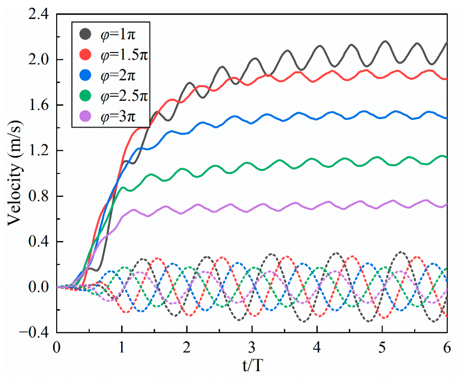
4.1.3. Phase

The phase mainly affects the body wavelength of the multi-joint robotic fish during swimming. When the phase is φ = π, 1.5π, 2π, 2.5π, and 3π, the corresponding body wavelengths are 2L_c, 4/3L_c, L_c, 4/5L_c, and 2/3L_c, respectively. Taking φ = π and φ = 2π as examples, when φ = π, the body of the robotic fish exhibits a gradually increasing half sine wave shape, whereas when φ = 2π, the body gradually displays an increasing full sine wave shape during swimming. The relationship between the velocity and the phase of the multi-joint robotic fish is illustrated in Figure 13. When φ = π, the forward velocity is close to that at φ = 1.5π, whereas for other phases, the forward velocity decreases linearly with the increasing phase. Additionally, the time required for the multi-joint robotic fish to reach the cruising speed gradually decreases. Due to the variation in phase for different phases of the multi-joint robotic fish, there is a phase difference of T/4 on the velocity curve. Additionally, the lateral velocity gradually decreases with increasing amplitude. Combined with Figure 8, the flow fields of the robotic fish with different wavelengths are illustrated in Figure 14. Taking φ = π and φ = 3π as examples, when φ = π, the body wave of the robotic fish generates a strong jet flow in the flow field, resulting in a faster swimming speed. When φ = 3π, the increase in the body wave of the robotic fish results in a relatively smaller disturbance to the fluid caused by its undulating motion. Meanwhile, the thrust and lift generated by the tail flapping are partially balanced by other parts of the body, resulting in a decrease in both the forward and the lateral velocity.

The variation in the average energy and swimming efficiency of the multi-joint robotic fish with respect to the phase is illustrated in Figure 15. The average input energy exhibits an initially decreasing trend followed by an increase, reaching its minimum at φ = 2π. Both the average kinetic energy and the average forward kinetic energy decrease synchronously with the increase in phase, with their curves being approximately parallel. As the phase increases from π to 2π, the average input energy decreases rapidly, while the average forward kinetic energy decreases slowly, resulting in a slight decrease in swimming efficiency. However, as the phase increases from 2π to 3π, the average forward kinetic energy gradually decreases whereas the input power increases, resulting in a rapid decline in swimming efficiency. Combined with Figure 14b, it can be observed that although the link movements are complex, the thrust and lift generated by the body are largely offset. The increase in the average input energy does not effectively translate into forward propulsion. From the perspectives of swimming efficiency and stability, φ = 2π is the optimal choice for the multi-joint self-propelled robotic fish.

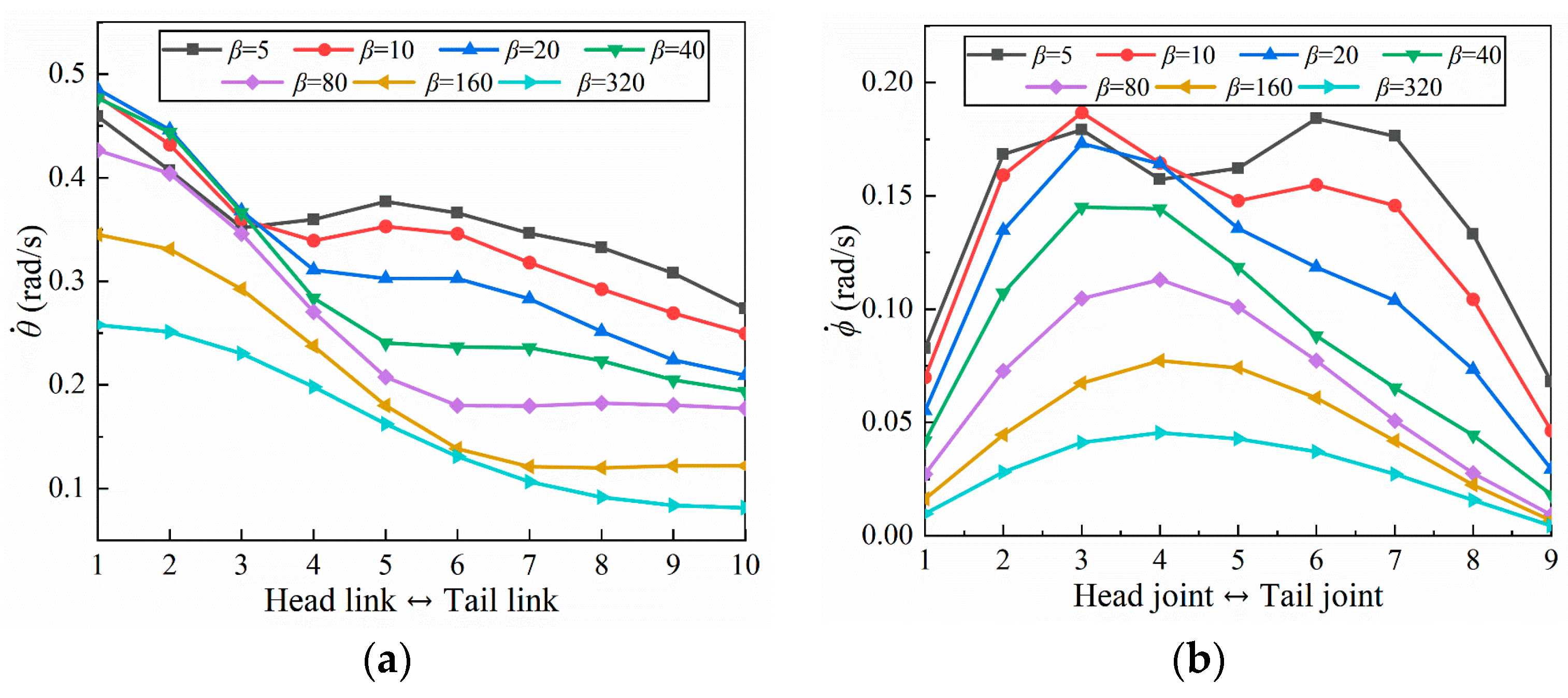
4.2. Energy Harvesting Model and Power in Waves

In the energy-harvesting mode, the relative rotation of adjacent links under the action of waves drives the motor at the joint to generate electrical energy. However, the driving moment of the motor exists in the form of a resistance moment for the robotic fish. The introduction of different damping coefficients (β) is essential in studying the impact of the PTO system on energy harvesting. To observe the relationship between the power and damping coefficient, a logarithmic analysis of the damping coefficient is employed. The damping coefficients in this study are 5, 10, 20, 40, 80, 160, and 320, with corresponding logarithms of 0.699, 1, 1.301, 1.602, 1.903, 2.204, and 2.505.

The energy harvested by the multi-joint robotic fish is directly related to the rotational angular velocity of its links. To clearly reflect the relationship between the angular velocity, link position, and damping coefficient, the root mean square of the angular velocity is used to represent the angular velocity of each link of the multi-joint robotic fish. The difference in angular velocity between adjacent links is also treated using the same method as follows:

$$\widehat{\dot{\theta }}=\sqrt{\frac{1}{k}\sum _{i=1}^k {\dot{\theta }}_i^2}$$

(29)

where $\widehat{\dot{\theta }}$ is the root mean square of the angular velocity, k is the total number of steps, and $\dot{{\theta }_i}$ is the angular velocity of the link at step i.

Figure 16 illustrates the variation in the angular velocity of the links and the difference in angular velocity between adjacent links along the multi-joint robotic fish, from the head to the tail, under different damping coefficients. With an increase in the damping coefficient, the resisting moment that the robotic fish must counteract to rotate at the same angle also increases. Consequently, under constant wave loading, the angular velocity of each link decreases, as shown in Figure 16a. The wave first contacts the head of the robotic fish, and its energy is absorbed by the fish during propagation, resulting in significantly higher angular velocities at the head joints compared to the tail joints. The variation in the difference in angular velocity between adjacent links, from the head to the tail of the robotic fish, under different damping coefficients is depicted in Figure 16b. The difference in angular velocity between adjacent joints exhibits first an increasing trend and then decreases from the head to the tail of the fish. For lower damping coefficients (β = 5–40 Nms/rad), the peak occurs at the third joint, whereas for higher damping coefficients (β = 80–320 Nms/rad), the peak shifts to the fourth joint. With the increase in the damping coefficient, the difference in the angular velocity between adjacent joints at each joint decreases, and this is consistent with the results shown in Figure 16a.

The relationship between the average harvested power and the damping coefficient of the PTO system is shown in Figure 17. It can be observed that the harvested power exhibits an initially increasing trend that then decreases. The logarithm of the damping coefficient corresponding to the peak of the average harvested power is 1.903 Nms/rad, with the associated damping coefficient being 80 Nms/rad. Combining Equations (24) and (26) with the information from Figure 16, it can be observed that when the damping coefficient is small, the larger relative rotation angles between the links result in smaller torques driving the motor’s rotation, resulting in lower harvested power. Conversely, when the damping coefficient is too large, although the resistance moment is high, the relative motion between the joints is minimal, also resulting in similarly low harvested power. The damping coefficient must be set to an appropriate value for the torque and motion of the links to achieve balance and maximize energy harvesting. Therefore, based on the aforementioned analysis, the most suitable damping coefficient for energy harvesting in the robotic fish is determined to be 80 Nms/rad. The energy-harvesting efficiency for the optimal damping coefficient is calculated to be 0.163, indicating that 16.3% of the wave energy can be converted into electrical energy to drive the self-propelled robotic fish in the wave environment studied. This efficiency analysis provides a reference for the design of self-sufficient robotic fish.

Figure 18 illustrates the time history of the surge, heave, and pitch of the multi-joint robotic fish in waves. The left shows the case in which the damping coefficient is β = 0 Nms/rad (a–c), whereas the right is the scenario in which the damping coefficient is β = 80 Nms/rad (d–f). As shown in Figure 18a, in the absence of damping, the surge exhibits oscillatory behavior, with greater amplitudes in the positive direction than in the negative direction, resulting in the overall forward movement of the robotic fish. However, with a damping coefficient of 80 Nms/rad, the motion is unidirectional in the positive direction, without any motion in the negative direction, as shown in Figure 18d. Figure 19b,e show the heave with and without damping, respectively. In the absence of damping, the heaving amplitudes of each link are similar; however, when the damping coefficient is 80 Nms/rad, the amplitudes of all links are relatively similar, except for links 1 and 2, and there are phase differences between different positions of the links. The pitches of the links with and without damping are shown in Figure 19c,f. In the absence of damping, although the pitch of each link exhibits periodic variations, it does not strictly follow a sinusoidal curve due to the influence of inter-joint interaction forces. However, with damping, the pitch follows a sinusoidal pattern. The pitching amplitude gradually decreases from the head to the fourth link, while the pitching amplitudes of other links are approximately equal.

Figure 19 shows the velocity field of a multi-joint robotic fish in a full cycle. In the absence of damping between the joints, the robotic fish deforms freely with the undulation of the waves, and the velocity field on the body is consistent with the surrounding fluid velocity. Due to the smaller length of the robotic fish compared to the wavelength, the velocity vectors are unbalanced in the horizontal direction, while fluid particles spiral forward along the direction of wave propagation, resulting in the horizontal oscillatory motion of the robotic fish. The velocity vectors on both sides of the robotic fish are similar in magnitude and exhibit no significant decay, resulting in near-identical amplitudes of motion at each joint in the vertical direction. For the same wave environment, when the damping coefficient between the joints is 80 Nms/rad, it can be clearly observed that the velocity vector on the right side of the robotic fish experiences significant attenuation compared to the left side. As the wave propagates to the right, the wave peak causes the head of the robotic fish to undergo larger vertical displacement. At the same time, the energy of the wave is harvested by the joints, reducing the wave height, and the vertical displacement and rotation angle of the tail link are also correspondingly reduced, showing an overall fluctuating motion.

4.3. Feasibility Analysis of Energy Self-Sufficiency

According to Section 4.1, it can be determined that the undulation frequency is the primary variable affecting the swimming efficiency, followed by the amplitude, and the phase is the third key variable. For the robotic fish studied in this work, its energy harvesting capability primarily relies on the surrounding wave environment. Therefore, efficient energy utilization during swimming is crucial in achieving energy self-sufficiency. Studies have demonstrated that reducing both the undulation frequency and amplitude while maintaining a complete body wavelength can lead to a balance between swimming efficiency and stability. Therefore, we select an amplitude coefficient of a = 0.0625, frequency of f = 0.5Hz, and phase of φ = 2π as undulation parameters for verification. The simulated forward velocity and lateral velocity of the robotic fish are shown in Figure 20. Under these motion parameters, although it takes six undulation cycles to reach the cruising speed, the swimming velocity reaches 0.6 m/s, with a lateral velocity of only 0.05 m/s. The average energy and swimming efficiency of the multi-joint robotic fish during swimming are shown in

Table 1. Average energy and swimming efficiency under high-swimming-efficiency parameters.

${\overline{\mathit{P}}}_{\mathit{t}\mathit{o}\mathit{t}\mathit{a}\mathit{l}}$ (J/s)	${\overline{\mathit{P}}}_{\mathit{m}\mathit{o}\mathit{t}\mathit{i}\mathit{o}\mathit{n}}$ (J/s)	${\overline{\mathit{P}}}_{\mathit{f}\mathit{o}\mathit{r}\mathit{w}\mathit{a}\mathit{r}\mathit{d}\mathit{m}\mathit{o}\mathit{t}\mathit{i}\mathit{o}\mathit{n}}$ (J/s)	${\mathit{\eta }}_{\mathit{m}}$
23.3	18.7	17.53	0.75

. It can be observed that the average energy cost is 23.3 W, with the majority of the energy being converted into kinetic energy for the forward motion of the robotic fish, while only a small fraction of the energy is dissipated in the surrounding flow field, resulting in swimming efficiency as high as 0.75.

The power harvested by the multi-joint robotic fish is 4 W in a wave environment with a wave height of 0.1 m and a wavelength of 3 m. Combining Figure 20 and Table 1, it can be calculated that the energy harvested by the robotic fish floating in the wave environment studied for 24 h is sufficient to support its swimming for 4.12 h, covering a distance of 8899 m. Importantly, the wave height examined in this study is only 0.1 m, which reflects Level 1 sea conditions. As the wave height increases, power harvesting can be further improved. The study demonstrates the enormous potential for underwater robots to achieve energy self-sufficiency through wave energy harvesting.

5. Conclusions

In this study, the energy costs and the energy harvesting of multi-joint robotic fish are numerically simulated using a coupled DualSPHysics and Chrono method. The relationship between different undulation parameters and swimming performance is studied, such as motion speeds, energy costs, and swimming efficiency, and the influence of the PTO system on energy harvesting is examined. Additionally, a high-efficiency swimming mode is proposed, and its energy self-sufficiency performance is evaluated in conjunction with the energy-harvesting capability. The main conclusions are as follows.

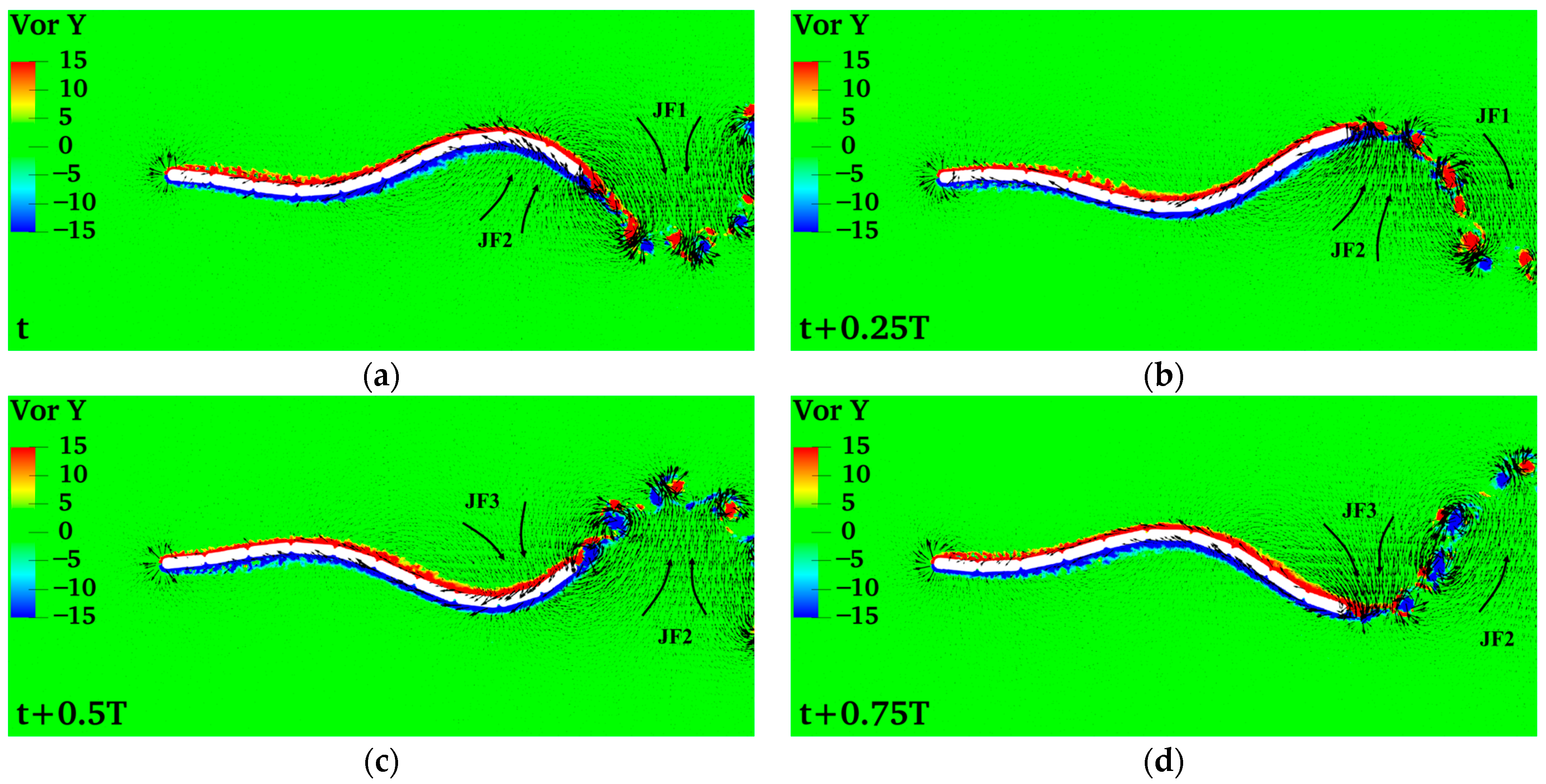
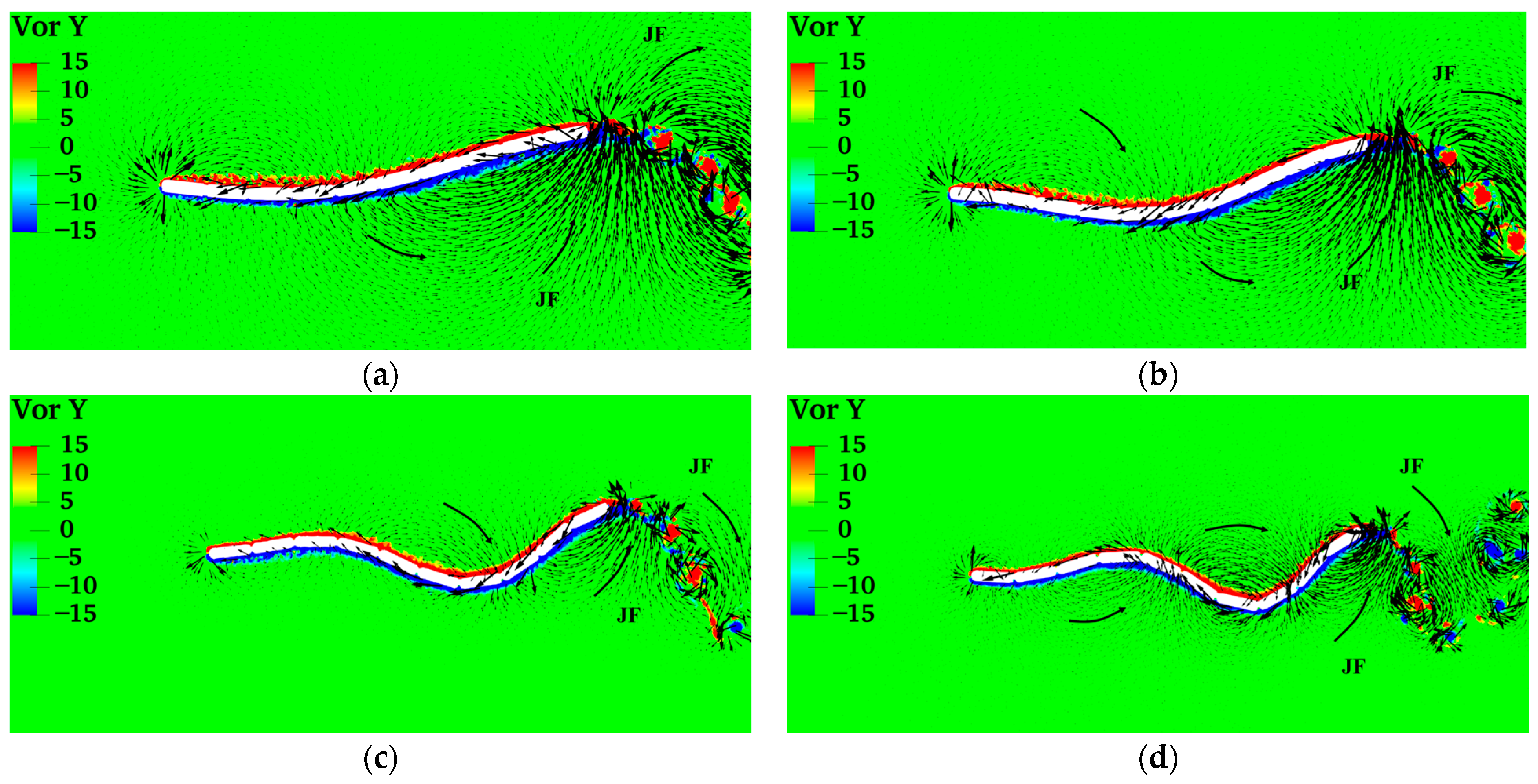
• Inspired by the locomotion of eels, the thrust of multi-joint robotic fish primarily arises from the reactive force of the jet flow generated by tail oscillations. The undulation parameters, namely, the amplitude, frequency, and phase, of the robotic fish are crucial factors influencing the strength of the jet flow, and they strongly affect the velocity, energy costs, and swimming efficiency of the fish. It is observed that the frequency is the primary variable affecting both the energy costs and efficiency, followed by the amplitude and phase. Although low frequencies and amplitudes, along with phase adjustments to maintain a complete wavelength, could effectively reduce energy costs and promote body stability, there is a compromise in the forward speed.
• PTO systems with different damping coefficients affect the wave-induced motion of robotic fish by applying a resistance moment at the joints, thereby impacting the power and efficiency of energy harvesting. It is observed that determining the appropriate damping coefficient for multi-joint robotic fish is important for balancing body motion and joint resistance moment during energy harvesting, thereby maximizing the harvested energy from waves. In the wave environment in this study, the maximum power output can reach 4 W under optimal damping coefficients.
• The energy harvesting of multi-joint robotic fish is determined by the damping coefficients and environmental factors. Therefore, the key to achieving energy self-sufficiency for multi-joint robotic fish lies in adjusting the undulation parameters to reduce energy costs and enhance swimming efficiency. Under the examined conditions of wave energy harvesting and undulation parameters, the ratio of the average energy harvested by the multi-joint robotic fish to the average energy cost is 1:5.8, demonstrating that energy self-sufficiency is feasible.
• This research demonstrates that it is feasible for multi-joint robotic fish to achieve energy self-sufficiency in wave environments, and there is great potential for development. Additionally, it provides an effective and sustainable solution for the long-term operation of underwater robots.

In the future, the authors will investigate the energy self-sufficiency performance of multi-joint robotic fish with different shapes of links, as well as the impact of different wave environments on the energy-harvesting efficiency and power of the fish. Additionally, the conclusions of this study will be validated through experimental methods.

References

- Breder, C.M. The Locomotion of Fishes. Zoologica 1926, 4, 159–297. [Google Scholar] [CrossRef]
- Van Ginneken, V.; Antonissen, E.; Müller, U.K.; Booms, R.; Eding, E.; Verreth, J.; Van Den Thillart, G. Eel Migration to the Sargasso: Remarkably High Swimming Efficiency and Low Energy Costs. J. Exp. Biol. 2005, 208, 1329–1335. [Google Scholar] [CrossRef] [PubMed]
- Gillis, G.B. Undulatory Locomotion in Elongate Aquatic Vertebrates: Anguilliform Swimming since Sir James Gray. Am. Zool. 1996, 36, 656–665. [Google Scholar] [CrossRef]
- Gray, J. Studies in Animal Locomotion: I. The Movement of Fish with Special Reference to the Eel. J. Exp. Biol. 1933, 10, 88–104. [Google Scholar] [CrossRef]
- Fish, F.E.; Lauder, G.V. Passive and Active Flow Control by Swimming Fishes and Mammals. Annu. Rev. Fluid Mech. 2006, 38, 193–224. [Google Scholar] [CrossRef]
- Müller, U.K.; Van Leeuwen, J.L. Undulatory Fish Swimming: From Muscles to Flow. Fish Fish. 2006, 7, 84–103. [Google Scholar] [CrossRef]
- Triantafyllou, M.S.; Triantafyllou, G.S.; Yue, D.K.P. Hydrodynamics of Fishlike Swimming. Annu. Rev. Fluid Mech. 2000, 32, 33–53. [Google Scholar] [CrossRef]
- Minami, M.; Jingyu, G.; Mae, Y. Chaos-Driving Robotic Intelligence for Catching Fish. In Proceedings of the 2007 IEEE International Conference on Robotics and Automation, Rome, Italy, 10–14 April 2007; pp. 85–91. [Google Scholar]
- Carling, J.; Williams, T.L.; Bowtell, G. Self-Propelled Anguilliform Swimming: Simultaneous Solution of the Two-Dimensional Navier–Stokes Equations and Newton’s Laws of Motion. J. Exp. Biol. 1998, 201, 3143–3166. [Google Scholar] [CrossRef] [PubMed]
- Taylo, G.I. Analysis of the Swimming of Long and Narrow Animals. Proc. R. Soc. Lond. Ser. A Math. Phys. Sci. 1952, 214, 158–183. [Google Scholar] [CrossRef]
- Lighthill, M.J. Large-Amplitude Elongated-Body Theory of Fish Locomotion. Proc. R. Soc. Lond. Ser. B Biol. Sci. 1971, 179, 125–138. [Google Scholar] [CrossRef]
- McIsaac, K.A.; Ostrowski, J.P. Motion Planning for Anguilliform Locomotion. IEEE Trans. Robot. Autom. 2003, 19, 637–652. [Google Scholar] [CrossRef]
- Boyer, F.; Porez, M.; Khalil, W. Macro-Continuous Computed Torque Algorithm for a Three-Dimensional Eel-like Robot. IEEE Trans. Robot. 2006, 22, 763–775. [Google Scholar] [CrossRef]
- Ekeberg, Ö. A Combined Neuronal and Mechanical Model of Fish Swimming. Biol. Cybern. 1993, 69, 363–374. [Google Scholar] [CrossRef]
- Wiens, A.J.; Nahon, M. Optimally Efficient Swimming in Hyper-Redundant Mechanisms: Control, Design, and Energy Recovery. Bioinspiration Biomim. 2012, 7, 046016. [Google Scholar] [CrossRef] [PubMed]
- Khalil, W.; Gallot, G.; Boyer, F. Dynamic Modeling and Simulation of a 3-D Serial Eel-Like Robot. IEEE Trans. Syst. Man Cybern. C 2007, 37, 1259–1268. [Google Scholar] [CrossRef]
- Candelier, F.; Porez, M.; Boyer, F. Note on the Swimming of an Elongated Body in a Non-Uniform Flow. J. Fluid Mech. 2013, 716, 616–637. [Google Scholar] [CrossRef]
- Kelasidi, E.; Pettersen, K.Y.; Gravdahl, J.T. Modeling of Underwater Snake Robots. In Proceedings of the 2014 IEEE International Conference on Robotics and Automation (ICRA), Hong Kong, China, 31 May–7 June 2014; pp. 4540–4547. [Google Scholar] [CrossRef]
- Mikołajczyk, T.; Mikołajewski, D.; Kłodowski, A.; Łukaszewicz, A.; Mikołajewska, E.; Paczkowski, T.; Macko, M.; Skornia, M. Energy Sources of Mobile Robot Power Systems: A Systematic Review and Comparison of Efficiency. Appl. Sci. 2023, 13, 7547. [Google Scholar] [CrossRef]
- Prudell, J.; Stoddard, M.; Amon, E.; Brekken, T.K.A.; Von Jouanne, A. A Permanent-Magnet Tubular Linear Generator for Ocean Wave Energy Conversion. IEEE Trans. Ind. Appl. 2010, 46, 2392–2400. [Google Scholar] [CrossRef]
- Sodano, H.A.; Park, G.; Inman, D.J. Estimation of Electric Charge Output for Piezoelectric Energy Harvesting. Strain 2004, 40, 49–58. [Google Scholar] [CrossRef]
- Wang, J.; Tang, L.; Zhao, L.; Zhang, Z. Efficiency Investigation on Energy Harvesting from Airflows in HVAC System Based on Galloping of Isosceles Triangle Sectioned Bluff Bodies. Energy 2019, 172, 1066–1078. [Google Scholar] [CrossRef]
- Michelin, S.; Doare, O. Energy Harvesting Efficiency of Piezoelectric Flags in Axial Flows. J. Fluid Mech. 2013, 714, 489–504. [Google Scholar] [CrossRef]
- Hirt, C.W.; Nichols, B.D. Volume of Fluid (VOF) Method for the Dynamics of Free Boundaries. J. Comput. Phys. 1981, 39, 201–225. [Google Scholar] [CrossRef]
- Lakzian, E.; Ramezani, M.; Shabani, S.; Salmani, F.; Majkut, M.; Kim, H.D. The Search for an Appropriate Condensation Model to Simulate Wet Steam Transonic Flows. Int. J. Numer. Methods Heat Fluid Flow 2023, 33, 2853–2876. [Google Scholar] [CrossRef]
- Dalrymple, R.A.; Rogers, B.D. Numerical Modeling of Water Waves with the SPH Method. Coast. Eng. 2006, 53, 141–147. [Google Scholar] [CrossRef]
- Monaghan, J.J.; Kos, A.; Issa, N. Fluid Motion Generated by Impact. J. Waterw. Port Coast. Ocean. Eng. 2003, 129, 250–259. [Google Scholar] [CrossRef]
- Falcão, A.F. Wave Energy Utilization: A Review of the Technologies. Renew. Sustain. Energy Rev. 2010, 14, 899–918. [Google Scholar] [CrossRef]
- McCormick, M.E. Ocean Wave Energy Conversion; Courier Corporation: Chelmsford, MA, USA, 2013. [Google Scholar]
- Salter, S.H. World Progress in Wave Energy—1988. Int. J. Ambient. Energy 1989, 10, 3–24. [Google Scholar] [CrossRef]
- Dalton, G.J.; Alcorn, R.; Lewis, T. Case Study Feasibility Analysis of the Pelamis Wave Energy Convertor in Ireland, Portugal and North America. Renew. Energy 2010, 35, 443–455. [Google Scholar] [CrossRef]
- Dong, E.; Yan, Q.; Zhang, S.; Yang, J. Self-Powered System of Articulated Bionic Robotic Fish Using Wave Energy Harvesting. Robot 2009, 31, 501–505. [Google Scholar]
- Zhu, W.; Wang, X.; Xu, M.; Yang, J.; Si, T.; Zhang, S. A Wave Energy Conversion Mechanism Applied in Robotic Fish. In Proceedings of the 2013 IEEE/ASME International Conference on Advanced Intelligent Mechatronics, Wollongong, NSW, Australia, 9–12 July 2013; pp. 319–324. [Google Scholar] [CrossRef]
- Ruffini, G.; Briganti, R.; De Girolamo, P.; Stolle, J.; Ghiassi, B.; Castellino, M. Numerical Modelling of Flow-Debris Interaction during Extreme Hydrodynamic Events with DualSPHysics-CHRONO. Appl. Sci. 2021, 11, 3618. [Google Scholar] [CrossRef]
- Domínguez, J.M.; Fourtakas, G.; Altomare, C.; Canelas, R.B.; Tafuni, A.; García-Feal, O.; Martínez-Estévez, I.; Mokos, A.; Vacondio, R.; Crespo, A.J.C.; et al. DualSPHysics: From Fluid Dynamics to Multiphysics Problems. Comput. Part. Mech. 2022, 9, 867–895. [Google Scholar] [CrossRef]
- Lo, E.Y.; Shao, S. Simulation of Near-Shore Solitary Wave Mechanics by an Incompressible SPH Method. Appl. Ocean Res. 2002, 24, 275–286. [Google Scholar] [CrossRef]
- Fourtakas, G.; Dominguez, J.M.; Vacondio, R.; Rogers, B.D. Local Uniform Stencil (LUST) Boundary Condition for Arbitrary 3-D Boundaries in Parallel Smoothed Particle Hydrodynamics (SPH) Models. Comput. Fluids 2019, 190, 346–361. [Google Scholar] [CrossRef]
- Tasora, A.; Anitescu, M. A Matrix-Free Cone Complementarity Approach for Solving Large-Scale, Nonsmooth, Rigid Body Dynamics. Comput. Methods Appl. Mech. Eng. 2011, 200, 439–453. [Google Scholar] [CrossRef]
- Canelas, R.B.; Domínguez, J.M.; Crespo, A.J.C.; Gómez-Gesteira, M.; Ferreira, R.M.L. A Smooth Particle Hydrodynamics Discretization for the Modelling of Free Surface Flows and Rigid Body Dynamics. Numer. Methods Fluids 2015, 78, 581–593. [Google Scholar] [CrossRef]
- Brito, M.; Canelas, R.B.; García-Feal, O.; Domínguez, J.M.; Crespo, A.J.C.; Ferreira, R.M.L.; Neves, M.G.; Teixeira, L. A Numerical Tool for Modelling Oscillating Wave Surge Converter with Nonlinear Mechanical Constraints. Renew. Energy 2020, 146, 2024–2043. [Google Scholar] [CrossRef]
- Tasora, A.; Serban, R.; Mazhar, H.; Pazouki, A.; Melanz, D.; Fleischmann, J.; Taylor, M.; Sugiyama, H.; Negrut, D. Chrono: An Open Source Multi-Physics Dynamics Engine. In High Performance Computing in Science and Engineering; Lecture Notes in Computer Science; Springer International Publishing: Cham, Switzerland, 2016; Volume 9611, pp. 19–49. ISBN 978-3-319-40360-1. [Google Scholar]
- Canelas, R.B.; Brito, M.; Feal, O.G.; Domínguez, J.M.; Crespo, A.J.C. Extending DualSPHysics with a Differential Variational Inequality: Modeling Fluid-Mechanism Interaction. Appl. Ocean Res. 2018, 76, 88–97. [Google Scholar] [CrossRef]
- Kern, S.; Koumoutsakos, P. Simulations of Optimized Anguilliform Swimming. J. Exp. Biol. 2006, 209, 4841–4857. [Google Scholar] [CrossRef] [PubMed]
- Bua, L.; Magis, B.; Ronsse, R.; Chatelain, P.; Bernier, C.; Jeanmart, H. Swimming Eel-like Robot: Design Improvement and Control. Master’s Thesis, Ecole polytechnique de Louvain, Louvain-la-Neuve, Belgium, 2018. [Google Scholar]
- Kelasidi, E.; Pettersen, K.Y.; Gravdahl, J.T. Energy Efficiency of Underwater Snake Robot Locomotion. In Proceedings of the 2015 23rd Mediterranean Conference on Control and Automation (MED), Torremolinos, Spain, 16–19 June 2015; pp. 1124–1131. [Google Scholar] [CrossRef]
- Tagliafierro, B.; Martínez-Estévez, I.; Crego-Loureiro, C.; Domínguez, J.M.; Crespo, A.J.C.; Coe, R.G.; Bacelli, G.; Gómez-Gesteira, M.; Viccione, G. Numerical Modeling of Moored Floating Platforms for Wave Energy Converters Using DualSPHysics. Ocean. Eng. 2022, 5, V05AT06A016. [Google Scholar] [CrossRef]
- Brooke, J. Wave Energy Conversion; Elsevier: Amsterdam, The Netherlands, 2003. [Google Scholar]
- Lu, K.; Xie, Y.H.; Zhang, D. Numerical Study of Large Amplitude, Nonsinusoidal Motion and Camber Effects on Pitching Airfoil Propulsion. J. Fluids Struct. 2013, 36, 184–194. [Google Scholar] [CrossRef]
- Ren, B.; He, M.; Dong, P.; Wen, H. Nonlinear Simulations of Wave-Induced Motions of a Freely Floating Body Using WCSPH Method. Appl. Ocean Res. 2015, 50, 1–12. [Google Scholar] [CrossRef]
- Feng, H.; Wang, Z.; Todd, P.A.; Lee, H.P. Simulations of Self-Propelled Anguilliform Swimming Using the Immersed Boundary Method in OpenFOAM. Eng. Appl. Comput. Fluid Mech. 2019, 13, 438–452. [Google Scholar] [CrossRef]