Article

Infragravity Wave Oscillation Forecasting in a Shallow Estuary

1
Department of Civil and Environmental Engineering, University of California, Los Angeles, CA 90095, USA
2
Scripps Institution of Oceanography, University of California San Diego, La Jolla, CA 92093, USA
*
Author to whom correspondence should be addressed.
These authors contributed equally to this work.
J. Mar. Sci. Eng. 2024, 12(4), 672; https://doi.org/10.3390/jmse12040672
Submission received: 13 March 2024 / Revised: 7 April 2024 / Accepted: 11 April 2024 / Published: 18 April 2024
(This article belongs to the Section Coastal Engineering)

Abstract

:
Infragravity (IG) waves are low-frequency water waves, which can propagate into harbors and estuaries, affecting currents and sediment transport processes. Understanding and predicting IG oscillations inside harbors and estuaries is critical to coastal management and estimating future resilience to climate change impacts. High-resolution water level and flow velocity observations collected within Seal Beach Wildlife Refuge in Southern California are analyzed for IG energy related to atmospheric parameters, water levels, and offshore wave conditions. A proof of concept approach for predicting infragravity oscillations within an estuary using machine learning (ML) is presented.

1. Introduction

Estuaries are partially enclosed coastal water bodies that exhibit strong longitudinal density gradients. Traditionally, estuaries are frequently described as regions where freshwater inputs converge and mix with saline oceanic waters. However, many estuaries have minimal and/or intermittent inflow and are marine-process (i.e., waves, tides, infragravity) dominated [1]. Estuaries can support extensive marsh, tidal flat, and subtidal habitats; provide carbon sequestration and resilience to flooding from storms and sea level rise; and are valuable recreational spaces [2,3]. Small, low inflow estuaries are particularly dynamic coastal systems, due to the combination of tides, waves, and the presence of shallow channels, intertidal regions, and active morphodynamics [4,5,6]. These unique estuarine systems will be substantially impacted by climate change. The management of these important systems is a major global challenge [7].
Infragravity (IG) waves are surface ocean waves with periods between 25 and 300 s [8], and they are known to impact small harbors and estuaries [9,10]. Free IG waves may be amplified by resonance and induce large oscillations (seiches) and ship motions in closed or semi-enclosed water bodies, which have implications for navigation, sediment transport, and turbidity [11]. Basin resonant modes, and their ability to trap IG waves, are defined by a basin’s geometry and water depth; accordingly, resonance behavior may vary with tidal water levels [12,13,14]. Multiple observational studies and numerical simulations have shown that the strength of IG motions is correlated with the offshore wave conditions [8,15,16,17,18,19,20,21]. The relationship between short wave parameters and IG waves has been investigated in the past [22,23,24]. However, while incident wave observations are frequently recorded, IG measurements are less common.
The morphology of tidal inlets, characterized by the presence of an ebb-tidal delta, a main channel, and secondary channels, differs from that of beaches. As a result, IG wave generation, propagation, and dissipation mechanisms in tidal inlets may be quite different from those on beaches. For example, on beaches all incoming IG wave energy is dissipated or reflected. In contrast, in estuarine environments a portion of the IG energy may propagate through the channels and into the estuary interior [3,4,19,25]. Numerical results have suggested that the break point and the long bound wave shoaling mechanisms can contribute significantly to the generation of IG waves in the inlet [25]. Williams and Stacey [19] performed field measurements at a shallow inlet in Northern California and observed fluctuations in water levels and current velocities of the order of a minute, which were identified as IG waves. Bowers [26] found an inverse correlation between the tidal level and IG energy, and Bertin et al. [20] noted that the IG levels in shallow systems are smaller during the ebb phase due to the blocking effects of opposing currents. Investigations by Harvey et al. [4], Williams and Stacey [19], Bertin et al. [20] reveal that IG orbital motion magnitudes inside estuaries may be similar to tidal velocities. IG waves have been shown to induce significant currents and sediment transport changes [4,6,20,27,28]. For example, Mendes et al. [3] showed that the IG oscillations inside a studied marsh results in sediment accretion in specific areas, potentially altering inlet morphology and leading to estuary mouth closures [4,29]. A comprehensive understanding of IG propagation into estuaries is critical for quantifying future climate change impacts arising from increasing sea levels and expected wave energy increases (i.e., Bromirski [30]).
Machine-learning (ML) models are statistical algorithms that enable computers to learn and make predictions based on data. ML-based predictive models include various algorithms such as neural networks, decision trees, support vector machines (SVM), and gradient boosting. In coastal engineering, studies based on ML-based algorithms are increasingly conducted, e.g., prediction of waves [31] and tidal levels [32]. The complexity of IG wave generation can be problematic for traditional multivariate statistical techniques if the IG wave height depends non-linearly upon various criteria, which could result in difficulties fitting parametric relationships when numerous variables are required. ML algorithms have been satisfactorily applied in the past to the estimation of IG oscillations outside and inside harbors by the analysis of measured deep-water swell wave spectral [10,33]. ML models can be trained with numerical-model generated offshore bulk wave parameters such as wave height, period, and direction (e.g., Zheng et al. [34,35]). ML presents an attractive option to elucidate relationships between offshore meteo-marine characteristics and estuary IG propagation. This approach may be useful to predict harbor seiching or erosion events and advance the understanding of how different meteorological, tidal, and wave conditions affect IG oscillations inside estuaries.
In this study, we present and analyze acoustic Doppler velocimeter (ADV) observations collected inside a low-inflow, stabilized-inlet estuary, the Seal Beach National Wildlife Refuge. Digital signal processing methods are employed to estimate the IG oscillations from the ADV recordings and study their relationships to the offshore wave climate and tidal water levels. The dominant frequencies within the IG band and their relationships to the offshore wave parameters and tidal levels are investigated. Finally, this work proposes a novel application of ML algorithms using offshore wave bulk parameters to forecast IG oscillations within estuaries at least half an hour in advance.

2. Materials and Methods

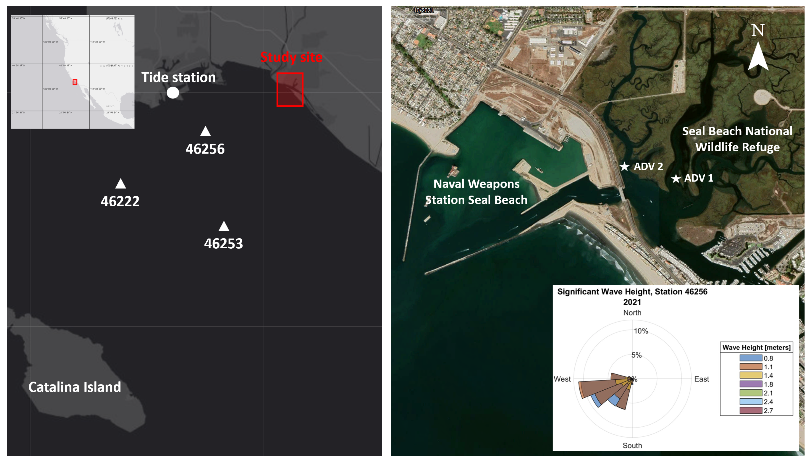
2.1. Study Area and Data Acquisition

Naval Weapons Station Seal Beach (NWSSB) is located in Orange County, California, at coordinates 33°43′30″ N and 118°04′51″ W. NWSSB primarily functions as a munitions storage and supply facility for the Navy, Coast Guard, and Marine Corps. The Seal Beach National Wildlife Refuge, shown in Figure 1, is within Naval Weapons Station Seal Beach and is a semi-intact saltwater marsh offering vital habitat for a range of species. Tides propagate through a stabilized navigation channel that leads to the refuge wetlands and a boat harbor. The open coast faces southwest. Dominant wave energy is from the northwest (Aleutian Low), west (Pineapple Express) and south [36]; see Figure 1. Catalina Island provides partial sheltering from southwestern swells.
In this study, two acoustic Doppler velocimeters (ADV) were utilized to collect data from the Seal Beach National Wildlife Refuge from 20 August 2020 16:00 to 4 October 2020 20:00. The harbor configuration was modified between 2020 and 2021, with modifications including a new pier and channel configuration seaward of the HW1 bridge. ADV 1 was redeployed from 23 April 2021 17:00 to 6 June 2021 16:00. The ADVs were mounted downward looking on a sawhorse frame secured to the bed on an intertidal mudflat. ADV 1 was deployed at the primary channel (Figure 1), recording 16-min bursts every hour at a sampling frequency of 8 Hz. The instrument’s blanking distance was 50 cm above the bed level. ADV 2 was deployed at a secondary channel (Figure 1), recording 16-min bursts every hour at a sampling frequency of 8 Hz. ADV 2 was deployed at a deeper location, allowing it to record a wider range of tidal water levels (Figure 2).

2.2. Data Preparation

The entire ADV 1 recordings dataset (observational periods of 2020 and 2021) was partitioned into 16-min blocks. Blocks that contained sporadic dry periods were excluded from the analysis, the forecasting of IG waves at that location being the ultimate goal of this work. For each block, the mean water depth (d) was calculated as the time-averaged value of the water depth (h). This led to a dataset consisting of 931 16-min blocks.
The primary flow direction at both ADV locations is along-channel. Thus, the computed horizontal velocities by principal axes analysis ( u ¯ and v ¯ ) represent the along-channel ( u ¯ ) and cross-channel ( v ¯ ) components of the velocity. Each time block velocity was computed as the time averages of the corresponding velocities in the along- and cross-channel directions (i.e., u, v). For example, at the ADV 1 location the principal axes reflect the surrounding bathymetry and the along-channel direction such that flood currents are in the northwest direction and ebb currents are in the southeast direction.
Meteo-marine observations, including atmospheric pressure, wind velocity magnitude, and direction, along with tidal water level data, were recorded by the NOAA 9410660 station located at the Long Beach harbor, Los Angeles (tidesandcurrents.noaa.gov). Offshore wave conditions were obtained from the NOAA offshore wave stations 46256 (Long Beach Channel, CA, 33°42′1″ N, 118°12′2″ W), 46253 (San Pedro South, CA, 33°34′33″ N, 118°10′53″ W) and 46222 (San Pedro, CA, 33°37′5″ N, 118°19′1″ W); see Figure 1, (www.ndbc.noaa.gov).

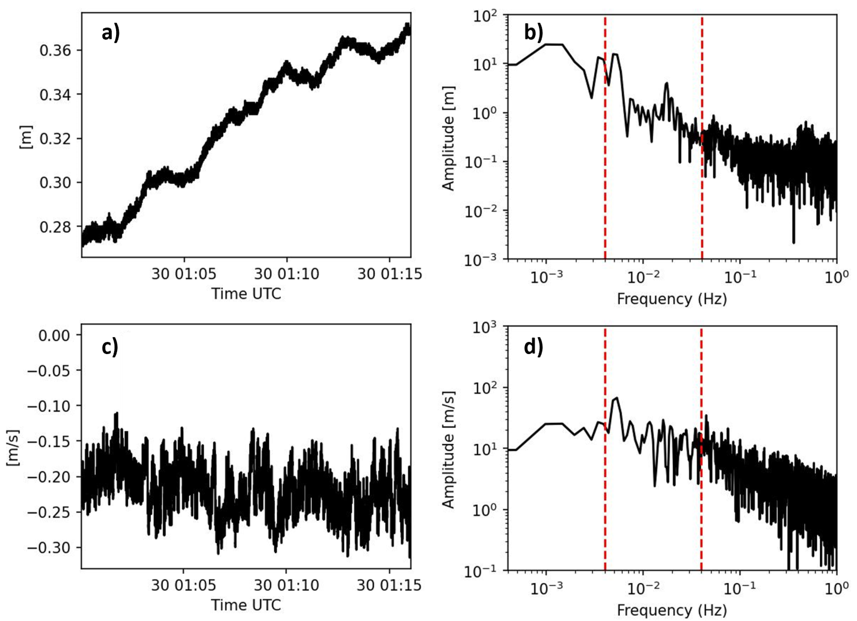
2.3. Signal Processing

A Fourier transform was applied to the observed water levels (OWL). The power spectrum of the recorded water level and flow velocity bursts show energy levels peaking within the IG band (Figure 3). Three sub-bands within the IG band were analyzed for their different frequency band behaviors and relationships with offshore wave parameters. The definition of the IG band varies slightly among authors (e.g., (30 s–5 min) Masselink et al. [37], (25 s–4 min) Herbers et al. [18]). In this study, the IG band is defined as 25 s to 5 min, consistent with Munk [8]. ADV data were band-pass filtered using a third-order Butterworth filter to remove frequencies higher and lower than the IG limits [3].
In this study, two estimators of estuary IG energy are considered and compared (Figure 4). The first estimator is the short-term energy ( S T E ) of the signals; this estimator is widely used in speech recognition methodologies to detect amplitude changes in digital signals [38], which are computed directly from the filtered signals by:
S T E = n = 1 N D ( n ) 2 ,
where N is the sample length of the signal and D ( n ) is the sampled points.
A common estimator found in the literature for IG energy is the significant wave height ( H s , I G ), computed as:
H s , I G = 4 m 0 ,
where m 0 is the variance of the filtered IG signal [19]. The two IG estimators within the estuary exhibit similar distributions, suggesting that they may be used interchangeably (Figure 4(a.1,a.2)).
A variance spectral density wave spectrum (S) was obtained using Welch’s method [39]. Using this spectrum, the orbital velocities ( v o r b ) associated with IG oscillations [3,40] can be calculated as follows:
v o r b = 2 f m a x f m i n ( S u + S v ) d f
where f m a x and f m i n are the IG band limits and S u and S v are the power spectra related to the horizontal components of the flow velocity.
The Pearson linear correlation coefficients (r) were computed to assess the degree of influence of the investigated variables on the IG energy within the estuary. The coefficients were calculated using the formula:
r = ( x ( i ) x ¯ ) ( y ( i ) y ¯ ) ( x ( i ) x ¯ ) 2 ( y ( i ) y ¯ ) 2
where x ( i ) and y ( i ) are the potentially correlated variables.

2.4. Machine Learning

This study aims to investigate the possibility of predicting the IG significant wave height at the ADV 1 location within the estuary by using offshore wave climate data (from NOAA buoys), along with coastal meteorological and tidal observations (from the Long Beach harbor station). The assumptions of multivariate regression analysis are normal distribution, linearity, and freedom from extreme values [41]. Non-linear relations have been found between offshore short-period wave parameters and IG levels [42]. Given the intricate relationships between the offshore wave conditions and the IG energy present within the estuary, traditional formulations may not adequately capture these complex correlations. Thus, ML algorithms have been selected as a suitable approach. Two ML algorithms are selected and compared: support vector machines (SVM) [43] and random forest classifier (RFC) [44]. Given the small size of the dataset used in this study, we opt for the use of shallow ML techniques. This decision is motivated by the potential risk of overfitting the data, which could lead to drops in performance [45]. Both algorithms can be used for both classification and regression tasks. The SVM algorithm determines a hyperplane that maximizes the margin between the closest point of each class and the hyperplane, using a convex cost function to reach the global minimum. In this study, a non-linear kernel (i.e., the radial basis function (RBF)) is selected to handle the non-linear nature of the process. RFC is an ensemble technique based on decision trees that can be used for both classification and regression tasks, such as support vector regressor (SVR) [46]. The RFC algorithm operates by dividing the dataset into smaller subsets and has been shown to be effective in a variety of contexts [47,48].
Feature vectors are utilized as input to the ML algorithms for estimating the magnitude of the IG oscillations. It should be noted that regularization (normalization) of the features is necessary before applying support vector regressor (SVR), due to significant differences in the order of magnitude between the feature values. However, regularization is not required for random forest classifier (RFC). The K-fold (10-fold) cross-validation technique [49,50] is applied in this study. To identify the optimal ML model, hyper-parameters grid search (5-fold) is applied to the training set. In K-fold validation methodology, the dataset is divided into k independent subsets of approximately equal size. One of these subsets is left out and will be utilised exclusively to test the model performance. The ML model is trained on k 1 of these subsets; this process is repeated k times, with each subset used exactly once as the validation data. For every fold, the model is trained with approximately 90% of the data and validated with the remaining independent 10%, leading to a performance metric.
Finally, the performance of the model is then averaged across all k iterations. The sum of squared errors ( S S E ) is selected as a metric for evaluating the applicability of the ML algorithms, which is calculated by:
S S E = i = 1 n ( y i f ( x i ) ) 2 ,
where n is the size of the test set, y i are the actual values in the test set, and f ( x i ) are the predictions made by the ML algorithms.
Additionally, the R-squared ( R 2 ) estimator, which represents the part of the variance for a dependent variable that is explained by the independent variables in a regression algorithm, is computed by:
R 2 = 1 S r e s / S t o t ,
where S r e s is the sum of squares of the residual errors and S t o t is the total sum of the errors.
In the context of training the ML algorithms, several characteristics related to the meteorological conditions and offshore wave climate were selected as features (Table 1). The 16-min blocks of data recorded each hour result in one IG significant wave height per hour, i.e., the input features are based on hourly average values. Additionally, the recorded hourly averaged tidal water levels at Long Beach harbor tide station and the meteorological conditions are used as features (i.e., wind magnitude and direction and atmospheric pressure).
IG waves are significantly influenced by incident swell direction [18]. Hence, the mean swell direction is considered a feature for training the ML algorithms. We investigated correlations among the variables T p , H s , and H s T p 2 , derived from data recorded by NOAA wave buoys, in relation to estuarine significant wave height. Similarly to Ardhuin et al. [51], the parameter H s T p 2 was included in the analysis due to the IG wavelength scaling with T 2 [42,52]. The H s T p 2 parameter exhibited the highest correlation coefficients (see Figure 5). Consequently, H s T p 2 was chosen as a feature for training the machine-learning algorithms. Additionally, features based on the lower frequency range of the wave spectrum recorded by the NOAA buoys (0.04–0.11 Hz) are incorporated into the dataset, as swell waves are considered to be the primary contributor to the generation of IG waves [12,18,53]. Note that alternative implementations of the parameter H s T p 2 (e.g., H s and T p separately as input features) are feasible and may yield different performances of the ML algorithms.
The features obtained from the lower portion of the frequency spectrum include the statistical measures of skewness and kurtosis, as well as the area beneath the energy spectrum curve. The kurtosis is calculated as:
K u r t o s i s = n = 1 N ( X n X ¯ ) 4 N σ 4 ,
where σ represents the standard deviation, N the total number of samples considered, and X ¯ is the average. The skewness is described as:
S k e w n e s s = n = 1 N ( X n X ¯ ) 3 N σ 3
Additionally, the frequency corresponding to the maximum point of spectral density ( F p , s w e l l ) recorded by the NOAA buoy is included as an ML training feature (Table 1).

3. Results

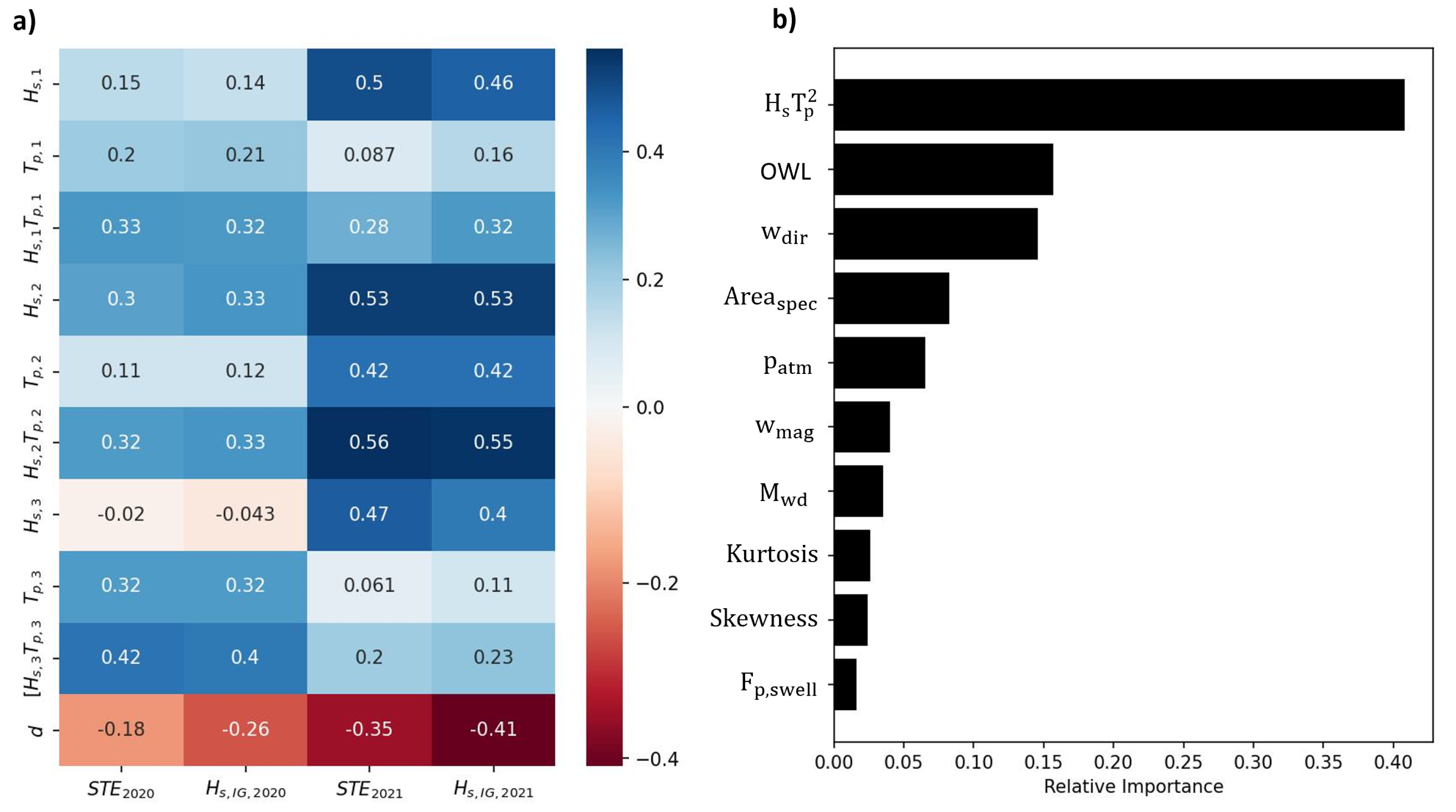
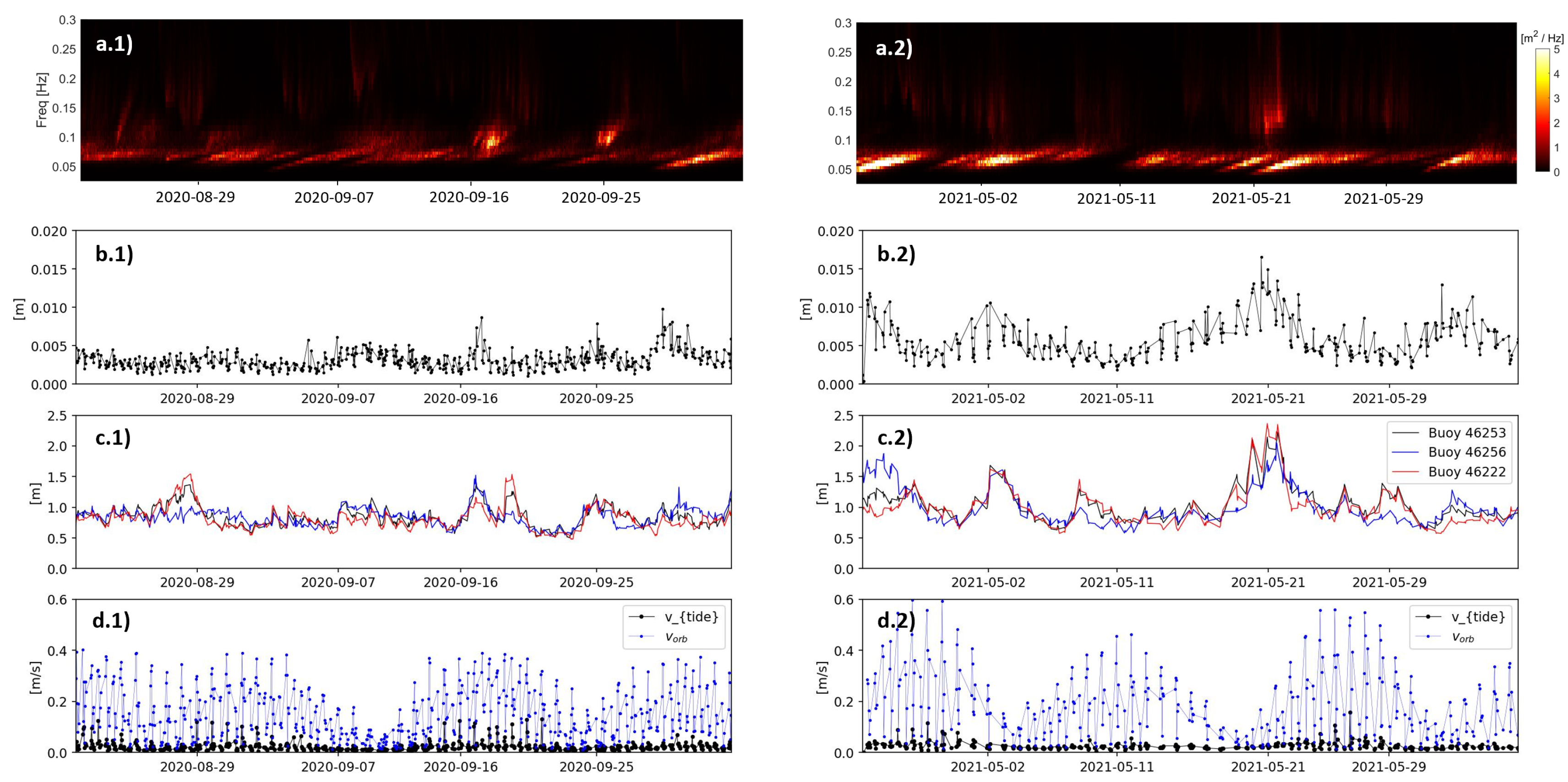
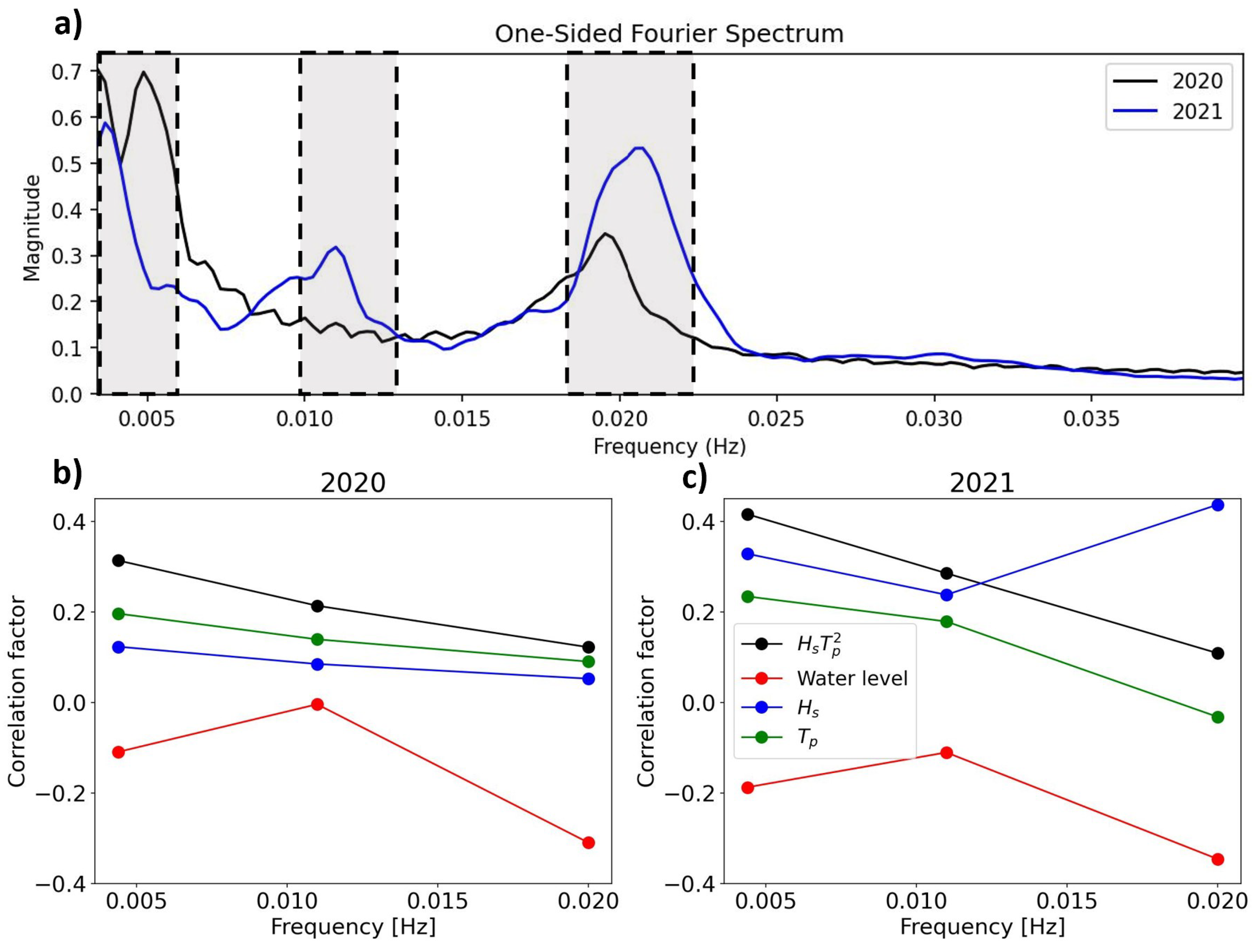
3.1. Infragravity Correlations and Orbital Velocities

IG significant wave heights inside the estuary were calculated and their correlation with the offshore wave climate recorded by the NOAA buoys. Water levels measured by tide gauges for both observational periods were established using Pearson linear correlation formula (Figure 6). The 2021 observational period exhibited stronger associated wave conditions compared to 2020. Accordingly, higher IG energy levels within the estuary were expected and observed in 2021 (Figure 6b).
The RFR algorithm allows the classification of the input features by importance scores based on the reduction in the criterion used to select split points, Gini impurity in this case (Figure 5). To estimate feature importance, the Gini gain is calculated, which is the amount of Gini impurity that was eliminated at each branch of the decision tree. H s T p 2 (offshore wave conditions), tidal levels, and wind direction are identified as the main features that can provide information forecasting future IG energy levels in the estuary.
Correlations between the IG levels ( S T E and H s , I G ) inside the estuary and the offshore wave conditions are dependent on the offshore instrument location. Notably, the correlations between the estuarine IG levels and the offshore wave conditions varied for the three considered buoys. Generally, the buoy situated nearest to the estuary mouth and in the shallowest water (buoy 46,256) shows the highest correlation with measured IG energy levels within the estuary (Figure 6(c.1,c.2) and Figure 5a). For example, the H s , I G correlation for buoy 46,256 is 0.33 and 0.53 in 2020 and 2021, respectively. This observation suggests that IG oscillations within the estuary are most related to the local (i.e. nearest) offshore wave conditions. Buoys located farther from the study site (∼33 km, buoy 46,222) exhibit moderate correlations with the IG measured within the estuary; however, these correlations increase as selected buoys closer to the study site are analyzed. This implies that estuarine IG oscillations may also be correlated with the wave climate at more distant locations (Figure 5a). The correlation coefficients calculated for the 2021 observational period were found to be higher compared to 2020, which can be attributed to a modification of the harbor configuration that provides entrance to the estuary. Negative correlations between IG oscillations and water levels were identified, suggesting that water levels are a relevant variable for the prediction of IG oscillations within the estuary. We also speculate that such correlations could be related to changes in wave reflections due to temporal variation in the beach slope during a tidal cycle [54]. Consistent with the literature, we observe that water levels are correlated with the IG wave energy present in the estuary [26,55] (Figure 5a). The features F p , s w e l l and the skewness and kurtosis of the swell part of the spectra are noted to exhibit low relative importance in the prediction of estuarine IG oscillations by the RFR algorithms (Figure 5b). Consequently, the removal of the mentioned input features may result in minimal performance variations.
The IG wave-generated orbital velocities, v o r b , were calculated as follows [40]:
v o r b = 2 f m i n f m a x S u + S v d f
where S u and S v are the horizontal velocity components spectra and ( f m i n , f m a x ) were set to the IG band limits (0.004–0.4) Hz. A variance spectral density wave spectrum, S, was calculated with the Welch’s method [39] using u and v as input for each block.
IG orbital velocities are known to have a significant impact on the suspended sediment in the water column and increase the sediment transport within the estuary [3,40]. The computed IG orbital velocities exhibit magnitudes that, in some events, exceed 20 % of the total tidal velocities, IG orbital velocity maxima can reach up to approximately 0.18 m/s (Figure 6(d.1,d.2)).
Tidal current impact on the IG energy transmission into the estuary was examined. The average observed IG energy corresponding to each recorded tidal level at ADV 2, which captured a broader range of tidal levels due to its deeper positioning, was computed and plotted against tidal water levels (Figure 7(b.1,b.2)). Lower tidal levels might facilitate IG propagation into the estuary, leading to higher IG energy levels (Figure 7(d.1,d.2)). Upon closer inspection of the spectra at low (lower than the mean low water level) and high (higher than the mean high water level) recorded tidal levels, a discernible shift in the highest frequency peaks and attenuation in the lowest two peaks were observed (Figure 7(d.1,d.2)). This suggests that higher tides may induce a frequency shift and attenuate IG energy. Additionally, the average spectra associated with ebbing and flooding stages are analyzed. Consistent with the literature (i.e., Mendes et al. [3], Williams and Stacey [19]), the data suggest that ebbing currents impede IG wave propagation inside the estuary due to their opposing velocity direction (Figure 7(c.1,c.2)).
To identify the most energetic wave frequencies within the IG band present inside the estuary during the recording period, the spectra obtained for each water level burst are added up and the maxima are identified. Three narrow frequency bands ((0.01–0.013) Hz, (0.018–0.023) Hz, and (0.0033–0.0054) Hz), which lie within the IG frequency band limits, were extracted from the recordings and correlated with the offshore wave conditions and water levels (Figure 8). The chosen frequency bands correspond with the three most energetic peaks in the data (Figure 8). The extracted lower frequency bands showed higher correlations with the offshore wave parameters than with the complete IG band, while the higher frequency bands had lower calculated correlations. Observations suggest different frequencies within the IG band behave differently to changing offshore wave conditions and tidal water levels. IG waves in close proximity to 0.02 Hz demonstrate the strongest negative correlation (< 0.3 ) with water levels when compared to the other frequencies investigated. Additionally, although average frequency spectra of the observed water levels show similar behavior for the 2020 and 2021 observational periods, differences may be associated with the channel realignment, suggesting channel morphology is impacting IG propagation into the estuary.

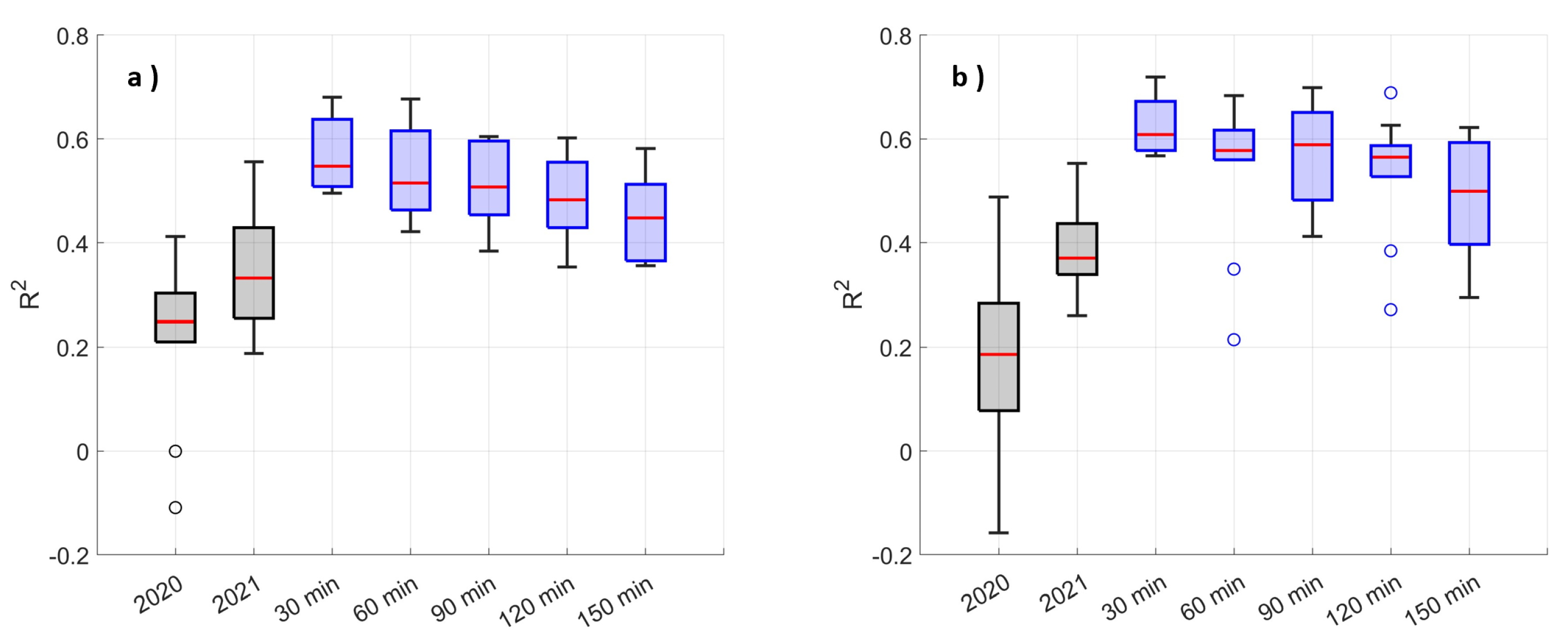
3.2. Infragravity Predictions

IG-induced seiching has been shown to substantially affect ports and harbor operations (e.g., González-Marco et al. [56], Cuomo and Guza [57], Okihiro et al. [58]). In this section, we present a novel approach, where IG oscillations inside the Seal Beach National Wildlife Refuge estuary are forecast half an hour ahead. This approach is based on the fact that relevant correlations between offshore wave conditions, water levels, and estuarine IG energy have been found. The features extracted from the offshore NOAA wave buoy records are chosen half an hour ahead of the estimated IG wave heights due to cross-correlation analysis computed between the IG significant wave height time series and the offshore H s T p 2 time series recorded by NOAA buoy 46,256, which showed a 0.51 h lag difference. For this analysis, only the most energetic events were selected, see the area highlighted in yellow in Figure 7a.
The presented ML algorithms are implemented on the generated dataset, and the averaged 10-fold outcomes are depicted in Table 2 and Figure 9. The random forest regression (RFR) algorithm attains the highest prediction accuracy, where the IG significant wave height inside the estuary is predicted with R 2 > 0.6 and low RMSE, while the SVR algorithm underpredicts H s , I G values (Figure 9, Table 2).
The ability of the RFR and SVM algorithms to predict IG along with decomposing the variable H s T p 2 into two input variables, H s and T p has been assessed. This approach resulted in regression performances of R 2 = 0.614 and MSE = 1.92 × 10 −6 m 2 for RFR and R 2 = 0.556 and MSE = 2.22 × 10 6 m 2 for SVM. Both examined ML algorithms yielded lower performance metrics when the variable H s T p 2 was divided into two independent variables ( H s and T p ) serving as input features.
It is noteworthy to mention that incorporating meteorological parameters, specifically atmospheric pressure and wind magnitude, resulted in a ∼5% increase in the efficacy of the ML algorithms. We speculate that variations in atmospheric pressure and local winds may be responsible for generating some of the IG oscillations inside the studied estuary.
Finally, the efficacy of the presented methodology to forecast IG oscillations with the use of varying prediction time windows is tested. It can be observed (Figure 10) that predictive accuracy diminishes with the extension of forecast time. The prediction ability is higher when exclusively utilizing the observational data from 2021, which in combination with the higher correlations observed for the same observational period between IG oscillations within the estuary and offshore variables potentially indicates that modifications to harbor configurations contribute to an increase in the potential for the IG waves to propagate into the estuary.

4. Conclusions

This work investigates IG oscillation forecasting in a shallow, low inflow estuary. The study employs a combination of water level and flow velocity oscillations measured by two ADVs inside the estuary. ML algorithms are used to predict IG oscillations.
This work involved the examination of wave climate data recorded by three NOAA buoys located at varying distances from the estuary mouth. The analysis reveals moderate correlations (>0.5) between estuarine IG levels and offshore wave conditions, indicating that some of the IG energy in the estuary originates from the offshore swell. The buoy located nearest to the estuary mouth exhibited the highest correlations. Consequently, it was chosen as the optimal location for training machine-learning (ML) algorithms, which had half an hour lag to the measured estuarine IG levels, giving that as the forecast time window. We speculate that the location of the buoy is of high importance, with closer locations potentially leading to higher prediction accuracy but shorter forecast time windows. The offshore wave parameter weighting wave period, H s T p 2 , shows the highest correlation with estuarine IG oscillations. As found in other estuaries, flood tides are the most energetic while ebb currents block a portion of IG propagation into the estuary.
Orbital velocities related to IG reach up to 20% of total tidal velocities in this system, indicating that IG orbital motions may be important for sediment transport due to their significant magnitudes. This percentage is less than in other shallower estuarine systems, likely due to instrument site distance upstream and a deeper and wider overall estuary. The most energetic frequencies within the IG frequency band were analyzed, and it was observed that the different frequencies exhibit different correlations with offshore wave characteristics and tidal water levels, with lower frequencies being more correlated to the offshore swell, whereas higher frequencies are less correlated to offshore wave parameters, suggesting that they could be generated more locally. Tidal water levels are found to be negatively correlated with IG motions within the estuary, indicating that some of the IG energy that comes from offshore could be released by wave breaking in front of the harbor.
This study also presents a novel method of forecasting IG oscillations thirty minutes in advance within a small low-inflow estuary based on publicly available meteo-marine observations. However, due to the small dataset size, this is a proof of concept, and it is speculated that the inclusion of more data in the ML training could increase the accuracy of the presented methodology and reduce model uncertainties. Note that the particular algorithms produced here are specific to SBNWR. To apply the same methodology to alternative sites (other LIEs, but also other harbors and embayments), IG observations at the specific location would be required. This paper presents a guideline for the implementation of this technology, such as the potential location of the required instrumentation and significance of specific variables, including water levels, offshore wave conditions, and meteorological parameters.

Author Contributions

Conceptualization, B.G., T.G., and S.N.G.; methodology, B.G., T.G., and S.N.G.; software, B.G.; formal analysis, B.G., T.G., and S.N.G.; investigation, B.G., T.G., and S.N.G.; resources, B.G., T.G., and S.N.G.; writing—original draft preparation, B.G., T.G., and S.N.G.; writing—review and editing, B.G., T.G., and S.N.G.; visualization, B.G.; project administration, B.G., T.G., and S.N.G.; funding acquisition, T.G. and S.N.G. All authors have read and agreed to the published version of the manuscript.

Funding

This study was funded by the US Navy on contract N624473-19-0016 and California Parks and Recreation, Division of Boating and Waterways contacts C1670006 and C22820007.

Institutional Review Board Statement

Not applicable.

Informed Consent Statement

Not applicable.

Data Availability Statement

The data supporting the reported results can be obtained from the corresponding author.

Acknowledgments

We would like to acknowledge Jess Curran, Megan Hanna, and Bob Schallmann for helping arrange estuary access. Thank you to Brian Woodward, Kent Smith, Rob Grenzeback, Lucien Parry, Shane Finnerty, Carson Black, Chloe Van Grootheest, Christine Whitcraft, Burson Tang, Joseph Lucey, MP Delisle, and Margit Maple, who participated in the field work and observations that made this manuscript possible.

Conflicts of Interest

The authors declare no conflicts of interest.

Abbreviations

The following abbreviations are used in this manuscript:
NOAANational Oceanic and Atmospheric Administration
CDIPCoastal Data Information Program

References

  1. Taherkhani, M.; Vitousek, S.; Walter, R.K.; O’Leary, J.; Khodadoust, A.P. Flushing time variability in a short, low-inflow estuary. Estuar. Coast. Shelf Sci. 2023, 284, 108277. [Google Scholar] [CrossRef]
  2. Zedler, J.B.; Kercher, S. Wetland resources: Status, trends, ecosystem services, and restorability. Annu. Rev. Environ. Resour. 2005, 30, 39–74. [Google Scholar] [CrossRef]
  3. Mendes, D.; Fortunato, A.B.; Bertin, X.; Martins, K.; Lavaud, L.; Silva, A.N.; Pires-Silva, A.A.; Coulombier, T.; Pinto, J.P. Importance of infragravity waves in a wave-dominated inlet under storm conditions. Cont. Shelf Res. 2020, 192, 104026. [Google Scholar] [CrossRef]
  4. Harvey, M.E.; Giddings, S.N.; Pawlak, G.; Crooks, J.A. Hydrodynamic Variability of an Intermittently Closed Estuary over Interannual, Seasonal, Fortnightly, and Tidal Timescales. Estuaries Coasts 2022, 46, 84–108. [Google Scholar] [CrossRef]
  5. Largier, J.L. Recognizing Low-Inflow Estuaries as a Common Estuary Paradigm. Estuaries Coasts 2023, 46, 1949–1970. [Google Scholar] [CrossRef]
  6. McSweeney, S.L.; Stout, J.C.; Kennedy, D.M. Variability in infragravity wave processes during estuary artificial entrance openings. Earth Surf. Process. Landforms 2020, 45, 3414–3428. [Google Scholar] [CrossRef]
  7. Duong, T.M.; Ranasinghe, R.; Walstra, D.; Roelvink, D. Assessing climate change impacts on the stability of small tidal inlet systems: Why and how? Earth-Sci. Rev. 2016, 154, 369–380. [Google Scholar] [CrossRef]
  8. Munk, W. Surf beats. EOS Trans. Am. Geophys. Union 1949, 30, 849–854. [Google Scholar]
  9. Aagaard, T.; Greenwood, B.; Hughes, M. Sediment transport on dissipative, intermediate and reflective beaches. Earth-Sci. Rev. 2013, 124, 32–50. [Google Scholar] [CrossRef]
  10. Costas, R.; Carro, H.; Figuero, A.; Peña, E.; Sande, J. A Decision-Making Tool for Port Operations Based on Downtime Risk and Met-Ocean Conditions including Infragravity Wave Forecast. J. Mar. Sci. Eng. 2023, 11, 536. [Google Scholar] [CrossRef]
  11. Uncles, R.; Stephens, J.; Harris, C. Infragravity currents in a small ría: Estuary-amplified coastal edge waves? Estuar. Coast. Shelf Sci. 2014, 150, 242–251. [Google Scholar] [CrossRef]
  12. Okihiro, M.; Guza, R. Observations of seiche forcing and amplification in three small harbors. J. Waterw. Port Coastal Ocean Eng. 1996, 122, 232–238. [Google Scholar] [CrossRef]
  13. Rabinovich, A.B. Seiches and harbor oscillations. In Handbook of Coastal and Ocean Engineering; World Scientific: Singapore, 2010; pp. 193–236. [Google Scholar]
  14. López, M.; Iglesias, G. Artificial intelligence for estimating infragravity energy in a harbour. Ocean Eng. 2013, 57, 56–63. [Google Scholar] [CrossRef]
  15. Tucker, M. Surf beats: Sea waves of 1 to 5 min. period. Proc. R. Soc. London. Ser. A. Math. Phys. Sci. 1950, 202, 565–573. [Google Scholar]
  16. Bowers, E. Harbour resonance due to set-down beneath wave groups. J. Fluid Mech. 1977, 79, 71–92. [Google Scholar] [CrossRef]
  17. Elgar, S.; Herbers, T.; Okihiro, M.; Oltman-Shay, J.; Guza, R. Observations of infragravity waves. J. Geophys. Res. Ocean. 1992, 97, 15573–15577. [Google Scholar] [CrossRef]
  18. Herbers, T.; Elgar, S.; Guza, R. Generation and propagation of infragravity waves. J. Geophys. Res. Ocean. 1995, 100, 24863–24872. [Google Scholar] [CrossRef]
  19. Williams, M.E.; Stacey, M.T. Tidally discontinuous ocean forcing in bar-built estuaries: The interaction of tides, infragravity motions, and frictional control. J. Geophys. Res. Ocean. 2016, 121, 571–585. [Google Scholar] [CrossRef]
  20. Bertin, X.; de Bakker, A.; Van Dongeren, A.; Coco, G.; André, G.; Ardhuin, F.; Bonneton, P.; Bouchette, F.; Castelle, B.; Crawford, W.C.; et al. Infragravity waves: From driving mechanisms to impacts. Earth-Sci. Rev. 2018, 177, 774–799. [Google Scholar] [CrossRef]
  21. Baldock, T.; Huntley, D.; Bird, P.; O’hare, T.; Bullock, G. Breakpoint generated surf beat induced by bichromatic wave groups. Coast. Eng. 2000, 39, 213–242. [Google Scholar] [CrossRef]
  22. Stiassnie, M.; Drimer, N. Prediction of long forcing waves for harbor agitation studies. J. Waterw. Port Coastal, Ocean Eng. 2006, 132, 166–171. [Google Scholar] [CrossRef]
  23. Bellotti, G. Transient response of harbours to long waves under resonance conditions. Coast. Eng. 2007, 54, 680–693. [Google Scholar] [CrossRef]
  24. Melito, I.; Cuomo, G.; Bellotti, G.; Franco, L. Field measurements of harbour resonance at Marina di Carrara. In Coastal Engineering 2006: (In 5 Volumes); World Scientific: Singapore, 2007; pp. 1280–1292. [Google Scholar]
  25. Bertin, X.; Olabarrieta, M. Relevance of infragravity waves in a wave-dominated inlet. J. Geophys. Res. Ocean. 2016, 121, 5418–5435. [Google Scholar] [CrossRef]
  26. Bowers, E. Low frequency waves in intermediate water depths. In Coastal Engineering 1992; HR Wallingford: Oxfordshire, UK, 1992; pp. 832–845. [Google Scholar]
  27. Melito, L.; Postacchini, M.; Sheremet, A.; Calantoni, J.; Zitti, G.; Darvini, G.; Brocchini, M. Wave-current interactions and infragravity wave propagation at a microtidal inlet. Proceedings 2018, 2, 628. [Google Scholar] [CrossRef]
  28. Wheeler, D.C.; Giddings, S.N. Measuring Turbulent Dissipation with Acoustic Doppler Velocimeters in the Presence of Large, Intermittent, Infragravity Frequency Bores. J. Atmos. Ocean. Technol. 2023, 40, 285–304. [Google Scholar] [CrossRef]
  29. Bertin, X.; Mendes, D.; Martins, K.; Fortunato, A.B.; Lavaud, L. The closure of a shallow tidal inlet promoted by infragravity waves. Geophys. Res. Lett. 2019, 46, 6804–6810. [Google Scholar] [CrossRef]
  30. Bromirski, P. Climate-Induced Decadal Ocean Wave Height Variability From Microseisms: 1931–2021. J. Geophys. Res. Ocean. 2023, 128, e2023JC019722. [Google Scholar] [CrossRef]
  31. Oh, J.; Suh, K.D. Real-time forecasting of wave heights using EOF–wavelet–neural network hybrid model. Ocean Eng. 2018, 150, 48–59. [Google Scholar] [CrossRef]
  32. Granata, F.; Di Nunno, F. Artificial Intelligence models for prediction of the tide level in Venice. Stoch. Environ. Res. Risk Assess. 2021, 35, 2537–2548. [Google Scholar] [CrossRef]
  33. Williams, B. Predicting infragravity wave height in harbours using artificial intelligence. In Proceedings of the Australasian Coasts and Ports 2019 Conference: Future directions from 40 [degrees] S and beyond, Hobart, Australia, 10–13 September 2019; Engineers Australia Hobart: Hobart, TAS, Australia, 2019; pp. 1226–1232. [Google Scholar]
  34. Zheng, Z.; Ma, X.; Ma, Y.; Dong, G. Wave estimation within a port using a fully nonlinear Boussinesq wave model and artificial neural networks. Ocean Eng. 2020, 216, 108073. [Google Scholar] [CrossRef]
  35. Zheng, Z.; Ma, X.; Huang, X.; Ma, Y.; Dong, G. Wave forecasting within a port using WAVEWATCH III and artificial neural networks. Ocean Eng. 2022, 255, 111475. [Google Scholar] [CrossRef]
  36. Adams, P.N.; Inman, D.L.; Graham, N.E. Southern California deep-water wave climate: Characterization and application to coastal processes. J. Coast. Res. 2008, 24, 1022–1035. [Google Scholar] [CrossRef]
  37. Masselink, G.; Tuck, M.; McCall, R.; van Dongeren, A.; Ford, M.; Kench, P. Physical and numerical modeling of infragravity wave generation and transformation on coral reef platforms. J. Geophys. Res. Ocean. 2019, 124, 1410–1433. [Google Scholar] [CrossRef]
  38. Greenwood, M.; Kinghorn, A. SUVing: Automatic Silence/Unvoiced/Voiced Classification of Speech; Undergraduate Coursework, Department of Computer Science, University of Sheffield: Sheffield, UK, 1999; Volume 4. [Google Scholar]
  39. Welch, P. The use of fast Fourier transform for the estimation of power spectra: A method based on time averaging over short, modified periodograms. IEEE Trans. Audio Electroacoust. 1967, 15, 70–73. [Google Scholar] [CrossRef]
  40. Wiberg, P.L.; Sherwood, C.R. Calculating wave-generated bottom orbital velocities from surface-wave parameters. Comput. Geosci. 2008, 34, 1243–1262. [Google Scholar] [CrossRef]
  41. Alexopoulos, E.C. Introduction to multivariate regression analysis. Hippokratia 2010, 14, 23. [Google Scholar] [PubMed]
  42. Oh, J.; Suh, K.D.; Oh, S.H.; Jeong, W.M. Estimation of infragravity waves inside Pohang New Port. J. Coast. Res. 2016, 432–436. [Google Scholar] [CrossRef]
  43. Boser, B.E.; Guyon, I.M.; Vapnik, V.N. A training algorithm for optimal margin classifiers. In Proceedings of the Fifth Annual Workshop on Computational Learning Theory, Pittsburgh, PA, USA, 27–29 July 1992; pp. 144–152. [Google Scholar]
  44. Ho, T.K. Random decision forests. In Proceedings of the 3rd International Conference on Document Analysis and Recognition, Montreal, QC, Canada, 14–16 August 1995; Volume 1, pp. 278–282. [Google Scholar]
  45. Pasupa, K.; Sunhem, W. A comparison between shallow and deep architecture classifiers on small dataset. In Proceedings of the 2016 8th International Conference on Information Technology and Electrical Engineering (ICITEE), Yogyakarta, Indonesia, 5–6 October 2016; pp. 1–6. [Google Scholar]
  46. Breiman, L. Random forests. Mach. Learn. 2001, 45, 5–32. [Google Scholar] [CrossRef]
  47. Breiman, L. Classification and Regression Trees; Routledge: London, UK, 2017. [Google Scholar]
  48. Gomez, B.; Kadri, U. Earthquake source characterization by machine learning algorithms applied to acoustic signals. Sci. Rep. 2021, 11, 23062. [Google Scholar] [CrossRef]
  49. Stone, M. Cross-validatory choice and assessment of statistical predictions. J. R. Stat. Soc. Ser. B (Methodol.) 1974, 36, 111–133. [Google Scholar] [CrossRef]
  50. Stone, M. An asymptotic equivalence of choice of model by cross-validation and Akaike’s criterion. J. R. Stat. Soc. Ser. B (Methodol.) 1977, 39, 44–47. [Google Scholar] [CrossRef]
  51. Ardhuin, F.; Rawat, A.; Aucan, J. A numerical model for free infragravity waves: Definition and validation at regional and global scales. Ocean Model. 2014, 77, 20–32. [Google Scholar] [CrossRef]
  52. Nwogu, O.; Demirbilek, Z. Infragravity wave motions and runup over shallow fringing reefs. J. Waterw. Port Coastal Ocean Eng. 2010, 136, 295–305. [Google Scholar] [CrossRef]
  53. Harkins, G.S.; Briggs, M.J. Resonant forcing of harbors by infragravity waves. In Coastal Engineering 1994; Alexander Bell Drive: Reston, VA, USA, 1995; pp. 806–820. [Google Scholar]
  54. Rijnsdorp, D.P.; Reniers, A.J.; Zijlema, M. Free infragravity waves in the North Sea. J. Geophys. Res. Ocean. 2021, 126, e2021JC017368. [Google Scholar] [CrossRef]
  55. Su, S.F.; Ma, G.; Hsu, T.W. Boussinesq modeling of spatial variability of infragravity waves on fringing reefs. Ocean Eng. 2015, 101, 78–92. [Google Scholar] [CrossRef]
  56. González-Marco, D.; Sierra, J.P.; de Ybarra, O.F.; Sánchez-Arcilla, A. Implications of long waves in harbor management: The Gijón port case study. Ocean Coast. Manag. 2008, 51, 180–201. [Google Scholar] [CrossRef]
  57. Cuomo, G.; Guza, R. Infragravity seiches in a small harbor. J. Waterw. Port Coastal Ocean Eng. 2017, 143, 04017032. [Google Scholar] [CrossRef]
  58. Okihiro, M.; Guza, R.; Seymour, R. Excitation of seiche observed in a small harbor. J. Geophys. Res. Ocean. 1993, 98, 18201–18211. [Google Scholar] [CrossRef]
Figure 1. (Left): Locations for the study area, analyzed NOAA tide gauge (circle) and wave stations (triangles). (Right): Study area and ADV locations within the Seal beach estuary. On the bottom right corner are wave heights for station 46253 during 2021 (https://www.ndbc.noaa.gov/, accessed on 12 March 2024). Maps extracted from https://earthexplorer.usgs.gov/, accessed on 12 March 2024.
Jmse 12 00672 g001
Figure 2. Recorded water levels by ADV 1 and ADV2.
Jmse 12 00672 g002
Figure 3. (a) Water level time series for one 16-min ADV burst and (b) its associated frequency spectrum. (c) Principal axes flow velocity time series for the same 16-min ADV burst and (d) the associated frequency spectrum. The vertical dashed red lines represent the IG frequency band limits.
Jmse 12 00672 g003
Figure 4. (a.1) Normalized IG significant wave height ( H s , I G ) and IG S T E temporal distribution for the analyzed water level ADV recordings at ADV 1 in 2020 and (a.2) 2021. (b.1) Significant wave height and peak period from the offshore nearest buoy, 46,256 in 2020 and (b.2) 2021. (c.1) Mean wave direction recorded by the buoy 46,256 in 2020 and (c.2) 2021. (d.1) Mean tidal water levels over each burst at ADV 1 in 2020 and (d.2) 2021. (e.1) Wind speed magnitude and direction in 2020 and (e.2) 2021. (f.1) Atmospheric pressure in 2020 and (f.2) 2021.
Jmse 12 00672 g004
Figure 5. (a) Correlation coefficients for the 2020 and 2021 ADV deployments. H s T p 2 , where H s and T p are the significant wave height and peak period for the considered NOAA wave buoys (subindices: 1–46,253, 2–46,256 and 3–46,222); d is the hourly tidal water level at Long Beach Harbor tide station. For all the obtained correlations, the obtained P value lies below 0.001. (b) RFR feature importance, Table 1.
Jmse 12 00672 g005
Figure 6. (a.1) Spectrogram associated with the CDIP buoy 46,256 during the observational periods of 2020 and (a.2) 2021. (b.1) Calculated estuarine IG significant wave height at ADV 1 during the 2020 observational period and (b.2) during the 2021 observational period. (c.1) Offshore significant wave height for the three considered NOAA buoy stations during the 2020 observational period and (c.2) during the 2021 observational period. (d.1) Tidal and orbital velocities recorded by ADV 1 during the 2020 observational period and (d.2) during the 2021 observational period.
Jmse 12 00672 g006
Figure 7. (a.1) Estuarine IG spectral energy for the observational period of 2020. (a.2) Total IG energy per burst from ADV 1. (b) Average energy per burst related to the tidal water level for both studied ADVs during the observational period of 2020. (c) Average frequency energy spectrum for ebbing and flooding stages at ADV 2. (d) Average frequency energy spectrum for the 20% highest and 20% lowest observed water levels for ADV 2.
Jmse 12 00672 g007
Figure 8. (a) Average frequency spectrum for the all the 2020 and 2021 analyzed recordings at ADV 1. The extracted IG sub-bands are highlighted in gray. (b) Calculated Pearson linear correlation coefficients between the S T E of different IG wave sub-bands and different variables, including offshore wave conditions and water levels for the recordings during 2020 and (c) 2021.
Jmse 12 00672 g008
Figure 9. IG significant wave height predicted values by the RFR and SVR algorithms against the actual values. The line in red represents the best fit.
Jmse 12 00672 g009
Figure 10. (a) SVR and (b) RFR algorithms applied first to a dataset constructed with the 2020 and 2021 observational periods in grey and to a dataset composed by both observational periods together with different prediction time windows. The circles represent outliers.
Jmse 12 00672 g010
Table 1. Features utilized as input of the ML algorithm. A r e a s p e c stands for the area under the wave frequency energy spectrum associated with the wave buoy recordings and M w d is the mean wave direction.
Buoy 46,256Tide StationMet. Station
H s T p 2 (ms2)OWL (m) p a t m (Pa)
M w d (Deg) w m a g (m/s)
A r e a s p e c w d i r (Deg)
F p , s w e l l (Hz)
K u r t o s i s
S k e w n e s s
Table 2. Final ML IG oscillation regression results after the application of hyperparameter grid search and k-fold technique. The features are listed in Table 1.
R 2 MSE (m2)
SVR0.5752.094 × 10 6
RFR0.6431.864 × 10 6
Disclaimer/Publisher’s Note: The statements, opinions and data contained in all publications are solely those of the individual author(s) and contributor(s) and not of MDPI and/or the editor(s). MDPI and/or the editor(s) disclaim responsibility for any injury to people or property resulting from any ideas, methods, instructions or products referred to in the content.

