Ocean-Mixer: A Deep Learning Approach for Multi-Step Prediction of Ocean Remote Sensing Data

Abstract

The development of intelligent oceans requires exploration and an understanding of the various characteristics of the oceans. The emerging Internet of Underwater Things (IoUT) is an extension of the Internet of Things (IoT) to underwater environments, and the ability of IoUT to be combined with deep learning technologies is a powerful technology for realizing intelligent oceans. The underwater acoustic (UWA) communication network is essential to IoUT. The thermocline with drastic temperature and density variations can significantly limit the connectivity and communication performance between IoUT nodes. To more accurately capture the complexity and variability of ocean remote sensing data, we first sample and analyze ocean remote sensing datasets and provide sufficient evidence to validate the temporal redundancy properties of the data. We propose an innovative deep learning approach called Ocean-Mixer. This approach consists of three modules: an embedding module, a mixer module, and a prediction module. The embedding module first processes the location and attribute information of the ocean water and then passes it to the subsequent modules. In the mixing module, we apply a temporal decomposition strategy to eliminate redundant information and capture temporal and channel features through a self-attention mechanism and a multilayer perceptron (MLP). The prediction module ultimately discerns and integrates the temporal and channel relationships and interactions among various ocean features, ensuring precise forecasting. Numerous experiments on ocean temperature and salinity datasets show that Mixer-Ocean performs well in improving the accuracy of time series prediction. Mixer-Ocean is designed to support multi-step prediction and capture the changes in the ocean environment over a long period, thus facilitating efficient management and timely decision-making for innovative ocean-oriented applications, which has far-reaching significance for developing and conserving marine resources.

1. Introduction

The Internet of Underwater Things (IoUT) aims to create an interconnected network of underwater systems that facilitates real-time monitoring and data transfer within marine ecosystems. Developing a comprehensive oceanic wireless 3D observation grid enables extensive surveillance of the marine environment but also plays a pivotal role in disaster preparedness, resource exploration, and national defense. Challenges arise due to the distinct nature of aquatic and aerial communication mediums and the adverse conditions prevalent in marine settings [1]. These challenges manifest as increased complexity in the communication channels spanning air and sea, as well as diminished efficiency in the data transmission capabilities of underwater networks.

Underwater Acoustic Communication (UAC) emerges as a pivotal technology within underwater wireless communication, offering a means to transmit data across substantial distances. It is capable of facilitating transmission over several kilometers at rates of hundreds of bits per second (bps) and across hundreds of meters at tens of kilobits per second (kbps) [2]. This capability establishes it as the preeminent communication technology utilized in underwater wireless sensor networks. Despite its efficacy, the marine environment introduces considerable temporal and spatial variability, marked by intricate and mutable periodic variations. Such dynamics engender pronounced spatio-temporal uncertainty, which presents substantial challenges to effective communication in these aquatic realms.

In underwater settings, various factors, including currents, temperature shifts, and salinity changes, can adversely affect signal transmission, potentially leading to significant attenuation and distortion. The oceanographic characteristics’ distribution is pivotal in dictating the attenuation, reflection, refraction, and scattering of acoustic waves. This interaction results in the creation of complex convergence and shadow zones within the IoUT [3,4]. The elaborate distribution of these zones is critical in determining the connectivity and communication performance among IoUT nodes. Moreover, it significantly influences the network topology, thereby impacting the reliability and stability of communications. This multifaceted interplay underscores the challenges and necessitates a nuanced understanding of the marine environment to enhance and innovate underwater wireless communications.

The oceanic thermocline, located between the surface and deeper layers of the ocean, is a layer of water whose temperature decreases significantly with depth. The depth and thickness of the thermocline varies according to geographic location, season, and climatic conditions. The thermocline is particularly pronounced in temperate and tropical waters [5]. Within the thermocline, the temperature drop is very rapid and can drop dramatically by tens of degrees over a vertical distance of a few tens of meters. This rapid temperature change significantly affects the speed of sound, causing the speed of sound waves to change as they pass through the thermocline. If the angle of incidence and temperature difference for sound wave propagation reaches certain conditions, the sound wave will also undergo a total reflection phenomenon [6]. The total reflection phenomenon may lead to limited connectivity of the hydroacoustic network. It also affects the communication between different nodes in the IoUT. Hence, the precise forecasting of crucial oceanic characteristics is imperative for formulating routing strategies in underwater acoustic networks.

In the oceanic thermocline, key parameters such as temperature, salinity, and density vary significantly depending on ocean depth, geographic coordinates, and time factors. In a dynamic ocean environment, these variations pose challenges for sensor deployment and network optimization and have significant implications for achieving effective data transmission and communication maintenance. While providing routing and media access control strategies for designing underwater network topology nodes, current prediction techniques still fail to meet the demand for longer-term and more accurate predictions for underwater communication systems. Specific challenges in the current prediction task include the following: (1) Oceanographic features display seasonal and cyclical variations. Long-term changes and trends in the ocean, such as global climate-induced shifts in sea temperature and ocean acidification, can impact the nature of the thermocline. Only multi-step temporal forecasting can trace the evolution of thermocline characteristics over extended time scales. (2) The process of collecting ocean data involves significant data redundancy. Temporal forecasting tasks in such intricate marine environments require extensive data collection and analysis. Insufficient or excessive data can both negatively impact the accuracy of thermocline predictions, thereby compromising the reliability of the final forecasting outcomes.

Our research objective is to leverage the historical states and patterns of the ocean to conduct multi-step, high-accuracy investigations into the temporal dynamics of the thermocline. Current methodologies for temporal forecasting predominantly encompass numerical techniques grounded in mathematical or statistical principles, as well as models derived from deep learning paradigms [7]. Within this spectrum, the numerical approaches relying on mathematical or statistical foundations typically employ polynomials, differential equations, and other mathematical constructs to approximate the patterns of ocean temperature variations [8]. Although these methods are straightforward to implement and facilitate rapid prediction generation, they often fail to accurately represent the ocean’s inherently nonlinear characteristics, leading to suboptimal model fittings.

In oceanographic research, the application of deep learning methodologies has gained significant traction in recent years, particularly in analyzing temporal characteristics of marine environments. This transition from rudimentary neural network architectures to more sophisticated deep learning frameworks has proven efficacious in accurately modeling ocean temperature variations’ intricate, nonlinear dynamics. Notably, convolutional neural networks (CNNs) exhibited remarkable proficiency in abstracting spatial features, a pivotal capability for predicting future states, as elucidated in [9]. Similarly, recurrent neural networks (RNNs) were adeptly employed for deciphering temporal dependencies in traffic speed prediction at discrete locations, drawing upon historical traffic data series, as expounded in [10]. Despite these advancements, it remains a challenge for a singular deep learning model to comprehensively assimilate the nuanced characteristics inherent in a diverse dataset, often resulting in an inability to concurrently address both spatial and temporal correlations effectively.

To better understand temporal and channel characteristics, the researchers developed an approach integrating feature vectors, encapsulating spatial dependencies, into recurrent neural network (RNN) sequences [11]. This integration aims to learn all spatio-temporal dependencies synergistically. Furthermore, Qin et al. [12] introduced a predictive model for red tide disasters, amalgamating the autoregressive integrated moving average (ARIMA) model with Deep Belief Networks (DBNs). This innovative model is employed to meticulously analyze the temporal correlations and spatial heterogeneity inherent among factors sensitive to red tides.

While existing methodologies demonstrate remarkable efficacy in concurrent spatio-temporal forecasting, their primary utility is confined to two-dimensional terrestrial landscapes, rendering them inadequate for the intricacies of three-dimensional marine environments characterized by latitude, longitude, and depth dimensions. As elaborated in [13], the proposed multilayer ConvLSTM (M-convLSTM) framework aims to prognostify internal oceanic temperatures. Nonetheless, the challenge of effectively parsing interdependencies within expansive and intricate datasets persists. Song et al. [14] innovatively employed SKYLINE’s three-dimensional geospatial information technology to forge an interactive, tri-dimensional marine disaster forecasting system. This system, pioneering in its field, capitalizes on synchronized spatio-temporal monitoring principles and leverages a holistic approach to data management underpinned by data synchronization techniques. However, a critical examination of contemporary research shows a significant reliance on single-step forecasting methods in marine data forecasting. In contrast to past approaches, multi-step forecasts provide a broader window of time to understand the future state of the marine environment, thus providing an essential buffer for proactive marine environmental management strategies.

In this paper, we introduce Ocean-Mixer, an advanced deep learning framework engineered to predict oceanic feature distributions precisely. This innovative model comprises three integral components: an embedding module, a mixer module, and a prediction module. This paper delineates the intricate architecture and the operational efficacy of the Ocean-Mixer model, setting a new benchmark in oceanographic data analysis and prediction.

A rigorous and representative task demonstrated the efficacy of Ocean-Mixer: the model achieved time-series predictions of ocean features using raw observational data. We initiated our study by undertaking an analytical assessment of a genuine oceanic thermocline dataset, providing robust evidence to substantiate the redundant nature of temporal data. Additionally, we engaged in the comprehensive, multi-step forecasting of the thermocline’s temporal progression in select maritime regions. These regions exhibit variations in the thermocline’s position and configuration, influenced by geographic coordinates (longitude and latitude), depth, and temporal factors. Our investigation encompassed an evaluation of oceanic temperature and salinity fluctuations across different stages and depths. Through this, we deduced the positioning of the oceanic thermocline by projecting the associated temperature profiles. This paper delineates its principal contributions as follows:

(1)

We observe a notable redundancy in the existing oceanic time series data, where both the original and down-sampled series demonstrated parallel temporal characteristics. This finding led us to mitigate the influence of redundant material information by decomposing the time sub-series, thereby enhancing the accuracy of oceanic time series forecasts.

(2)

We employ the Mixer module, as proposed in this study, to achieve high-accuracy temporal predictions. Addressing the redundant attributes of oceanic data, we enhanced prediction precision and efficiency through strategic temporal series sub-sampling and sub-sequence integration.

(3)

We utilize the Mixer module proposed in this paper to implement multi-step time series prediction, which captures long-range temporal information and predicts the future state and change trend by fixedly superimposing the decomposed temporal subsequence to the self-attention module, and the Mixer module retains the valid material information throughout the prediction process.

(4)

We innovate a predictive methodology for oceanic time series, dubbed ‘Ocean-Mixer,’ which proficiently captures temporal and channel dependencies. This method distinguishes itself by its capacity to effectively utilize original, multi-step historical ocean data observations, enabling a broad spectrum of applications.

(5)

We demonstrate the effectiveness and superiority of the proposed method Ocean-Mixer in ocean time-series prediction by extensive comparison with classical and state-of-the-art baseline methods.

The remainder of this paper is organized as follows: In Section 2, we summarize related works. In Section 3, we analyze data to motivate our work and give detailed problem definitions. In Section 4, we present the details of our proposed Ocean-Mixer approach. In Section 5, we conduct a series of experiments to demonstrate the effectiveness and superiority of our proposed method. Finally, we conclude this paper.

2. Related Works

Traditional methods for predicting ocean remote sensing data include linear, logistic, and support vector regression (SVR) [15]. Cornejo [16] implemented combined genetic algorithms and extreme learning techniques to forecast critical information in marine energy contexts. Jiang [17] utilized SVR for the regression prediction analysis of ocean temporal characteristics. Gou et al. [18] tackled the KNN algorithm for the task of predicting critical attributes of the ocean. Such algorithms tend to consider only one of the temporal and channel dependencies of the sea, ignoring the potential relationship between the two features.

In recent developments, deep learning has become the dominant method for predicting the state of the marine environment. This dominance is attributed to its powerful nonlinear computational ability to extract temporal and spatial features from unprocessed data. Schuckmann et al. [19] proposed a methodology for a simple modeling scheme, which used historical ocean data to build a global ocean routine monitoring system. Cornejo et al. [16] used population genetic algorithms and extreme learning machine methods to predict effective wave heights and wave energy fluxes for ocean energy applications. Although these methods can solve the limitations of traditional prediction methods and obtain higher prediction accuracy, there are still many shortcomings in feature capture for sequence data.

Sequential datasets are processed effectively using recurrent neural networks (RNNs) and long short-term memory (LSTM) structures. These techniques found significant applications in forecasting ocean water temperatures in deep learning. In their study, Zhang et al. [20] approached the prediction of sea surface temperatures as a sequential data problem, employing the LSTM model. Yang integrated a fully connected LSTM layer with a convolutional layer, effectively merging spatial and temporal data for enhanced forecasting accuracy [21]. This research presents an advanced methodology tailored for marine time series forecasting. It integrates the intricacies of spatio-temporal dynamics with the interplay of diverse oceanographic features, thereby markedly elevating the accuracy of the forecasts.

Recent research activities have increasingly concentrated on the thermocline. They [22] discuss wind stress’s role in affecting the thermocline’s depth through processes like Ekman pumping. It also explores the impact of wind-driven circulation in the North Pacific concerning thermocline variability. Meanwhile, utilizing the sea temperature dataset, Jiang and colleagues successfully identified the depth of the upper thermocline in the South Sea. Additionally, their research provides new insights into the seasonal variations of the thermocline [23].

To the best of our understanding, Mixer-Ocean represents a pioneering approach in multi-step time series forecasting models that tackle the redundancy in oceanic data. This innovative model captures the inherent connections among various oceanic features and simultaneously addresses temporal and spatial dependencies. In addition, it is compelling research to realize a multi-step thermocline position prediction.

3. Preliminary

3.1. Motivation

The researchers established monthly mean temperature, salinity, and current datasets for the surface bottom of the Bohai Sea, Yellow Sea, and East China Sea based on the Regional Ocean Modeling System (ROMS). During the data collection process, there may be situations where the distribution of measurement methods or equipment is not reasonable, resulting in the possibility of producing similar, repetitive results at different ocean locations or collection times. All these operations will likely generate additional copies of data, significantly increasing the redundancy of time series data. To ensure data quality, although data workers will carry out quality control, cleaning, and the conversion of data several times during the data integration process, it is difficult to effectively eliminate the high similarity data generated by the digital mining equipment in similar environments and the redundancy of time series data still exists.

As observed in Figure 1, the original sequence and the down-sampled sequence maintain an astonishing consistency in trend, illustrating the redundancy present in ocean time information. To further enhance the accuracy of the time series prediction model, it is necessary to reduce the time redundancy information and minimize the interference of correlation between neighboring samples on multi-step predictions. To this end, we propose a multi-step, generalized time series prediction framework called Ocean-Mixer.

3.2. Problem Definition

We consider the following instance of a historical ocean data sequence, $x=(x_{longitude},x_{latitude},x_{depth},t_{order})$, where $x_{longitude}$, $x_{latitude}$, $x_{depth}$, and $t_{order}$ represent ocean time series variables for longitude, latitude, depth, and the variables to be predicted, respectively. The corresponding variable set is denoted as $s(x,t)=\{s_{temperature},s_{salinity}\}$. Ocean-Mixer selects variables such as $s_{temperature}$ and $s_{salinity}$ as channels, with each channel having its time series data that vary over time. For a given sequence $S_h=[s_1,s_2,\dots ,s_n]$ with the length of $n$, the objective is to perform a prediction task aiming to forecast the time series $S_f=[s_{n+1},s_{n+2},\dots ,s_{n+m}]$ for the next $m$ steps, where the prediction task involves learning a mapping $ℂ:S_h^n\to S_h^m$ where $S_h^n$ and $S_h^m$ are continuous.

4. Methodology

This section introduces Ocean-Mixer, an advanced architecture designed for predictive analysis of multi-step oceanic time series using remote sensing data. We first submit the overall architecture of Ocean-Mixer in Section 4.1. Subsequently, in Section 4.2, we elaborate on the modeling process of Ocean-Mixer from three perspectives: the embedding module, the mixer module, and the prediction module.

4.1. Overview

Figure 2 illustrates the proposed Ocean-Mixer’s overall architecture, divided into the embedding module, mixer module, and prediction module from bottom to top.

In the thermocline time series feature prediction scenario, where the input data consists primarily of data samples with varying temporal and spatial scales, our embedding module is designed to use the Conv1D mechanism to obtain the embedding output corresponding to a specific observation. These outputs are then fed into the upper module for further interactive learning.

As a critical part of the framework, the mixer module first down-samples the original time series to generate interleaved subsequences. Subsequently, temporal feature extraction is performed on these subsequences using a self-attentive mechanism, which reduces temporal redundancy while efficiently extracting temporal features from short to long distances in the time series. The obtained information is then systematically integrated into the original sequence order. This approach facilitates the effective extraction of temporal features over various time series, covering both short-range and long-range dependencies.

Based on the MLP architecture and carefully designed to maintain the integrity of the input–output relationships, the prediction module is responsible for accomplishing the information fusion and multi-step output mapping of ocean features. Integrating the features learned from the previous module can provide more accurate and reliable predictions than traditional methods.

4.2. Modeling

4.2.1. Embedding Module

In the thermocline time-series feature prediction scenario, the input data are mostly data samples with different time scales and spatial scales, and to further transform them into numerical data, our embedding module adopts. One-dimensional Convolution (Conv1D) is pivotal in scenarios where intricate yet unidentified correlations exist between input and output variables [24]. Figure 3 shows the structure of the embedding module. In Conv1D, n convolutional kernels are slid over the entire sequence, an element-by-element multiplication operation is performed on the input sequence, and the results are summed to obtain a single element of the output sequence.

In the embedding module, we employ $S_h^1$ to symbolize the matrix encompassing historical observations. This matrix is systematically divided into two distinct submatrices: a feature submatrix $x$ and a variable submatrix $t$. Here, $s(x,t)$ means a spatial-temporal coordinate within $S_h^1$, containing both temporal and channel information and serving as a unique identifier for an oceanographic feature embedding $s(x,t)\in S_h^1$.

The input matrix $s(x,t)$ is composed of elements that represent the quantity of observations. It encapsulates the total temporal and channel features present in each statement. The variable submatrix $\{S_h^C,S_h^T\}\in S_H$ encompasses $n_{num}\times q$ aspects characterizing the temporal and channel feature number. Conv1D can capture periodic and trend patterns in a sequence, making it suitable for training subsequent deep-learning models.

Let the set $ℱ$ represent all the convolutional transformation functions learned from input $S_h$ to the matrix $S_H$, where each vector $s_i$ undergoes the pooling function ${\widehat{f}}_i$ in the set $ℱ$.

We aim for the convolutional transformation function $ℱ(·):S_h\to S_H$ to better capture the temporal dependencies from spatial dependencies. The module is designed to obtain an embedding output $\widehat{y}$ corresponding to a specific observation $\widehat{y}\in s_i$. The term $S_H$ symbolizes the higher dimensional dataset created by the embedding module, which contains $n_{high}\times (p+q)$ elements. Notably, the embedding module employs Conv1D to generate higher-dimensional data for all variables $V$, which are then leveraged for data forecasting in the concluding module.

In common with numerous neural network algorithms, optimizing learning performance entails incorporating additional hidden layers and neurons. However, this augmentation concurrently amplifies the probability of encountering overfitting issues. To mitigate this concern, we introduced $L2$ regularization as a penalization mechanism. Specifically, we integrated $\theta =\frac{1}{2}{‖w‖}^2$ into the objective function, aiming to enhance model robustness and reduce model generalization error.

4.2.2. Mixer Module

This section introduces the Mixer module, a crucial component we proposed for predicting ocean time series. It effectively captures temporal dependencies and channel-specific information separately. The purpose of the mixer is to learn the mapping between the input $S_H$ and the output $S_h^m$. It is important to note that the module’s input is derived from the embedding module. For better comprehension, the self-attention filter component is condensed into a module to capture temporal interactions. Subsequently, another MLP component is applied to capture channel information. Equation (1) illustrates this simplified time series forecasting process.

$$\begin{array}{c}\hspace{1em} S_h^T=Temporal(norm(S_h))\\ S_h^C=Channel(S_h+S_h^T)\\ S_f=Linear(S_h^T+S_h^C)\end{array}$$

(1)

Temporal mixing. Given the temporal redundancy discussed in Section 3 for time series data, we introduce factorized sub-sampling strategies for both temporal and channel dimensions to capture dependencies efficiently with minimal redundancy. For time series data with temporal redundancy, we extract dependencies using Equation (2):

$$\begin{array}{c}{S}_{h,1},\dots ,S_{h,a}=Sampled(norm(S_h)),\\ \hspace{1em}\hspace{1em}\hspace{1em}\hspace{1em} S_{h,i}^T=Temporal(S_{h,i}),i\in [1,a]\\ \hspace{1em}\hspace{1em} S_h^T=merge(S_{h,i}^T,\dots ,S_{h,a}^T)\end{array}$$

(2)

where we first downsample the original time series to generate $a$ interleaved subsequences and $S_{h,1},\dots ,S_{h,a}$ denote the generated subsequences. Subsequently, $a$ subsequences are placed into the temporal feature extraction component $Temporal$. Finally, the subsequences are merged in their original positions.

Equation (2) is employed for dependency extraction in time series analysis. Specifically, we perform equidistant down-sampling on the initial time series, generating $s$ interleaved subsequences. Subsequently, self-attention mechanisms are applied to these subsequences for temporal feature extraction to reduce temporal redundancy while capturing temporal information from the subseries. The acquired information is then systematically integrated following the original sequence order. This approach facilitates the effective extraction of temporal features across diverse time series ranges, encompassing short- and long-range dependencies.

Self-attention component. Equation (3) incorporates sinusoidal positional encoding to generate the input embedding ${\tilde{S}}_h$. Subsequently, multi-head self-attention is employed to capture temporal dependencies within ${\tilde{S}}_h^T$.

$$\begin{array}{c}{\tilde{S}}_h^T=norm(S_h)+PE(S_h)\\ \hspace{1em}\hspace{1em}\hspace{1em}\hspace{1em}\hspace{1em}\hspace{1em} {\tilde{S}}_{h,i}^T=Attention({\tilde{S}}_{h,1},{\tilde{S}}_{h,2},\dots ,{\tilde{S}}_{h,i}),i\in [1,a]\\ {\tilde{S}}_h^T=merge({\tilde{S}}_{h,i}^T,\dots ,{\tilde{S}}_{h,a}^T)\end{array}$$

(3)

Parallel sampling and interleaved subsequence processing pass through the self-attentive component [25]. By implementing the self-attention component, the spectrum of temporal features in the time series can be efficiently extracted from short to long distances. Eventually, we merge these subsequences’ outputs in the original sequence order.

MLP component. To enhance the capture of channel characteristics in oceanic data, we employ MLP as a solution to address this issue. As illustrated in Figure 4, MLP is fundamentally a feedforward neural network with multiple neurons organized into input, output, and $n$ hidden layers, each comprising $p$ hidden neurons. This architectural framework enables MLP to model and extract intricate patterns embedded in the data adeptly, facilitating a more comprehensive comprehension of channel-specific features within oceanic datasets. Formally, the first layer input $S_h^C$ of MLP can be represented as follows:

$$S_{h+1}^C=Relu(W_l{S}_h^C+b_l)$$

(4)

where $l$ denotes the depth of the neural network layer. $W$ and $b_l$, respectively, represent the weight matrix and bias of the first layer. ReLU serves as an activation function to capture intricate relationships among channel attributes. This architectural configuration enables the deep neural network to effectively learn and model complex patterns within the data, facilitating a nuanced understanding of the interplay among channel-specific properties.

4.2.3. Prediction Module

Unlike MLP-like architectures used for channel feature extraction, our approach emphasizes learning high-level representations of time series data, thus significantly reducing the number of model parameters. This approach greatly enhances the model’s immunity to interference, leading to robust prediction results.

Throughout the time series forecasting process, we preserve all spatial information and interactions between variable observations. Our framework exhibits strong characterization capabilities by eliminating temporal redundancy and capturing the underlying channel information while demonstrating excellent multi-step prediction performance. Section 5 provides a detailed empirical evaluation and discussion.

5. Experiments

To fully validate the effectiveness of our proposed method on the problem of predicting ocean thermocline, in this section, comprehensive experiments are conducted on real oceanic datasets to answer the following research question (RQ):

RQ1: Does our proposed Ocean-Mixer method outperform classical and state-of-the-art baseline methods?

RQ2: Can Ocean-Mixer proficiently execute multi-step predictions?

RQ3: How does the choice of different parameters affect the prediction accuracy of Ocean-Mixer?

RQ4: Can the proposed Ocean-Mixer method adapt to time series prediction scenarios beneath the thermocline?

5.1. Preparation

(1) Datasets. The data used in this experiment are derived from the monthly average temperature and salinity dataset of the bottom layer of the Bohai Sea, Yellow Sea, and East China Sea [26]. The dataset covers the ocean from 117.01° E to 131.66° E and from 29.04° N to 42.09° N for the years 1997 to 2016, spanning a total of 20 years. The spatial resolution is (1/24)° × (1/24)°, and the vertical stratification ranges from 0 to 75 m with 30 standard layers. Different oceans are marked and distinguished using different data, such as longitude and latitude, and the overall data are stored in a unified format.

To enhance the efficiency of model training, we delineated an experimental area spanning from 110.5° E to 130.5° E and from 30° N to 40° N, with a depth range of 0–80 m, based on the dataset. This region is in the temperate zone, characterized by a notable temperature disparity between the surface and deep sea, resulting in a distinct thermocline. The collected sample data encompass multiple dimensions, such as longitude, latitude, water depth, collection time, temperature, and salinity. The selected samples have a wide spatial distribution and time span, which is advantageous for studying and analyzing the characteristics of the oceanic thermocline.

(2) Metrics. In the context of time prediction tasks for ocean temperature and salinity, we employed two widely used evaluation metrics, Mean Absolute Error (MAE) and Root Mean Square Error (RMSE), to assess the predictive accuracy of all methods. The definitions of MAE and RMSE are as follows:

$$\mathrm{MAE}(s,\widehat{s})=\frac{1}{n_{samples}}\sum _{i=0}^{n_{samples}-1}\left|s_i-{\widehat{s}}_i\right|$$

(5)

$$\mathrm{RMSE}=\sqrt{\frac{{\displaystyle \sum _{i=1}^{n_{samples}}}{(s_i-{\widehat{s}}_i)}^2}{n_{samples}}}$$

(6)

where $s_i$ and ${\widehat{s}}_i$ present the actual value and the predicted value of the $i-th$ sample, MAE and RMSE convey the average prediction error.

(3) Settings. All the experiments are carried out on a 64-bit Windows server equipped with an Intel (R) Core (TM) i9-13900HX processor running at 2.20 GHz and featuring 64G of RAM.

5.2. Performance Comparison with Other Baseline Models (RQ1)

To assess the efficacy of our proposed Ocean-Mixer, we compared it with four different methods, including three baseline models, RR [27], LSTM [28], and KNN, as well as one advanced model, SCINet (Liu et al., 2022a) [29].

To maintain the neutrality and integrity of our experimental results, we employ the cross-validation method to optimize the parameters for each algorithm in the comparative algorithm experiments. We randomly divide the historical data into 60% training and 40% testing sets. We further divide the training set into 10 mutually exclusive subsets of similar size to be used as validation sets. For each experiment, we randomly select two of these subsets as validation sets, with the remaining eight subsets serving as the training set, ensuring that there are five different combinations of training and validation sets. Cross-validation enhances the model’s ability to generalize to unknown data and better reflects the optimal performance of each algorithm.

Ridge Regression (RR): This method is employed in multiple regression analysis to address multicollinearity issues.

Long Short-Term Memory Network (LSTM): LSTM can preserve long-term dependencies while avoiding the problem of vanishing gradients caused by these long-term dependencies.

K-Nearest Neighbors (KNN): The KNN approach, based on regression, estimates the target value using the k closest neighbors. Through cross-validation, the optimal values selected for parameter k during the temperature and salinity prediction analysis were 16 and 6, respectively.

SCINet is a neural network model for time series forecasting based on dilated causal convolution.

We conducted a detailed comparison with four other methods to assess the effectiveness of our proposed Ocean-Mixer method in predicting ocean temperature and salinity time series. Specifically, our experiments were carried out on ocean salinity and temperature datasets, with a fixed prediction step length of 5, varying the ocean depth from 20 to 80 during the experiment.

Figure 5 shows that our proposed Ocean-Mixer achieves lower MAE and RMSE in ocean temperature and salinity prediction tasks than KNN. Although the KNN model can capture temporal features, it fails to capture channel features simultaneously. This further substantiates the superiority of our proposed Ocean-Mixer method. Moreover, the RR model struggles to make accurate predictions when faced with complex and redundant information. Additionally, while SCINet demonstrates good predictive performance in predicting thermocline salinity, it is less effective than Ocean-Mixer in predicting thermocline temperature, probably because ocean salinity does not change as drastically as temperature [30].

As observed from Figure 5, the overall distribution of predicted values by our proposed method, Ocean-Mixer, is closer to the actual values. In addition, we found that when predicting the temperature of the ocean thermocline, the deeper the seawater, the lower the accuracy of the prediction. One of the reasons may be that it is still challenging to make long-term, continuous, and high-resolution observations of the temperature change at the bottom of the thermocline due to the limitation of the ocean observation equipment, which implies that the model based on the observational data may have some uncertainty in predicting the temperature change at the bottom of the thermocline.

5.3. Multi-Step Ocean Time Series Prediction (RQ2)

Multi-step prediction helps to understand the potential future state of the marine environment, aiding in assessing long-term trends and seasonal variations. To evaluate the effectiveness of our proposed Ocean-Mixer method for multi-step time series forecasting, we conducted a detailed comparison with four other methods. Specifically, we conducted multiple experiments on ocean temperature and salinity datasets, with the fixed depth of the ocean set at 15 m. The prediction step lengths were set to 2, 4, 6, and 12 for comparison purposes.

Table 1. The impact of different step sizes on the accuracy of prediction models. During the experiment, the ocean depth was fixed at 15 m.

Metric	Method	Multi-Step (Temperature)				Multi-Step (Salinity)
		2	4	6	12	2	4	6	12
MAE	RR	0.284	0.334	0.465	0.512	0.205	0.281	0.455	0.601
	LSTM	0.304	0.416	0.481	0.598	0.351	0.387	0.485	0.531
	KNN	0.344	0.416	0.502	0.711	0.296	0.388	0.436	0.591
	SCINet	0.274	0.304	0.382	0.477	0.264	0.299	0.401	0.418
	Ocean-Mixer	0.112	0.138	0.194	0.288	0.107	0.113	0.186	0.286
RMSE	RR	0.301	0.351	0.481	0.522	0.215	0.291	0.417	0.588
	LSTM	0.299	0.422	0.463	0.515	0.386	0.394	0.471	0.527
	KNN	0.313	0.408	0.496	0.681	0.277	0.354	0.412	0.574
	SCINet	0.251	0.299	0.365	0.435	0.251	0.287	0.349	0.412
	Ocean-Mixer	0.108	0.143	0.188	0.216	0.123	0.132	0.176	0.275

shows the forecasting accuracy of different models at various step lengths.

Table 1 presents the MAE and RMSE comparison results on the ocean thermocline temperature and salinity dataset at different step lengths. From Table 1, we observe the following:

(1)

With the help of sub-sampling and self-attention mechanisms, the Ocean-Mixer‘s MAE on the temperature dataset is 0.02 higher than the best baseline LSTM. For the salinity dataset, the forecasting accuracy of Ocean-Mixer decreases as the step length increases, but it still performs better than other models.

(2)

As the forecasting step length increases, our proposed Ocean-Mixer method consistently maintains the highest accuracy in multistep-length forecasting tasks. This result demonstrates the superior performance of the Ocean-Mixer method in adapting to a variety of multistep-length forecasting tasks. Even minor improvements are significant in critically studying ocean thermocline time series prediction. Such advances have important implications for the routing design of underwater acoustic networks and the application of media access control in the Industrial Internet.

5.4. Results of Different Ocean-Mixer Variants (RQ3)

The experimental results in Section 5.2 and Section 5.3 show that the Ocean-Mixer method proposed in this paper outperforms the existing techniques in time series forecasting and especially demonstrates excellent performance when dealing with multi-step forecasting. In order to explore, in-depth, the specific effects of different variable values on the forecasting results, this section demonstrates the process of model parameter selection through two variant experiments. These include the embedding length set in the generation module and the length of the sampling sequence employed in the hybrid module. We maintained a parameter setting of ocean depth = 15 and step = 12 during the experiment.

Different sizes of embeddings. Previous studies confirmed that the size of the input layer plays a decisive role in the overall performance of the model. While increasing the dimensionality of the input layer improves the model’s ability to capture complex features, this expansion significantly increases the time and cost required to run the model. In addition, excessive growth may also weaken the model’s ability to generalize to new datasets. Therefore, Figure 6 explores, in detail, how different embedding lengths affect model performance.

Figure 6 shows that embeddings that are too large and too small affect the ocean time series prediction performance in the ocean temperature and salinity datasets. At the same time, we observe that when embedding = 4, the model exhibits the most petite MAE and RMSE. As the size of the embedding increases, the evaluation metrics show an upward trend. These results intuitively demonstrate the optimal parameter selection of Ocean-Mixer, which can better help achieve ocean time series prediction.

Different number of interleaved subsequences. Figure 7 illustrates the effect of the hyperparameter $S_{amples}\in \{32,64,128,256,512\}$, highlighting the influence of the number of interlaced subsequences in data after downsampling on the predictive capabilities. From the experimental results in Figure 7a, it can be seen that the prediction accuracy improves as the number of interleaved subsequences increases. When the number of interleaved subsequences equals 256, the prediction accuracy is the best, indicating that a certain number of interleaved subsequences can effectively remove temporal redundancy in the dataset. When the number of interleaved subsequences exceeds a certain threshold, we should adjust other parameters to improve performance. Similar results were also observed on the salinity dataset in Figure 7c,d. Therefore, selecting an appropriate number of interlaced subsequences is crucial during the application of the model.

5.5. Prediction of the Thermocline (RQ4)

In the Yellow and East China Seas, the thermocline emerges as a critical hydrographic feature within the continental shelf sea regions, exhibiting marked seasonal variations. This distinct layer demarcates the relatively warmer superficial waters from the cooler, deeper waters. The attributes of the thermocline are subject to interpretation, influenced by factors such as geographic positioning, seasonal dynamics, and additional environmental variables. Notably, we define a thermocline as a column of thermoclines when it is above the critical value $\delta$. Equation (8) shows how to calculate the thickness of the thermocline $Span$, where $H_{bottom}$ denotes the upper term of the thermocline and $H_{top}$ denotes the lower term of the thermocline [31].

In the computation of the thermocline, the primary task is to ascertain the curvature points $G$ on the curve that delineates the vertical temperature distribution, which outlines the top and bottom boundaries of the thermocline. Subsequently, it becomes essential to determine the vertical span of the thermocline $H_{Span}$. Equation (8) gives a specific calculation of the thickness of the thermocline $H_{Span}$, where $H_{bottom}$ denotes the upper term of the thermocline and $H_{top}$ denotes the lower term of the thermocline. The final step involves calculating the ratio of the temperature disparity between the upper and lower boundaries of the thermocline to this vertical span, which indicates the thermocline’s strength $\left|G_H\right|$. When the temperature gradient is higher than the critical value δ, we define a thermocline, and Equation (9) represents the gradient value $\left|G_H\right|$ that meets the definition of a thermocline.

$$G(°C/m)=\frac{△temperature(°C)}{△depth(m)}$$

(7)

$$H_{Span}(m)=H_{bottom}-H_{top}$$

(8)

$$\left|G_H\right|(°C/m)=\left|\frac{T_{H_{bottom}}-T_{H_{top}}}{H_{Span}}\right|\ge \delta$$

(9)

The marine environment, a complex system of ocean currents, tides, and atmospheric circulation, presents a high challenge for prediction, especially in predicting thermocline temperature changes. Seasonal thermocline variations are not only affected by climate variability but also constrained by regional environmental conditions, which makes the prediction of its temperature change more complex and challenging. Given these intertwined and complex processes, an accurate forecast of thermocline temperature change becomes challenging. In this section, the effectiveness of the Ocean-Mixer model in predicting thermocline temperatures in different months is explored in detail to provide further insights into our understanding of this complex ocean system.

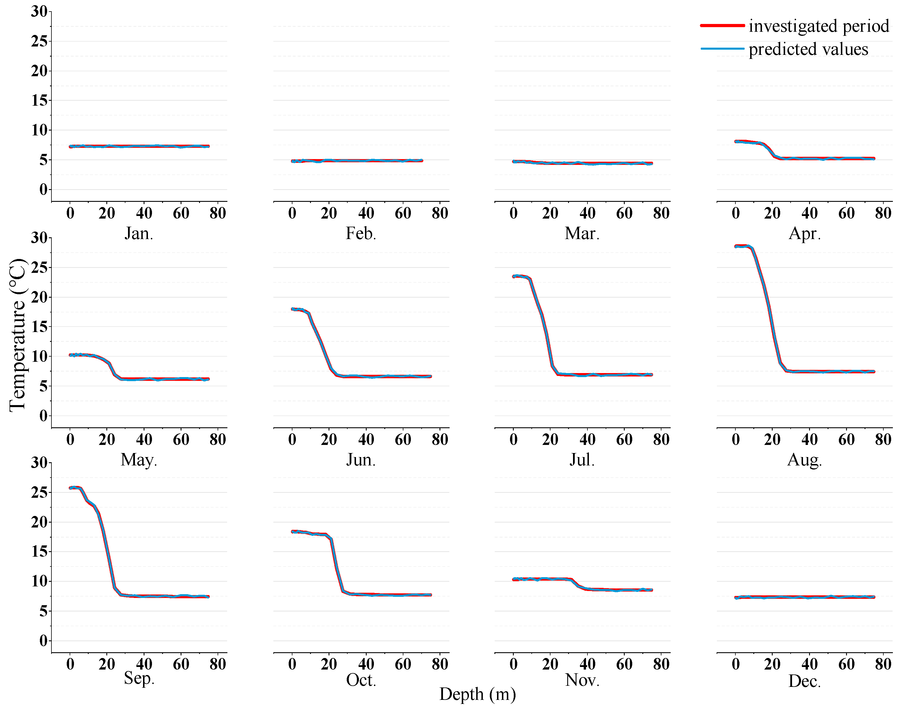
The Ocean-Mixer utilizes historical observations to achieve accurate predictions of ocean temperature in a 3D scenario by capturing the correlation between the time dimension and channels. Figure 8 illustrates the temperature prediction for the next 12 months (from 14 January to 14 December) using data from the previous 36 months, with a prediction step 12. Figure 8 covers data from 0 to 80 m from ocean depths, where the red curve represents the investigated period’s observed temperature values, and the blue curve shows the predicted temperature values.

In Figure 9, the red and blue lines indicate the investigated period and predicted temperature gradients $G$, respectively. Combining Figure 8 and Figure 9, the ocean temperature does not vary much with water depth during January, February, March, and December. However, from April onwards, the temperature fluctuations gradually increase with deeper water depth, especially in July, August, and September, when the temperature fluctuations peak, consistent with the real-world behavior of seasonal variations in the temperate ocean thermocline. This phenomenon also confirms the efficiency of our Ocean-Mixer model in capturing long-term time-series information and temperature trends, as well as its ability to fit nicely into real-world data.

6. Conclusions

In this paper, we propose Ocean-Mixer, a deep learning framework for ocean time series sensing data prediction, which can efficiently capture the correlation between temporal dimensions and channel features by removing redundant temporal information. We first provide an in-depth analysis of the ocean dataset, thus elucidating the importance of eliminating temporal redundant information. Then, the article introduces the three core modules of Ocean-Mixer in detail and describes the entire prediction process in detail. In the experimental section, we apply Ocean-Mixer to the task of thermocline prediction on an ocean dataset and compare it with other models. The results show that Ocean-Mixer performs better on the ocean time series sensing data prediction task and is particularly good at capturing long-term features of the ocean. In addition, we conducted related thermocline experiments, which provide valuable insights and implications for future research.

In future work, we plan to make appropriate improvements to our method and apply it to the classification and prediction of underwater sonar images, as well as to assist in formulating routing strategies for underwater acoustic networks. One possible approach is to integrate convolutional neural networks to handle image information, thereby further capturing the spatial and temporal dependencies in the ocean.