Abstract
Internal solitary waves (ISWs) are large-amplitude internal waves which would destroy underwater engineering. Finding an easy way to discriminate ISWs from field observational data is crucial. Two time--series datasets, one contained ISWs and another only containing internal tides, were obtained from filed observations. Based on single-layer velocity data, wavelet spectrum shows significant high value in short time-scale domain when ISWs pass, whilst having no signal in that domain when only internal tides exist, indicating the capability of wavelet analysis on ISWs detection. Wavelet variances of the dataset with ISWs has a bimodal distribution versus periods with two peaks around 40 min and 110 min, which can also be reproduced by a numerical model, indicating that the energy within period band of 10–120 min is caused by ISWs. By using the conceived signal processing techne, data reconstruction can precisely obtain the arrival time of ISWs and retain about 91.4% of the original signal. It is found that, based on a field observational dataset with even a coarse sampling interval for up to 20 min, the existence of ISWs can be easily discriminated by using wavelet analysis, which provides us an economic method for the early warning of ISWs in ocean engineering.
1. Introduction
Internal solitary waves (ISWs) are large-amplitude, highly nonlinear internal waves active in the stratified ocean. Their amplitudes can reach as large as 240 m in the northern South China Sea, and their induced maximum horizontal speeds can approach 2–3 m/s [1,2,3,4,5]. During their propagation, they can cause a maximum diapycnal mixing rate increase by three orders of magnitude [6]. Also, they can exert large loads on underwater engineering, i.e., oil piles [7,8]. In order to ensure the reliable operation of underwater engineering, it is crucial to alert the arrival of ISWs in advance.
As the largest marginal seas of Pacific, the South China Sea is under the influence of East Asian monsoons, featuring southwest winds in summer and northeast winds in winter [9]. This region is also a typhoon high-incidence area, especially from late spring to early autumn [10], causing severe storm surges in coastal regions of south China [11]. Moreover, mesoscale eddies and the Kuroshio intrusion can also change the stratification in the northeastern South China Sea [12,13], therefore affecting the background shears [14]. Strong tidal waves propagate from the west Pacific into the South China Sea through the Luzon Strait [15]. Both diurnal and semidiurnal tides are dominant in the northeastern South China Sea [16]. The tidal range in this region is affected by bottom topography. It ranges from 1 m near Luzon Strait to over 4 m nearshore.
ISWs are ubiquitous phenomena in the northeast South China Sea [17,18,19,20]. The interaction of strong tidal currents with abrupt underwater topography in the Luzon Strait induces both diurnal and semidiurnal internal tides. Satellite data reveal that semidiurnal internal waves propagate northeastward into the continental shelf, while diurnal internal waves move toward the inner basin [21]. Due to the nonlinear steepening, the internal tides gradually evolve into ISWs [2], which arise from various governing factors such as stratification, currents, fronts, eddies, and topography [22,23,24,25,26,27,28]. The ISWs propagate in the deep basin, disintegrate across the continental slope with a polarity conversion, and ultimately dissipate over the broad continental shelf [29].
ISWs can cause significant isotherms and velocity variations during their passage. Consequently, based on thermistor chain and Acoustic Doppler Current Profiler (ADCP), previous studies used the variations of isotherms or horizontal velocity in the full depth to detect the passage of ISWs. It is much easier to identify ISWs using temperature measurements. Based on the isotherm variations, Gong et al. proposed a temperature superposition method to automatically identify ISWs [30]. When analyzing the field observational data on the Washington continental shelf, Zhang et al. used the variation of the full-depth isotherms to detect the ISWs [26]. Cui et al. took the variation of 17 °C isotherms as an index to figure out the passage of ISW [27]. Chen et al. used the depth displacement of isotherms from 11 to 28 °C to determine the arrival of ISWs [4].
Fewer studies identify ISWs using only velocity data. It is known that during the passage of ISWs, the ISW-induced velocity is opposite in the upper and lower layer ocean. So, the positions of ISWs can be manually found out from a full-depth velocity measurement. Also, the velocity in the upper layer ocean increased largely, but the flow direction remained unchanged when ISWs passed [1]. Shaw et al. suggested that surface convergence with velocity much greater than the maximum barotropic tidal current is a telling sign of the presence of ISWs [31]. Moreover, because the passage time for an ISW is about 20 min, a time-resolution less than 3 min is the recommended measurement interval of instruments. Detection of the passage of ISWs requires a full-depth high-resolution filed observational dataset. In marine engineering, it needs less cost, more efficiency, and higher accuracy to detect ISWs from real-time observations and provide early warnings of the passage of ISWs.
There has been a surge in investigations delving into the dynamics of internal waves, primarily employing power spectra analysis [32,33,34,35,36]. The internal wave field falls within a frequency band f < ω < N, where f is the inertial frequency and N is the buoyancy frequency. Within the frequency band between f and N, a typical spectrum exhibits peaks in the low-frequency range around f, tidal frequencies, and their higher harmonics. These frequency bands facilitate the transfer of energy to higher frequency waves beyond the cutoff frequency at N. The power spectra analysis, relying on Fourier transformation, faces challenges in accurately discerning the frequency of high-frequency signals due to spectral energy leakage. Additionally, the results of Fourier transformations are unable to depict the temporal variation of the data, making it impossible to ascertain the exact time of the passage of ISWs. So, it is difficult to discriminate ISWs using Fourier transformation within the internal wave band. In contemporary research, wavelet analysis is widely used to analyze the variation of power within a time series because it is capable of decomposing the signal both in time and frequency domains, which is better than a Fourier transformation [37]. The wavelet transformation has been used for time-series analysis of numerical model results in geophysics, including El Niño Southern Oscillation [38], wave growth and breaking [39], and internal gravity waves [40]. Considering its capability to get accurate frequency resolution in low-frequency components (long time-scale components) and precise time resolution in high-frequency components (short time-scale components), wavelet analysis is a powerful tool to analyze non-stationary signals.
In this article, based on the field observational data and numerical model results, we propose a method depending on wavelet analysis to discriminate the passage of ISWs using single-layer time-series velocity data near thermocline. This article is organized as follows: the data and methods are presented in Section 2, results are described in Section 3, the discussion is in Section 4, and finally the conclusions are presented in Section 5.
2. Data and Methods
2.1. Field Observation
The field observational data were collected from a mooring located at (117°44.7′ E, 20°44.2′ N) southeast of Dongsha Island from 1 August to 28 September 2014 (Figure 1a). The current velocities were collected by 3 ADCPs with a time sampling resolution of 2 min and a vertical resolution of 16 m from 900 m to sea surface and 8 m from 1180 m to 900 m, respectively. During the observation, ISWs features a fortnightly modulation, i.e., in nearly seven days, two ISWs passed every day and in subsequent seven days, no ISW passed [41]. Thus, we can easily divide the data into two datasets, one contains ISWs, and the other contains only linear internal tides.
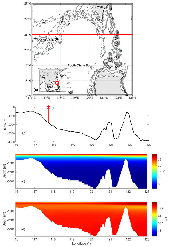
Figure 1.
(a) Bottom topography (depth in meters) in the northern South China Sea, where the red pentagram is the mooring site. The embedded subplot illustrates the geographical location of the study area within Asia, and the red rectangle represents the study domain. Note that the bottom topography within the red rectangle is averaged, as shown in (b) and used in the model. (c) Temperature and (d) salinity obtained from WOA13 are used in the model. The figures here and after are generated by Python version 3.11.8 (https://www.python.org/downloads/windows/, accessed on 6 February 2024).
2.2. Continuous Wavelet Transformation
Continuous wavelet transformation is a powerful tool to reflect the features presented in the time series. It provides temporal-frequency resolution for non-stationary signals, so that it has been widely used in the field of hydrology time-series data analysis [42].
When employing continuous wavelet transformation, the selection of a mother wavelet characterized by unique mathematical properties, such as Gaussian or Morlet, significantly influences the obtained results. In this work, the continuous wavelet transformation is applied utilizing the analytic Morse wavelet as the mother wavelet, which first introduced by Daubechies and Paul [43]. The analytic Morse wavelet has no support on negative frequencies, which makes it capable to capture phase variability accurately [44]. Two parameters, and , associated with the analytic Morse wavelet, control the performance of wavelet analysis. controls the low-frequency behaviors, and controls the high-frequency decay, respectively [45]. Increasing with fixed appears to pack more oscillations into the same envelope, whereas increasing with fixed additionally modifies the function shape, with the function modulus curves becoming less strongly concentrated on its center. According to the shape of ISW-induced velocity with time, we set equals to 3 and equals to 10, respectively.
To get the distribution of wave energy versus period, the wavelet variance was also calculated. Wavelet variance decomposes the variance of a time series into components associated with different scales. It can be used to identify the dominant period of the signal and their relative strength at different periods.
2.3. Setup of the Numerical Model
A two-dimensional fully nonlinear, non-hydrostatic Massachusetts Institute of Technology general circulation model (MITgcm) was applied to model the generation and evolution process of ISWs in the northern South China Sea. The MITgcm solves the incompressible Boussinesq non-hydrostatic Navier–Stokes equations, and the dynamic equations used in the model are described as follows:
where is the vector of velocity, b is the buoyancy, is non-hydrostatic parameter, and , , and are surface, hydrostatic, and non-hydrostatic pressure terms, respectively. The represent advective, metric, and Coriolis terms in the momentum equations. In spherical coordinates, they have the form:
where is the earth rotation, is the latitude, and is the forcing and dissipation terms in horizontal and vertical direction. For full detail, please refer to Marshell et al. [46].
In this work, the model domain was from 116° E to 123° E, where ISWs emerge from nonlinear steepening of internal tidal waves and then gradually split into a rank-ordered ISW packet. The bottom topography used here was averaged from 20° N to 21° N (rectangle showed in Figure 1a) extracted from GEBCO2020 (https://www.gebco.net/data_and_products/gridded_bathymetry_data/ gebco_2020, accessed on 6 February 2024) with a spatial resolution of 15″. The maximum water depth in the model was 3950 m (Figure 1b). The horizontal resolution was set to 150 m, and the vertical resolution was 10 m in the upper 300 m and gradually varied to 100 m. The total number of grid points was 5376 × 88, and the time step as set to 10 s. The initial horizontal temperature and salinity data in August were derived from the climatological month-mean data of World Ocean Atlas (2013) (Figure 1c,d). To avoid the reflections of wave in both open boundaries, sponge layers were implemented in 30 grid points near each open boundary. The model was driven at the eastern boundary by M2 barotropical tide with an amplitude of 0.05 m/s. The background viscosity and diffusivity were set at a constant value of 10−5 m2s−1.
3. Results
To obtain which period band the ISWs’ energy is concentrated, two velocity datasets taken from field observation data at 60 m are used for analysis: one is from 10 August to 17 August containing 24 ISW events (Figure 2a), and the other from 18 August to 25 August containing only linear internal tides (Figure 2c). By comparing these two datasets, internal tidal signals with an amplitude of 0.5 m/s are pronounced in both datasets. But when ISWs pass, the velocity suddenly increases with a maximum velocity reaching 2.52 m/s. And the passage time of a single ISW ranged from 20 min to 47 min in this dataset, depending on the variable amplitude of each ISW. A single ISW and rank-ordered ISW packets with two or three solitons alternate with each other at an interval of near 12 h a day. Figure 2b,c are the continuous wavelet power spectra of the above two datasets. High values in continuous wavelet power spectra indicate where the energy is concentrated. In both cases, the maximum energy lies in long time-scale domain with a peak around 1410 min, revealing that diurnal currents are dominant at the observational site, which are suggested by previous studies [47]. However, in the short time-scale domain, significant differences can be seen. When ISWs pass, notable peaks are observed in the short time-scale domain of the wavelet spectrum. These spike-like peaks indicate a concentration of pronounced energy during the passage of ISWs in the short time-scale domain. Conversely, the wavelet spectrum reveals a tendency for energy to concentrate in the long time-scale domain when only internal tides are presented. A high value in the short time-scale domain of wavelet spectrum is a telling sign of ISWs. Wavelet transformation can easily discriminate nonlinear ISWs from linear internal waves.
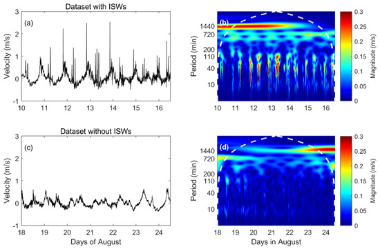
Figure 2.
(a) Time series of current velocity with ISWs from 10 August to 17 August at 60 m. The positive value means westward velocity and the negative means eastward one, respectively. (b) Continuous wavelet power spectra of (a); (c) is the same as (a), but without ISWs from 18 August to 25 August at 60 m; (d) continuous wavelet power spectra of (c). The white dashed-lines in (b,d) indicate the region that was affected by the edge of the data.
Figure 3 shows the wavelet variances versus the period of current velocity datasets with ISWs and without ISWs. It can be easily found that the wavelet variances of both datasets have peak values around periods of 24 h, 12 h, and 8 h, which reveals the diurnal tide, semi-diurnal tide, and its harmonic components. The main difference between the wavelet variances with ISWs and without ISWs lies in the short time-scale part of the curve. When there exist ISWs, a bimodal distribution versus period can be found in a time-scale shorter than 200 min (Figure 3b). The wavelet variances peak around periods of 40 min and 110 min in short time-scale, respectively. In contrast, wavelet variance is mild when no ISWs pass. It can be inferred that the energy of ISWs concentrates around periods of approximately 40 min and 110 min at our observation site. It is noteworthy that two curves are almost coincident at periods shorter than 10 min, indicating that the energy at periods shorter than 10 min may not be attributed by ISWs.
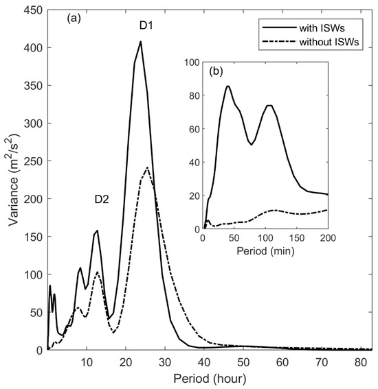
Figure 3.
(a) Wavelet variances of current velocity dataset with ISWs (solid line) and without ISWs (dashed line) versus period. The subplot (b) is the enlargement of (a) in a period of 0–200 min.
Since the observational data contain multiple time-scale processes, to get a pure signal of ISWs, a nonlinear numerical model forced solely by M2 tidal component is applied to model the propagation of ISWs. Figure 4a shows the modeled velocity at 1 min time resolution obtained at the same site of the mooring. In the numerical model, only the signals of internal tides and ISWs are significant. It can be clearly seen that the ISWs appear at an interval of 12.42 h, traveling as a single soliton with a maximum westward wave-induced velocity exceeding 1.5 m/s. The same as that in the observation, wavelet transformation is applied to the modeled velocity data at 60 m (Figure 4b). The maximum value of continuous wavelet power spectra lies in long time-scale domain around 720 min, indicating the existence of semi-diurnal internal tides. When ISWs pass, significant high values emerge in a short time-scale domain. Figure 4c presents the wavelet variance of the model results. A bimodal distribution versus period is significant in short time-scale with peak values lying around 40 min and 110 min, respectively, which is consistent with that of filed observation. Moreover, the value of wavelet variance equals zero at periods shorter than 10 min, revealing that no energy concentrated in this time scale in the numerical model. It confirms that signals with periods shorter than 10 min in the observation are not caused by ISWs.
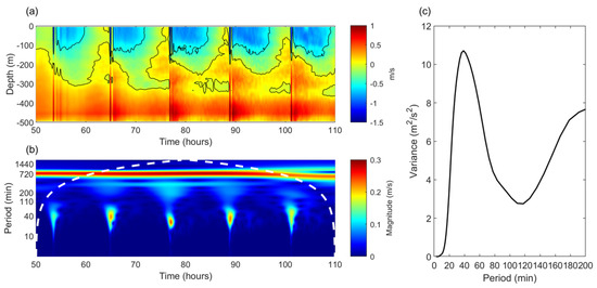
Figure 4.
(a) Time series of modeled horizontal current velocity at a time resolution of 1 min with depth at 117.5° E. (b) is the continuous wavelet power spectra of modeled velocity at a depth of 60 m, and (c) is the corresponding wavelet variances of modeled current velocity versus period. The white dashed-line in (b) indicates the region that is affected by the edge of the data.
As mentioned above, the ISWs exhibit distinctive properties in the wavelet-transformed field, rendering them detectable through wavelet transformation. To get the arrival time of ISWs and the maximum ISW-induced velocity precisely, a conceived signal processing technique is proposed. It is comprised of five stages, as follows:
- (1)
- Selection of Velocity Time−Series Data
The time-series velocity data near the depth of thermocline are chosen. This selection is motivated by the fact that the ISW-induced velocity reaches its maximum in the upper ocean, rendering the signal more significant compared to that in the deep ocean. It is noteworthy that the selection of the dataset will significantly influence the detection results. A continuous wavelet transformation with an analytic Morse mother wavelet is applied to the chosen single-layer data.
- (2)
- Reduction of Wavelet Components
According to the above analyses indicating that predominant periods, approximately 40 min and 110 min, are primarily caused by ISWs, a reduction of wavelet components is performed. The magnitude of continuous wavelet power spectra beyond the time band from 10 to 120 min (i.e., the frequency band from 1.39 × 10⁻⁴ to 1.7 × 10⁻³ Hz) is set to 0. It is worth noting that this time band is specified for ISW events. It will not change when applying to the dataset obtained from other sea areas. This will be discussed in detail in Section 4.
- (3)
- Hard Threshold Application
A hard threshold based on 3−sigma rule is adopted before signal reconstruction. The magnitude of continuous wavelet power spectra with absolute values lower than the threshold are set to zero. The threshold value in our study is equal to 68.62%.
- (4)
- Signal Reconstruction
Signal reconstruction is through inverse wavelet transform. By using the same mother wavelet setup, a new velocity time-series is formed.
- (5)
- Peak Value Localization
Peak values and their corresponding times in the reconstruction data are located, which represent the maximum ISW-induced velocity and the arriving time of ISWs, respectively.
Figure 5 illustrates the comparison of the original velocity time-series and the output of the signal reconstruction with and without ISWs, respectively. The original data are composed of different time scales, including internal tides, ISWs, and high-frequency waves. When ISWs pass, the velocity increases significantly. However, not all the velocity increases are caused by ISWs, e.g., on 11 August, the maximum velocity reaches 0.9 m/s, but there is no ISW structure according to the variations of isotherms. By applying signal processing, the ISW signal can be easily detected from various signals. Especially, the passage of each soliton in an ISW packet can be discriminated.
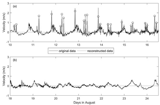
Figure 5.
Comparison of original dataset (solid lines) with reconstructed dataset (dashed lines) (a) with ISWs and (b) without ISWs. The circles in (a) show the extrema of the reconstruction data.
For a detailed comparison between our method and traditional approaches, we used/the traditional ISW detective method using the full-depth velocity data. The identification of ISWs is based on the vertical structure of waves, and the maximum ISW-induced velocity is determined by subtracting the background velocity from the maximum velocity observed during the passage of the ISWs. Subsequently, the maximum ISW-induced velocity mentioned in the following paragraph is obtained through the traditional method, while the reconstruction velocity denotes the velocity obtained using our method.
The arrival time of maximum ISW-induced velocity is precisely obtained, and the reconstructed velocity can retain over 90% of the original signal. For example, on 13 August, a maximum ISW-induced velocity was recorded. The background velocity before the wave arrived was 0.19 m/s, and the maximum velocity when the ISW passed was 2.48 m/s, indicating that the ISW-induced velocity is about 2.29 m/s. The reconstructed velocity was 2.18 m/s, which retains 95.1% of the original velocity. Table 1 shows the comparison of the original ISW-induced velocity and the reconstructed velocity. It can be found that the reconstructed velocity can retain at least 70% of the original ISW-induced velocity. The average ratio reaches 91.4%. Furthermore, the signal processing is applied to the time series without ISWs. The reconstructed velocity consistently remains zero, illustrating that our signal processing technique is effective to filter linear internal tides and high-frequency waves in the filed observation. Although traditional methods may offer a more accurate means of obtaining the maximum ISW-induced velocity, our new method excels in its ability to automatically detect ISWs and determine the maximum ISW-induced velocity. This automated approach enhances efficiency and reduces costs associated with manual interventions.

Table 1.
Comparison Of ISW-Induced Velocity And The Reconstructed Velocity (Unit: m/s).
It is noticed that, in the field observation, a high sampling interval results in a high cost of observation. It is interesting to ask whether a coarse sampling interval can catch the signal of ISW events by using wavelet analysis. Here, we take the ISW-induced velocity time series at the depth of 60 m from 8 August to 13 August as an example. Various sampling intervals of 6, 10, 20, and 30 min are chosen to compute the wavelet variances (Figure 6a). For comparison, the wavelet variances without ISWs are also calculated at different sampling intervals (Figure 6c). It can be found that the wavelet variances at different sampling intervals with or without ISWs exhibit peak values around periods of 24 h, 12 h, and 8 h, though the peak values become smaller as the sampling interval increases. This is because the energy leaks when the sampling intervals are coarse. At periods less than 200 min, a clear bimodal distribution versus period, with peaks near 40 min and 110 min, can be seen when sampling intervals are 6 min and 10 min, respectively (Figure 6b). As the sampling intervals increase, the bimodal structure of wavelet variance gradually vanishes. Particularly, when the sampling interval increase to 20 min, which is about the half of the passage time of ISWs, a significantly high value can also be found near a period of 40 min, indicating that the existence of the ISWs can be easily discriminated from field observational data with a 20 min sampling interval. However, when the sampling interval increases to 30 min, no notable signal can be seen at periods between 10 and 120 min. In contrast, when there is no ISWs, the wavelet variances always keep mild at periods less than 200 min, no matter what the sampling interval is. All in all, when the sampling interval is less than 20 min, which is about half the passage time of a single ISW, the field observational data can be used to discriminate the ISW events by using wavelet analysis.
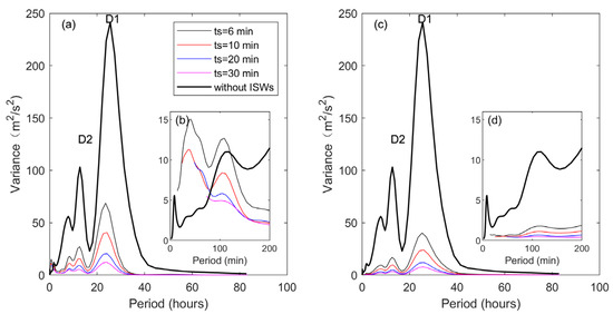
Figure 6.
(a) Wavelet variances of current velocity dataset with ISWs at re-sampled time resolutions of 5 min (black), 10 min (red), 20 min (blue), and 30 min (magenta), respectively. The subplot (b) is the enlargement of (a) during 0–200 min; (c) and (d) are the same as (a) and (b), but using the current velocity dataset without ISWs. The heavy black line represents the wavelet variance of current velocity dataset without ISWs at an original time resolution of 2 min.
4. Discussion
To assess the adaptability of our method, an additional velocity dataset with a time resolution of 15 min was employed to identify the passage of ISWs. The velocity data were acquired from a bottom-mounted Acoustic Doppler Current Profiler (ADCP) on the Oregon continental shelf (−124.3054° E, 44.64068° N) during a period from 15 July to 28 July 2015 (data available at https://oceanobservatories.org/, accessed on 6 February 2024). The Oregon continental shelf is recognized as a hotspot for ISWs [48,49]. Figure 7a depicts the eastward velocity at the mooring, revealing the passage of eight ISW packets at the observation site, where the upper layer velocity flows eastward while the lower velocity moves in an opposite direction.
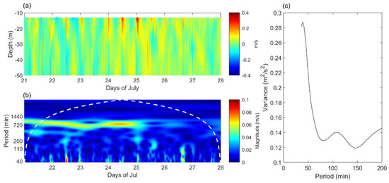
Figure 7.
(a) Time series of horizontal current velocity at a time resolution of 15 min obtained on the Oregon continental shelf. (b) is the continuous wavelet power spectra of the velocity at a depth of 25 m, and (c) is the corresponding wavelet variances of the current velocity versus period. The white dashed-line in (b) indicates the region that is affected by the edge of the data.
After applying continuous wavelet transformation to the velocity at 20 m, pronounced high values emerge in the short time-scale domain (Figure 7b). The wavelet variance of the velocity dataset exhibits a bimodal distribution versus periods with two peaks around 40 min and 110 min, respectively, consistent with those from the South China Sea dataset. This confirms that the energy within a period band of 10–120 min is induced by ISWs, validating the universality of the parameters employed in our method for ISWs detection irrespective of the observation location.
Despite the original data having a time resolution of 15 min, our method successfully detected seven out of eight ISWs, yielding a 12.5% missed detection rate. The reconstructed velocity retained an average of 85.4% of the original ISW-induced velocity (see Table 2). This example with a coarse time resolution illustrates that our method is economic in detecting ISWs, since the ISWs can be easily obtained from single-layer velocity observation with a coarse time resolution.
Table 2.
Comparison of the ISW-Induced Velocity with the Reconstructed Velocity (Unit: m/s).
5. Conclusions
In this paper, wavelet analysis is employed to analyze the ISW signals obtained from field observational data and modeled results. Despite the time and frequency resolution, problems exist regardless of the transforms used, as it is difficult to discriminate ISW signals from internal wave communities using Fourier Transformation. Because wavelet analysis is capable of presenting high time resolution at high frequency, it becomes a powerful tool to analyze the non-stationary signals like ISWs. Based on high time resolution field observational data, two time-series datasets, one containing ISWs and the other featuring only linear internal tidal signals, are obtained. By applying wavelet transformation, high values appear in the short time-scale domain of continuous wavelet power spectra when ISWs pass, whilst no signal appears in that domain when there are only internal tides. The wavelet variances show that the energy of ISWs predominantly concentrates at periods near 40 min and 110 min. A bimodal structure is clearly seen in wavelet variances below 200 min. This bimodal structure can also be reproduced by the numerical model. It is noted that the energy at periods shorter than 10 min is not caused by ISWs. Only energy within a period band of 10–120 min is attributed by ISWs. Once the period band of ISWs is determined, the maximum ISW-induced velocity and the exact arrival time of ISWs can be identified by using a conceived signal processing technique. The reconstructed velocity can retain an average fidelity of 91.4% when compared with the original one. Moreover, different sampling intervals of 6, 10, 20, and 30 min are also used to compute the wavelet variances. Results show that a field observational dataset with even a coarse sampling interval for up to 20 min can also be used to discriminate the signal of ISWs, which may provide us a lower cost observation strategy for the early warning of ISWs in ocean engineering.
Author Contributions
Conceptualization, J.X. and S.C. (Shuqun Cai); Formal analysis, S.C. (Shaomin Chen), Y.G. and D.L.; Writing—Original Draft, J.X.; Writing—Review and Editing, Z.C. and S.C. (Shuqun Cai); Visualization, J.X.; Foundation acquisition, J.X. and S.C. (Shuqun Cai). All authors have read and agreed to the published version of the manuscript.
Funding
This research was funded by the National Natural Foundation of China (NSFC) under grant numbers 42130404, 42276022, and 42206012. Science and Technology Projects in Guangzhou under grant number 2024A04J9022.
Data Availability Statement
The data presented in this study are available on request from the corresponding author. And data in discussion section is publicly available datasets which can be found here: https://oceanobservatories.org/ (accessed on 1 February 2024).
Conflicts of Interest
All authors declare no conflicts of interest.
References
- Cai, S.Q.; Gan, Z.J.; Long, X.M. Some characteristics and evolution of the internal soliton in the northern South China Sea. Chin. Sci. Bull. 2002, 47, 21–27. [Google Scholar] [CrossRef]
- Alford, M.; Peacock, T.; Mackinnon, J.; Nash, J.; Buijsman, M.; Centuroni, L.; Chao, S.; Chang, M.; Farmer, D.; Fringer, O.; et al. The formation and fate of internal waves in the South China Sea. Nature 2015, 521, 65–69. [Google Scholar] [CrossRef]
- Huang, X.; Chen, Z.; Zhao, W.; Zhang, Z.; Zhou, C.; Yang, Q.; Tian, J. An extreme internal solitary wave event observed in the northern South China Sea. Sci. Rep. 2016, 6, 30041. [Google Scholar] [CrossRef]
- Chen, L.; Zheng, Q.; Xiong, X.; Yuan, Y.; Xie, H.; Guo, Y.; Yu, L.; Yun, S. Dynamic and Statistical Features of Internal Solitary Waves on the Continental Slope in the Northern South China Sea Derived From Mooring Observations. J. Geophys. Res. Oceans 2019, 124, 4078–4097. [Google Scholar] [CrossRef]
- Ramp, S.R.; Park, J.H.; Yang, Y.J.; Bahr, F.; Jeon, C. Latitudinal Structure of Solitons in the South China Sea. J. Phys. Oceanogr. 2019, 49, 1747–1767. [Google Scholar] [CrossRef]
- Xu, J.; Xie, J.; Chen, Z.; Cai, S.; Long, X. Enhanced mixing induced by internal solitary waves in the South China Sea. Cont. Shelf Res. 2012, 49, 34–43. [Google Scholar] [CrossRef]
- Cai, S.; Long, X.; Gan, Z. A method to estimate the forces exerted by internal solitons on cylindrical piles. Ocean Eng. 2003, 30, 673–689. [Google Scholar] [CrossRef]
- Xie, J.; Xu, J.; Cai, S. A numerical study of the load on cylindrical piles exerted by internal solitary waves. J. Fluids Struct. 2011, 27, 1252–1261. [Google Scholar] [CrossRef]
- Hu, J.; Kawamura, H.; Hong, H.; Kobashi, F.; Wang, D. 3≈6 Months Variation of Sea Surface Height in the South China Sea and Its Adjacent Ocean. J. Oceanogr. 2001, 57, 69–78. [Google Scholar] [CrossRef]
- Wu, R.; Li, C. Upper ocean response to the passage of two sequential typhoons. Deep Sea Res. Part I 2018, 132, 68–79. [Google Scholar] [CrossRef]
- Pun, I.-F.; Chan, J.; Lin, I.; Chan, K.; Price, J.; Ko, D.; Lien, C.; Wu, Y.; Huang, H. Rapid Intensification of Typhoon Hato (2017) over Shallow Water. Sustainability 2019, 11, 3709. [Google Scholar] [CrossRef]
- Chen, G.; Hou, Y.; Chu, X. Mesoscale eddies in the South China Sea: Mean properties, spatiotemporal variability, and impact on thermohaline structure. J. Geophys. Res. 2011, 116, C06018. [Google Scholar] [CrossRef]
- Nan, F.; Xue, H.; Yu, F. Kuroshio intrusion into the South China Sea: A review. Prog. Oceanogr. 2015, 137, 314–333. [Google Scholar] [CrossRef]
- Zhang, Z.; Tian, J.; Qiu, B.; Zhao, P.; Chang, D.; Wu, D.; Wan, X. Observation 3D structure, generation and dissipation of oceanic mesoscale eddies in the South China Sea. Sci. Rep. 2016, 6, 24349. [Google Scholar] [CrossRef]
- Zhao, J.; Zhang, Y.; Liu, Z.; Zhao, Y.; Wang, M. Seasonal variability of tides in the deep northern South China Sea. Sci. China Earth Sci. 2019, 62, 671–683. [Google Scholar] [CrossRef]
- Zu, T.; Gan, J.; Erofeeva, S.Y. Numerical study of the tide and tidal dynamics in the South China Sea. Deep Sea Res. Part I 2008, 55, 137–154. [Google Scholar] [CrossRef]
- Lai, Z.G.; Jin, G.Z.; Huang, Y.M.; Chen, H.Y.; Shang, X.D.; Xiong, X.J. The Generation of Nonlinear Internal Waves in the South China Sea: A Three−Dimensional, Nonhydrostatic Numerical Study. J. Geophys. Res. 2019, 124, 8949–8968. [Google Scholar] [CrossRef]
- Lamb, K.G.; Lien, R.-C.; Diamessis, P.J. Internal Solitary Waves and Mixing. In Encyclopedia of Ocean Sciences; Academic Press: Cambridge, MA, USA, 2019; pp. 533–541. [Google Scholar]
- Huang, X.D.; Zhang, Z.W.; Zhang, X.J.; Qian, H.B.; Zhao, W.; Tian, J.W. Impacts of a Mesoscale Eddy Pair on Internal Solitary Waves in the Northern South China Sea revealed by Mooring Array Observations. J. Phys. Oceanogr. 2017, 47, 1539–1554. [Google Scholar] [CrossRef]
- Jackson, C. Internal wave detection using the moderate resolution Imaging spectroradiometer (MODIS). J. Geophys. Res. 2007, 112, C11012. [Google Scholar] [CrossRef]
- Zhao, Z. Internal tide radiation from the Luzon Strait. J. Geophys. Res. Oceans 2014, 119, 5434–5448. [Google Scholar] [CrossRef]
- Giese, G.S.; Hollander, R.B.; Fancher, J.E.; Giese, B.S. Evidence of coastal seiche excitation by tide-generated internal solitary waves. Geophys. Res. Lett. 1982, 9, 1305–1308. [Google Scholar] [CrossRef]
- Giese, G.S.; Hollander, R.B. The relationship between coastal seiches at Palawan Island and tide-generated internal waves in the Sulu Sea. J. Geophys. Res. 1987, 92, 5151–5156. [Google Scholar]
- Giese, G.S.; Chapman, D.C.; Black, P.G.; Fornshell, J.A. Causation of large-amplitude coastal seiches on the Caribbean coast of Puerto Rico. J. Phys. Oceanogr. 1990, 20, 1449–1458. [Google Scholar] [CrossRef][Green Version]
- Zhang, X.; Huang, X.; Zhang, Z.; Zhou, C.; Tian, J.; Zhao, W. Polarity Variations of Internal Solitary Waves over the Continental Shelf of the Northern South China Sea: Impacts of Seasonal Stratification, Mesoscale Eddies, and Internal Tides. J. Phys. Oceanogr. 2018, 48, 1349–1365. [Google Scholar] [CrossRef]
- Zhang, S.; Alford, M.; Mickett, J. Characteristics, generation and mass transport of nonlinear internal waves on the Washington continental shelf. J. Geophys. Res. Oceans 2015, 120, 741–758. [Google Scholar] [CrossRef]
- Cui, Z.; Liang, C.; Lin, F.; Jin, W.; Ding, T.; Wang, J. The observation and analysis of the internal solitary waves by mooring system in the Andaman Sea. J. Mar. Sci. 2020, 38, 16–25. [Google Scholar]
- Huang, S.; Huang, X.; Zhao, W.; Chang, Z.; Xu, X.; Yang, Q.; Tian, J. Shear Instability in Internal Solitary Waves in the Northern South China Sea Induced by Multiscale Background Processes. J. Phys. Oceanogr. 2022, 52, 2975–2994. [Google Scholar] [CrossRef]
- Bai, Y.; Song, H.; Guan, Y.; Yang, S. Estimating depth of polarity conversion of shoaling internal solitary waves in the northeastern South China Sea. Cont. Shelf Res. 2017, 143, 9–17. [Google Scholar] [CrossRef]
- Gong, Q.; Chen, L.; Diao, Y.; Xiong, X.; Sun, J.; Lv, X. On the identification of internal solitary waves from moored observations in the northern South China Sea. Sci. Rep. 2023, 13, 3133. [Google Scholar] [CrossRef]
- Shaw, P.; Ko, D.; Chao, S. Internal solitary waves induced by flow over a ridge: With applications to the northern South China Sea. J. Geophys. Res. 2009, 114, C02019. [Google Scholar]
- Xing, J.; Davies, A. Nonlinear effects of internal tides on the generation of tidal mean flow at the Hebrides shelf edge. Geophys. Res. Lett. 2001, 28, 3939–3942. [Google Scholar] [CrossRef]
- Van Haren, H. On the nature of internal wave spectra near a continental slope. Geophys. Res. Lett. 2002, 29, 121615. [Google Scholar] [CrossRef]
- Van Haren, H. Current spectra under varying stratification conditions in the central North Sea. J. Sea Res. 2004, 51, 77–91. [Google Scholar] [CrossRef]
- Van Haren, H. Tidal and near-inertial peak variations around the diurnal critical latitude. Geophys. Res. Lett. 2005, 32, L23611. [Google Scholar] [CrossRef]
- Carter, G.; Gregg, M. Persistent near-diurnal internal waves observed above a site of M2 barotropic-to-baroclinic conversion. J. Phys. Oceanogr. 2006, 36, 1136–1147. [Google Scholar] [CrossRef]
- Torrence, C.; Gilbert, P. A Practical Guide to Wavelet Analysis. Bull. Am. Meteorol. Soc. 1998, 79, 61–78. [Google Scholar] [CrossRef]
- Detto, M.; Joseph, W.; Calderón, O.; Helene, C. Resource acquisition and reproductive strategies of tropical forest in response to the El Niño–Southern Oscillation. Nat. Commun. 2018, 9, 913. [Google Scholar] [CrossRef]
- Liu, P.C. Wavelet spectrum analysis and ocean wind waves. Wavel. Geophys. 1994, 4, 151–166. [Google Scholar]
- Hawkins, J.; Warn−Varnas, A.; Christov, I. Fourier, scattering, and wavelet transforms: Application to internal gravity waves with comparisons to linear tidal data. In Nonlinear Time Series Analysis in the Geosciences; Donner, R., Barbosa, S., Eds.; Springer: Berlin/Heidelberg, Germany, 2008; Volume 112, pp. 223–244. [Google Scholar]
- Xu, J.; He, Y.; Chen, Z.; Zhan, H.; Wu, Y.; Xie, J.; Shang, X.; Ning, D.; Fang, W.; Cai, S. Observations of different effects of an anti-cyclonic eddy on internal solitary waves in the South China Sea. Prog. Oceanogr. 2020, 188, 102422. [Google Scholar] [CrossRef]
- Moradi, M. Wavelet transform approach for denoising and decomposition of satellite-derived ocean color time-series: Selection of optimal mother wavelet. Adv. Space Res. 2022, 69, 2724–2744. [Google Scholar] [CrossRef]
- Daubechies, I.; Paul, T. Time-frequency localisation operators: A geometric phase space approach II. The use of dilations and translations. Inverse Probl. 1988, 4, 661–680. [Google Scholar] [CrossRef]
- Lilly, J.M.; Olhede, S.C. Higher-order properties of analytic wavelets. IEEE Trans. Signal Process. 2009, 57, 146–160. [Google Scholar] [CrossRef]
- Lilly, J.M.; Olhede, S.C. Generalized Morse wavelets as a superfamily of analytic wavelets. IEEE Trans. Signal Process. 2012, 60, 6036–6041. [Google Scholar] [CrossRef]
- Marshall, J.; Hill, C.; Perelman, J.; Adcroft, A. Hydrostatic, quasi-hydrostatic, and nonhydrostatic ocean modeling. J. Geophys. Res. 1997, 102, 5733–5752. [Google Scholar] [CrossRef]
- Xie, X.; Liu, Q.; Zhao, Z.; Shang, X.; Cai, S.; Wang, D.; Chen, D. Deep sea currents driven by breaking internal tides on the continental slope. Geophys. Res. Lett. 2018, 45, 6160–6166. [Google Scholar] [CrossRef]
- Stanley, J.; Holman, R.A.; Barth, J.A.; Suanda, S.H. Shore−Based Video Observations of Nonlinear Internal Waves across the Inner Shelf. J. Atmos. Ocean. Tech. 2014, 31, 714–728. [Google Scholar]
- Lien, R.-C.; D’Asaro, E.A.; Henyey, F. High–Frequency Internal Waves on the Oregon Continental Shelf. J. Phys. Oceanogr. 2007, 37, 1956–1967. [Google Scholar]


Disclaimer/Publisher’s Note: The statements, opinions and data contained in all publications are solely those of the individual author(s) and contributor(s) and not of MDPI and/or the editor(s). MDPI and/or the editor(s) disclaim responsibility for any injury to people or property resulting from any ideas, methods, instructions or products referred to in the content. |
© 2024 by the authors. Licensee MDPI, Basel, Switzerland. This article is an open access article distributed under the terms and conditions of the Creative Commons Attribution (CC BY) license (https://creativecommons.org/licenses/by/4.0/).