
Distribution of Suitable Habitats for Soft Corals (Alcyonacea) Based on Machine Learning

 ,
,
Abstract
1. Introduction
2. Materials and Methods
2.1. Materials
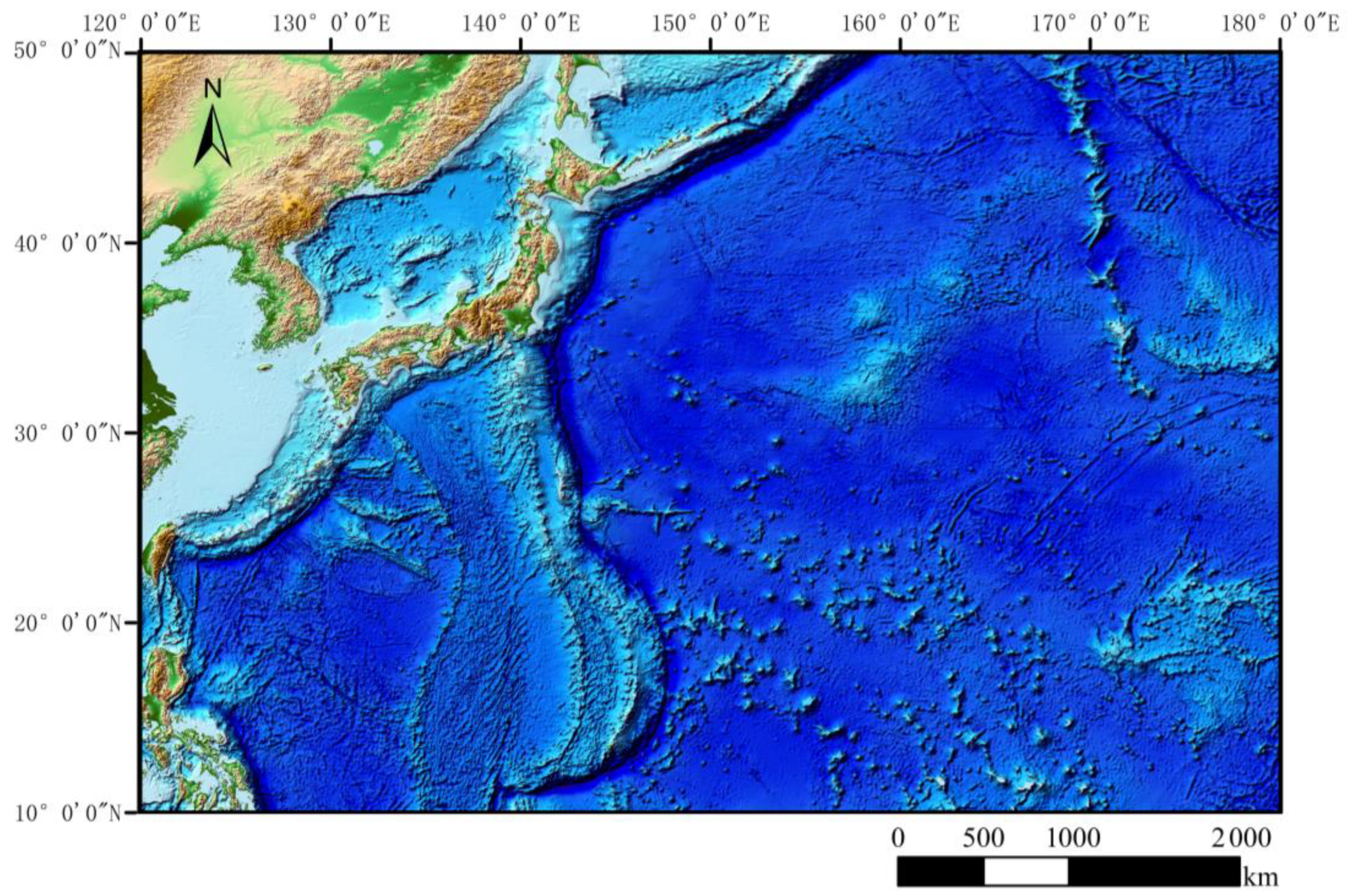
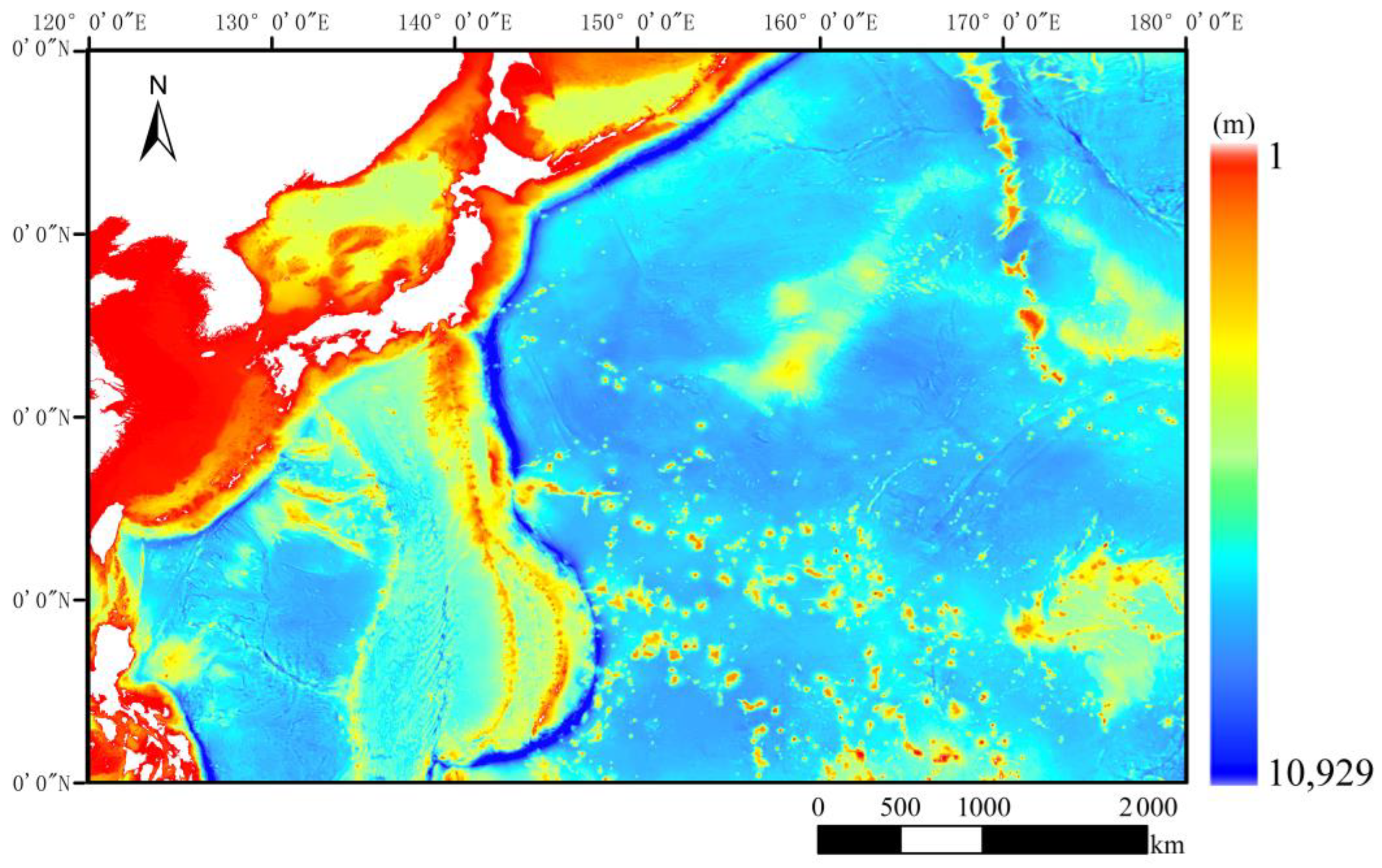
2.1.1. Study Area
2.1.2. Different Species Distribution Models
- 1.
- Maximum entropy models
- 2.
- Random forest models
- 3.
- Artificial neural network models
- 4.
- The XGBoost model
2.2. Data Sources
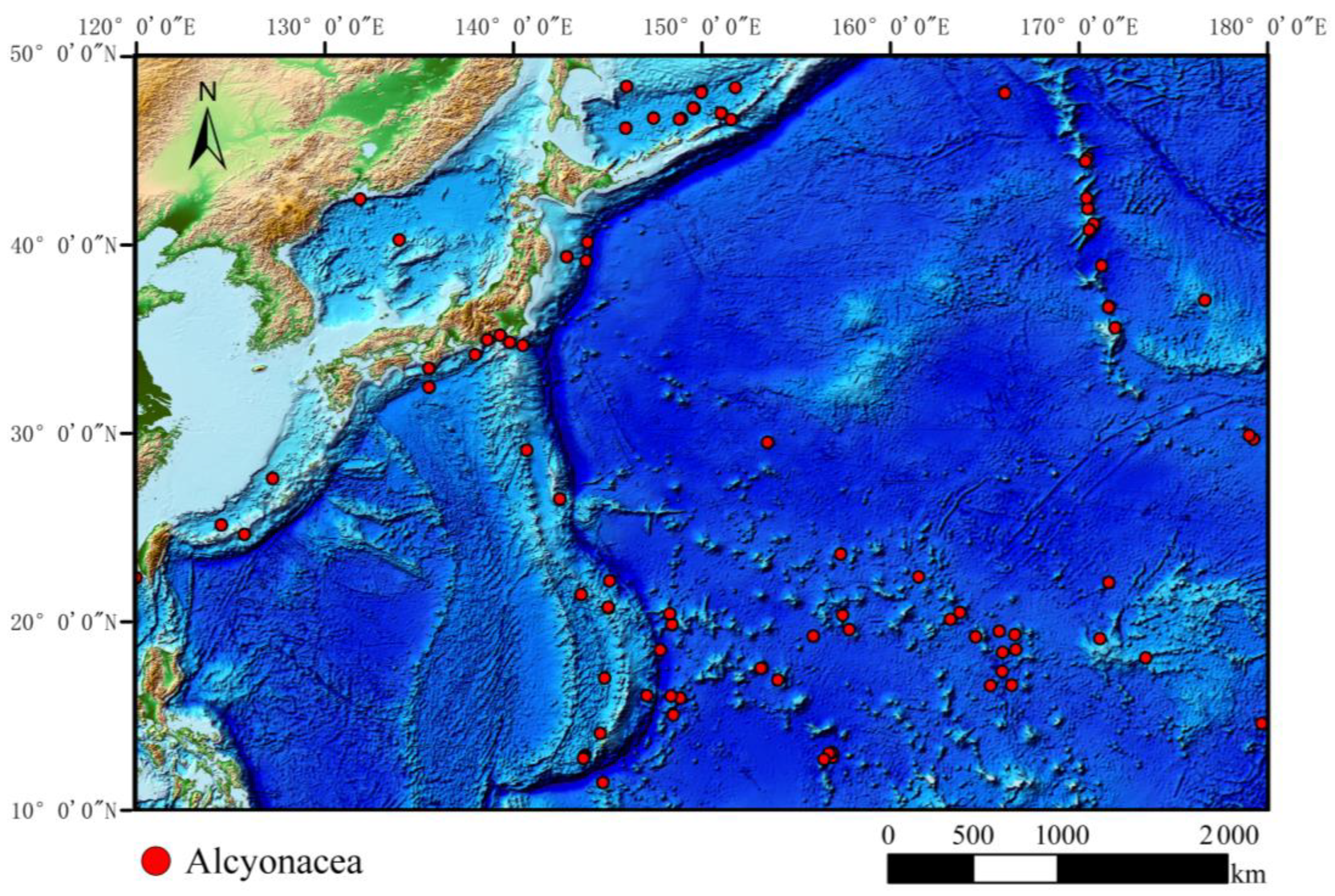
2.2.1. Species Distribution Data
2.2.2. Data on Marine Environmental Variables
2.3. Construction of 15 Arc Sec Resolution Marine Environmental Dataset and Sample Data Establishment
2.3.1. Marine Environmental Dataset
2.3.2. Species Distribution Data Processing
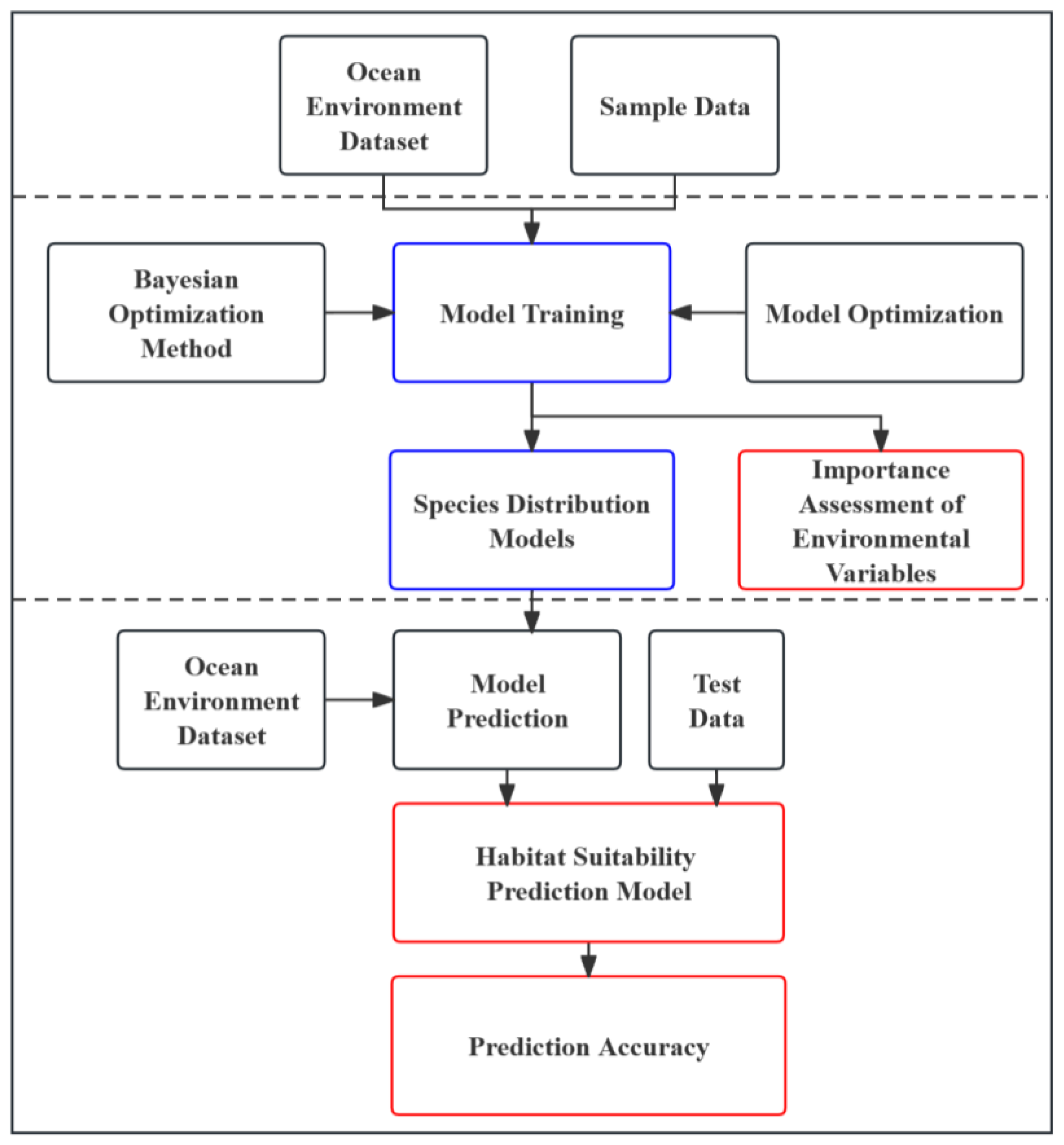
2.4. Model Framework
2.4.1. Construction of Training Dataset
2.4.2. Model Training
2.4.3. Model Prediction
2.5. Model Assessment
3. Results
3.1. Statistical Comparison of Model Performance
3.2. Predicted Distribution of Species
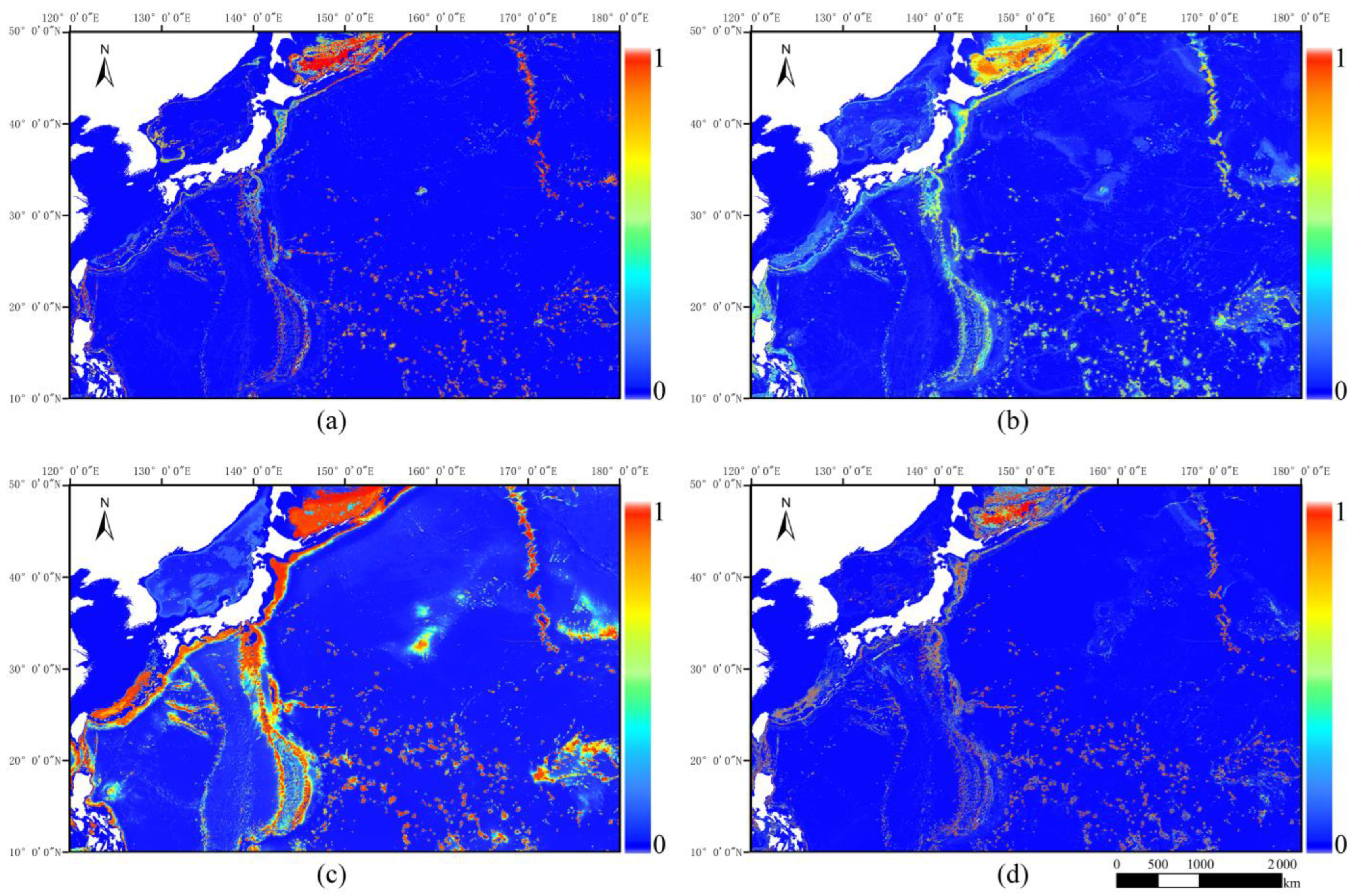
3.2.1. Potential Distribution Projections
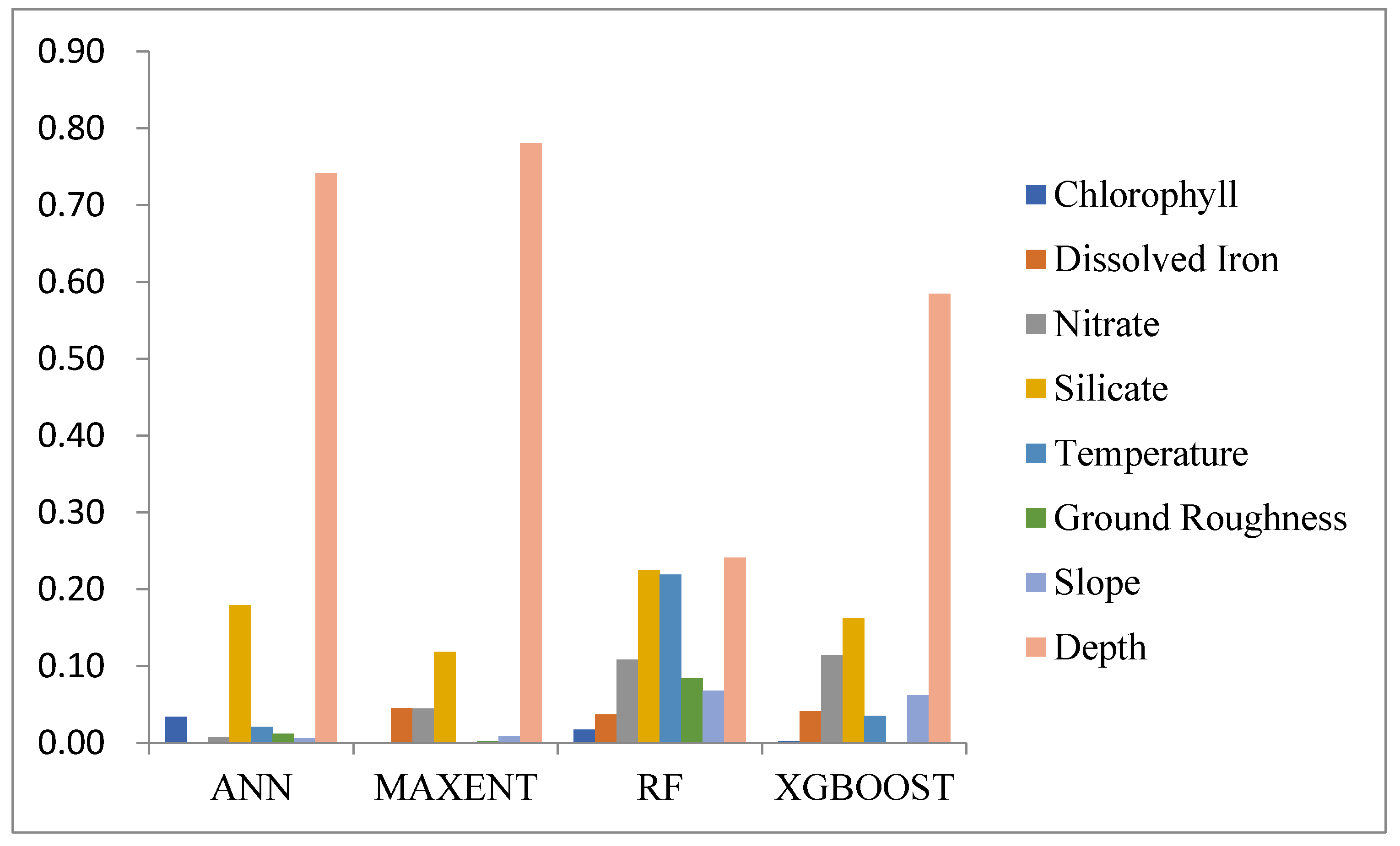
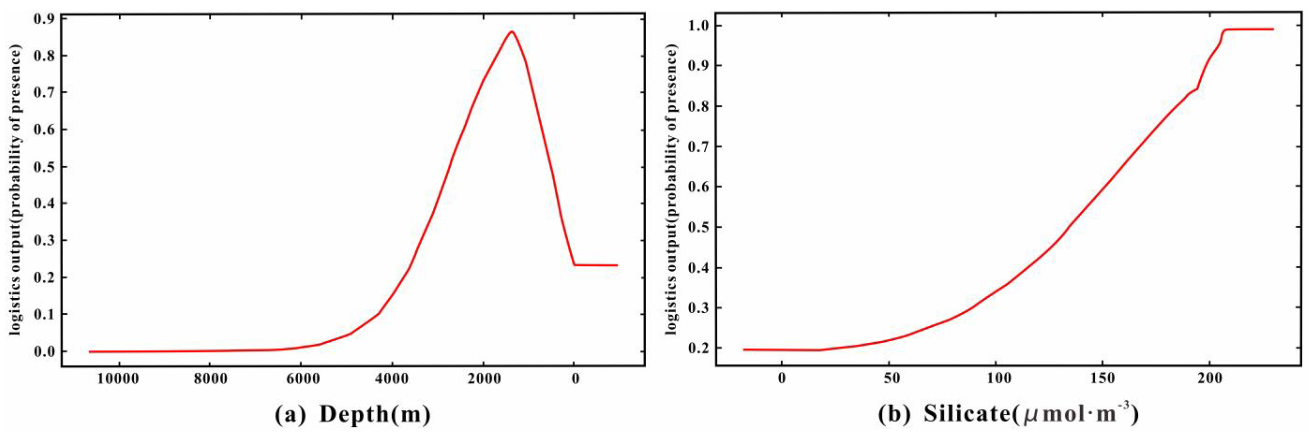
3.2.2. Analysis of Environmental Factors Affecting Species Distribution
4. Discussion
5. Conclusions
Author Contributions
Funding
Institutional Review Board Statement
Informed Consent Statement
Data Availability Statement
Acknowledgments
Conflicts of Interest
| 1 | Available online: https://mapper.obis.org/ (Accessed: 10 March 2023). |
| 2 | Available online: https://www.ncei.noaa.gov/maps/deep-sea-corals/mapSites.htm (Accessed: 13 June 2023). |
| 3 | Available online: https://pangaea.de (Accessed: 19 June 2023). |
References
- Zhonglin, X.; Huanhua, P.; Shouzhang, P. The development and evaluation of species distribution models. Acta Ecol. Sin. 2015, 35, 11. [Google Scholar]
- Hallgren, W.; Santana, F.; Low-Choy, S.; Zhao, Y.; Mackey, B. Species distribution models can be highly sensitive to algorithm configuration. Ecol. Model. 2019, 408, 108719. [Google Scholar] [CrossRef]
- Valavi, R.; Guillera-Arroita, G.; Lahoz-Monfort, J.J.; Elith, J. Predictive performance of presence-only species distribution models: A benchmark study with reproducible code. Ecol. Monogr. 2022, 92, e01486. [Google Scholar] [CrossRef]
- Melomerino, S.M.; Fath, B.D. Ecological niche models and species distribution models in marine environments: A literature review and spatial analysis of evidence. Ecol. Model. 2020, 415, 108837. [Google Scholar] [CrossRef]
- Vohsen, S.A. The Chemical and Microbial Ecology of Deep-Sea Corals; The Pennsylvania State University: State College, PA, USA, 2019. [Google Scholar]
- Quintanilla, E.; Rodrigues, C.F.; Henriques, I.; Hilário, A. Microbial Associations of Abyssal Gorgonians and Anemones (>4000 m Depth) at the Clarion-Clipperton Fracture Zone. Front. Microbiol. 2022, 13, 828469. [Google Scholar] [CrossRef]
- Long, S.; Sparrow-Scinocca, B.; Blicher, M.E.; Arboe, N.H.; Fuhrmann, M.; Kemp, K.M.; Nygaard, R.; Zinglersen, K.; Yesson, C. Identification of a Soft Coral Garden Candidate Vulnerable Marine Ecosystem (VME) Using Video Imagery, Davis Strait, West Greenland. Front. Mar. Sci. 2020, 7, 460. [Google Scholar] [CrossRef]
- Wagner, D.; Friedlander, A.; Pyle, R.L.; Wilhelm, T. Coral Reefs of the High Seas: Hidden Biodiversity Hotspots in Need of Protection. Front. Mar. Sci. 2020, 7, 776. [Google Scholar] [CrossRef]
- Jorgensen, L.L.; Ljubin, P.; Skjoldal, H.R.; Ingvaldsen, R.B.; Anisimova, N.; Manushin, I. Distribution of benthic megafauna in the Barents Sea: Baseline for an ecosystem approach to management. Ices J. Mar. Sci. 2015, 72, 595–613. [Google Scholar] [CrossRef]
- Tong, R.; Purser, A.; Guinan, J.; Unnithan, V.; Yu, J.; Zhang, C. Quantifying relationships between abundances of cold-water coral Lophelia pertusa and terrain features: A case study on the Norwegian margin. Cont. Shelf Res. A Companion J. Deep-Sea Res. Prog. Oceanogr. 2016, 116, 13–26. [Google Scholar] [CrossRef]
- Buhl-Mortensen, L.; Serigstad, B.; Buhl-Mortensen, P.; Olsen, M.N.; Ostrowski, M.; Błażewicz-Paszkowycz, M.; Appoh, E. First observations of the structure and megafaunal community of a large Lophelia reef on the Ghanaian shelf (the Gulf of Guinea). Deep-Sea Res. Part II Top. Stud. Oceanogr. 2017, 137, 148–156. [Google Scholar] [CrossRef]
- Phillips, S.J.; Anderson, R.P.; Schapire, R.E. Maximum entropy modeling of species geographic distributions. Ecol. Model. 2006, 190, 231–259. [Google Scholar] [CrossRef]
- Breiman, L. Random forests, machine learning 45. J. Clin. Microbiol. 2001, 2, 199–228. [Google Scholar]
- Lek, S.; Guégan, J.-F. Artificial Neuronal Networks. In Environmental Science; Springer Science & Business Media: Berlin/Heidelberg, Germany, 2000. [Google Scholar]
- Chen, T.; Guestrin, C. XGBoost: A Scalable Tree Boosting System. In Proceedings of the 22nd ACM Sigkdd International Conference on Knowledge Discovery and Data Mining, San Francisco, CA, USA, 13–17 August 2016. [Google Scholar]
- Assis, J.; Tyberghein, L.; Bosch, S.; Verbruggen, H.; Serrao, E.A.; De Clerck, O. Bio-ORACLE v2.0: Extending marine data layers for bioclimatic modelling. Glob. Ecol. Biogeogr. 2018, 27, 277–284. [Google Scholar] [CrossRef]
- Tozer, B.; Sandwell, D.T.; Smith, W.H.F.; Olson, C.; Beale, J.R.; Wessel, P. Global Bathymetry and Topography at 15 Arc Sec: SRTM15+. Earth Space Sci. 2019, 6, 1847–1864. [Google Scholar] [CrossRef]
- Davies, A.J.; Guinotte, J.M. Global Habitat Suitability for Framework-Forming Cold-Water Corals. PLoS ONE 2011, 6, e18483. [Google Scholar] [CrossRef] [PubMed]
- Steinacher, M.; Joos, F.; Frölicher, T.L.; Plattner, G.K.; Doney, S.C. Imminent ocean acidification in the Arctic projected with the NCAR global coupled carbon cycle-climate model. Biogeosciences 2009, 6, 515–533. [Google Scholar] [CrossRef]
- Cutler, D.R.; Jr, E.T.; Beard, K.H.; Cutler, A.; Hess, K.T.; Gibson, J.; Lawler, J.J. Random forests for classification in ecology. Ecol. A Publ. Ecol. Soc. Am. 2007, 88, 2783–2792. [Google Scholar] [CrossRef] [PubMed]
- Elith, J.; Leathwick, J.R. Species Distribution Models: Ecological Explanation and Prediction Across Space and Time. Annu. Rev. Ecol. Evol. Syst. 2009, 40, 677–697. [Google Scholar] [CrossRef]
- Vignali, S.; Barras, A.G.; Arlettaz, R.; Braunisch, V. SDMtune: An R package to tune and evaluate species distribution models. Ecol. Evol. 2020, 10, 11488–11506. [Google Scholar] [CrossRef]
- Dullo, W.C.; Flögel, S.; Rüggeberg, A. Cold-water coral growth in relation to the hydrography of the Celtic and Nordic European continental margin. Mar. Ecol. Prog. 2008, 371, 165–176. [Google Scholar] [CrossRef]
- Xia, Y.; Liu, C.; Li, Y.; Liu, N. A boosted decision tree approach using Bayesian hyper-parameter optimization for credit scoring. Expert Syst. Appl. 2017, 78, 225–241. [Google Scholar] [CrossRef]
- Allouche, O.; Tsoar, A.; Kadmon, R. Assessing the accuracy of species distribution models: Prevalence, kappa and the true skill statistic (TSS). J. Appl. Ecol. 2006, 43, 1223–1232. [Google Scholar] [CrossRef]
- Thuiller, W.; Lafourcade, B.; Engler, R.; Araújo, M.B. BIOMOD—A platform for ensemble forecasting of species distributions. Ecography 2009, 32, 369–373. [Google Scholar] [CrossRef]
- Breiner, F.T.; Nobis, M.P.; Bergamini, A.; Guisan, A. Optimizing ensembles of small models for predicting the distribution of species with few occurrences. Methods Ecol. Evol. 2018, 9, 802–808. [Google Scholar] [CrossRef]
- Ingram, M.; Vukcevic, D.; Golding, N. Multi-output Gaussian processes for species distribution modelling. Methods Ecol. Evol. 2020, 11, 1587–1598. [Google Scholar] [CrossRef]
- Marchetto, E.; Da Re, D.; Tordoni, E.; Bazzichetto, M.; Zannini, P.; Celebrin, S.; Chieffallo, L.; Malavasi, M.; Rocchini, D. Testing the effect of sample prevalence and sampling methods on probability-and favourability-based SDMs. Ecol. Model. 2023, 477, 110248. [Google Scholar] [CrossRef]
- Marmion, M.; Luoto, M.; Heikkinen, R.K.; Thuiller, W. The performance of state-of-the-art modelling techniques depends on geographical distribution of species. Ecol. Model. 2009, 220, 3512–3520. [Google Scholar] [CrossRef]
- Godsoe, W.; Harmon, L.J. How do species interactions affect species distribution models? Ecography 2012, 35, 811–820. [Google Scholar] [CrossRef]
- Kinlan, B.P.; Poti, M.; Drohan, A.F.; Packer, D.B.; Dorfman, D.S.; Nizinski, M.S. Predictive modeling of suitable habitat for deep-sea corals offshore the Northeast United States. Deep Sea Res. Part I Oceanogr. Res. Pap. 2020, 158, 103229. [Google Scholar] [CrossRef]
- Doherty, B.; Cox, S.P.; Rooper, C.N.; Johnson, S.D.; Kronlund, A.R. Species distribution models for deep-water coral habitats that account for spatial uncertainty in trap-camera fishery data. Mar. Ecol. Prog. Ser. 2021, 660, 69–93. [Google Scholar] [CrossRef]
- Chu, J.W.; Nephin, J.; Georgian, S.; Knudby, A.; Rooper, C.; Gale, K.S. Modelling the environmental niche space and distributions of cold-water corals and sponges in the Canadian northeast Pacific Ocean. Deep Sea Res. Part I Oceanogr. Res. Pap. 2019, 151, 103063. [Google Scholar] [CrossRef]
- Yu, H.; Cooper, A.R.; Infante, D.M. Improving species distribution model predictive accuracy using species abundance: Application with boosted regression trees. Ecol. Model. 2020, 432, 109202. [Google Scholar] [CrossRef]
- Georgian, S.E.; Shedd, W.; Cordes, E.E. High-resolution ecological niche modelling of the cold-water coral Lophelia pertusa in the Gulf of Mexico. Mar. Ecol. Prog. Ser. 2014, 506, 145–161. [Google Scholar] [CrossRef]
- Yesson, C.; Taylor, M.L.; Tittensor, D.P.; Davies, A.J.; Guinotte, J.; Baco, A.; Black, J.; Hall-Spencer, J.M.; Rogers, A.D. Global habitat suitability of cold-water octocorals. J. Biogeogr. 2012, 39, 1278–1292. [Google Scholar] [CrossRef]
- Rathore, M.K.; Sharma, L.K. Efficacy of species distribution models (SDMs) for ecological realms to ascertain biological conservation and practices. Biodivers. Conserv. 2023, 32, 3053–3087. [Google Scholar] [CrossRef]


| Source | Variable Name | Unit | Data Collection Period |
|---|---|---|---|
| Bio-ORACLE v2.0 | Temperature | °C | 2000–2014 |
| Salinity | PSS | 2000–2014 | |
| Silicate | μmol·m−3 | 2000–2014 | |
| Phosphate | μmol·m−3 | 2000–2014 | |
| Nitrate | μmol·m−3 | 2000–2014 | |
| Dissolved Molecular | μmol·m−3 | 2000–2014 | |
| Dissolved Iron | μmol·m−3 | 2000–2014 | |
| Phytoplankton | μmol·m−3 | 2000–2014 | |
| Chlorophyll | mg·m−3 | 2000–2014 | |
| Primary Productivity | g·m−3·day−1 | 2000–2014 | |
| Current Velocity | m·s−1 | 2000–2014 | |
| Satellite Geodesy | Depth | m | 1903–2019 |
| Slope | ° | 1903–2019 | |
| Slope Direction | ° | 1903–2019 | |
| Slope Direction-East | 1 | 1903–2019 | |
| Slope Direction-North | 1 | 1903–2019 | |
| Slope Of Aspect | 1 | 1903–2019 | |
| Slope Of Slope | 1 | 1903–2019 | |
| Ground Roughness | 1 | 1903–2019 | |
| Davies and Guinotte | Vgpm | mg·m−3·d−1 | 2002–2007 |
| Steinacher | Calcite | ΩARAG | 2003–2018 |
| Evaluation Criteria | Bad | General | Favorable | Fabulous |
|---|---|---|---|---|
| AUC | 0.5~0.7 | 0.7~0.8 | 0.8~0.9 | 0.9~1.0 |
| TSS | 0.5~0.6 | 0.6~0.7 | 0.7~0.9 | 0.9~1.0 |
| Kappa | 0.5~0.6 | 0.6~0.7 | 0.7~0.9 | 0.9~1.0 |
| Model | AUC | TSS | KAPPA | TIME(s) |
|---|---|---|---|---|
| Maxent | 0.957 | 0.852 | 0.864 | 670 |
| RF | 0.994 | 0.984 | 0.962 | 3930 |
| ANN | 0.926 | 0.837 | 0.723 | 2508 |
| XGBoost | 0.964 | 0.887 | 0.897 | 2888 |
| Habitability Class | Projected Value |
|---|---|
| Optimum Distribution Area | 0.762 < P < 1.000 |
| More Suitable Distribution Area | 0.409 < P < 0.762 |
| Low-Suitability Distribution Area | 0.119 < P < 0.409 |
| Unsuitable Distribution Area | 0.000 < P < 0.119 |
Disclaimer/Publisher’s Note: The statements, opinions and data contained in all publications are solely those of the individual author(s) and contributor(s) and not of MDPI and/or the editor(s). MDPI and/or the editor(s) disclaim responsibility for any injury to people or property resulting from any ideas, methods, instructions or products referred to in the content. |
© 2024 by the authors. Licensee MDPI, Basel, Switzerland. This article is an open access article distributed under the terms and conditions of the Creative Commons Attribution (CC BY) license (https://creativecommons.org/licenses/by/4.0/).
Share and Cite
Dong, M.; Yang, J.; Fu, Y.; Fu, T.; Zhao, Q.; Zhang, X.; Xu, Q.; Zhang, W. Distribution of Suitable Habitats for Soft Corals (Alcyonacea) Based on Machine Learning. J. Mar. Sci. Eng. 2024, 12, 242. https://doi.org/10.3390/jmse12020242
Dong M, Yang J, Fu Y, Fu T, Zhao Q, Zhang X, Xu Q, Zhang W. Distribution of Suitable Habitats for Soft Corals (Alcyonacea) Based on Machine Learning. Journal of Marine Science and Engineering. 2024; 12(2):242. https://doi.org/10.3390/jmse12020242
Chicago/Turabian StyleDong, Minxing, Jichao Yang, Yushan Fu, Tengfei Fu, Qing Zhao, Xuelei Zhang, Qinzeng Xu, and Wenquan Zhang. 2024. "Distribution of Suitable Habitats for Soft Corals (Alcyonacea) Based on Machine Learning" Journal of Marine Science and Engineering 12, no. 2: 242. https://doi.org/10.3390/jmse12020242
APA StyleDong, M., Yang, J., Fu, Y., Fu, T., Zhao, Q., Zhang, X., Xu, Q., & Zhang, W. (2024). Distribution of Suitable Habitats for Soft Corals (Alcyonacea) Based on Machine Learning. Journal of Marine Science and Engineering, 12(2), 242. https://doi.org/10.3390/jmse12020242