Abstract
Constantly growing environmental concerns focused on reducing pollution, in addition to rising fuel costs in recent years, have led the maritime industry to develop and implement fuel-saving solutions. Among them is the optimization of marine propeller efficiency, as marine propellers are a crucial part of ship’s propulsion system. During the initial design stage, selecting the optimal propeller is considered a multi-objective optimization process. This research focused on maximizing propeller open water efficiency, while minimizing engine brake power constrained by thrust and cavitation. Optimization was applied to Wageningen B-series propellers and conducted using the Non-Dominated Sorting Genetic Algorithm II (NSGA-II). The algorithm selected optimum parameters to create the propeller model, which was then evaluated numerically through computational fluid dynamics (CFD) with a multiple reference frame (MRF) and under the SST k-ω turbulence model, to obtain the open water hydrodynamic characteristics. In addition, the cavitation effect was evaluated using the Zwart–Gerber–Belamri cavitation model. The numerical model results were validated through comparison with open water experimental data from the Netherlands Ship Model Basin for the Wageningen B-series propellers. The results showed errors of 3.29% and 2.01% in efficiency under noncavitating and cavitating conditions, respectively. Correct performance of the functions was shown, based on neural networks trained to estimate thrust and torque coefficients instead of polynomials. The proposed optimization process and numerical model are suitable for solving multi-objective optimization problems in the preliminary design of fixed-pitch marine propellers.
1. Introduction
The primary goal of marine propeller design is to achieve the highest level of propulsive efficiency. Higher propeller efficiency impacts positively on fuel consumption, decreasing operational costs. Constantly increasing oil prices, in addition to stringent regulations imposed on ships concerning air pollution and restrictions on NOX and SOX emissions, have led the shipping industry to further develop efficient propellers [1,2,3,4]. On the other hand, in order to prevent vibration and sound issues in the hull, it is important to avoid cavitation, despite this being a common occurrence in almost all ship propellers [5,6]. Thus, it is crucial to maintain low cavitation levels from the initial design phase. Designers often face a complex task in balancing efficiency and cavitation [7].
Cavitation occurs when the local pressure drops below the vapor pressure of the liquid at the corresponding temperature. Propeller blades are exposed to local lift forces that can lead to low-pressure peaks. When the surrounding water pressure drops below the vapor pressure, cavities or bubbles will form. Because of their specific geometry and the rotational conditions in which marine propellers operate, cavitation is likely to occur [8,9]. Cavitation phenomena, when present, can lead to safety problems, major repair and maintenance costs, and additional hydrodynamic energy losses [7,10].
Wageningen B-series propellers [11] have one of the largest and most common datasets available, as a result of experimental data. Propellers analyzed in this series provide parameterization, in order to be able to select a specific propeller among a continuous set of combinations that are valid when properly bounded [12]. In order to estimate a ship’s required power and achieve the designed speed and thrust, certain parameters and hydrodynamic characteristics must be matched. These selected parameters include four geometric and one operational parameter: propeller diameter (D), pitch ratio (P/D), expanded area ratio (AE/A0), propeller blade number (Z), and propeller rotational speed (n) [13,14]. The hydrodynamic characteristics are the dimensionless coefficients: thrust coefficient (KT), torque coefficient (KQ), and open water efficiency (ηO). In the conceptual design stage, optimization of the propeller is complex, due to the number of variables and constraints involved, resulting in a multi-objective problem [15]. There is no unique solution, as one solution may be better for one objective but not for others [7].
Since the Wageningen B-series propeller dataset has existed, it has formed the basis for a large number of studies, given it provides the experimental data required to validate any theory or mathematical model related to phenomena occurring in a propeller.
Genetic algorithms (GA) are part of the family of heuristic optimization methods useful for performing optimizations for either single or multi-objective problems. GAs have been applied in the marine industry for solving a variety of problems related to propellers. Lee and Lin [16] implemented a GA to determine the stacking sequence needed to fabricate a composite propeller useful at a wide range of speeds. Pluciński et al. [17] studied the design of a self-twisting composite propeller with an efficiency optimized for a variety of inflow velocities, using a GA to determine the orientation angles for the fiber in each layer. Gypa et al. [18] used an interactive GA and machine learning approach to optimize the parameters of a propeller based on cavitation constraints; for this purpose, the authors used a vortex lattice method for hydrodynamic evaluation. Ebrahimi et al. [19] carried out a study by applying GA to optimize a baseline propeller, in order to reduce propeller noise, while maximizing hydrodynamic efficiency. They performed experimental tests and validated their results using the Ffowcs Williams–Hawkings (FW-H) model compared to noise measurements.
GAs applied to the Wageningen B-series propellers have focused on addressing single-objective or multi-objective optimizations, considering a variety of goals and constraints. Optimization, in most cases, is not shown as a validated process, as the purpose is only to show the behavior and convergence of optimization. Chen and Shih [20] used a GA to optimize the design of a B-series propeller, considering vibration and efficiency as objective functions. Xie [15] implemented the Non-Dominated Sorting Genetic Algorithm II (NSGA-II) to maximize the propeller efficiency and thrust coefficient at a single design speed for a B-series propeller. Esmailian et al. [21] proposed a methodology to optimize the hull-propeller system of a Series-60 ship equipped with a B-series propeller, using NSGA-II with two objective functions given by lifetime fuel consumption (LFC) and a cost function including several propeller parameters. Permadi and Sugianto [14] applied NSGA-II to obtain parameters of three-bladed and five-bladed B-series propellers, in order to optimize thrust and open water efficiency, subject to a thrust constraint. Huisman and Foeth [22] applied NSGA-II to optimize the parametric propeller geometries of two propellers under two case studies, to maximize efficiency under different constraints and minimize cavitation. This study is of great relevance, given it was conducted by the Maritime Research Institute Netherlands (MARIN), who created the original Wageningen B-Series propeller database at the Netherlands Ship Model Basin.
The present study aimed to investigate the advantages of using the NSGA-II genetic algorithm to optimize the preliminary design of a Wageningen B-series propeller. The objectives were to maximize open water efficiency, while minimizing brake power and inherent fuel consumption, with cavitation and thrust coefficient as the constraints. Convergence of the GA determined the geometry and characteristics of the propeller as follows: J = 0.73, P/D = 1.1049, AE/A0 = 0.5823, ηO = 0.6363, Z= 5, n = 368 rpm, and PB = 2765 kW. The hydrodynamic characteristics in open water and in cavitation conditions were studied using CFD. Subsequently, validation of the results against experimental data from the Wageningen B-series was performed.
2. Theory and Methods
2.1. Description of the Multi-Objective Optimization Design Process
The overall process for the multi-objective optimization design and validation of a Wageningen B-series propeller is described in Figure 1.
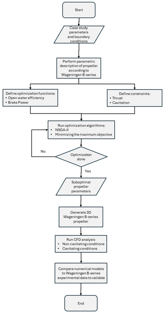
Figure 1.
Flowchart of the multi-objective optimization and validation process.
The available data and boundary conditions used to perform this study are given by a case study of an offshore patrol vessel (OPV). A parametric description of the Wageningen B-series propellers is used, given their dataset is publicly available to perform validation of any numerical model. This was a multi-objective study as it was necessary to optimize two functions; open water efficiency was maximized, while power brake was minimized. Constraints for optimization were given as achieving the required thrust while avoiding cavitation. Optimization was based on the NSGA-II algorithm; however, for comparison, a variation of the goal attainment method called minimizing the maximum objective was used, which is also suitable for multi-objective optimization. Both algorithms were implemented, and their results were presented, in order to select the best suboptimal set of parameters to describe the Wageningen B-series propeller, which were then drawn and used to run numerical models in both cavitation and non-cavitation conditions. The final results were compared to experimental data to validate the optimization and numerical model.
2.2. Case Study
In order to apply our research methodology, a twin-screw offshore patrol vessel (OPV) was used, as shown in Figure 2, and its main characteristics can be found in Table 1. For the purposes of optimization, the propeller diameter was kept constant. The total resistance was obtained through performing an analysis with the Holtrop method at cruising speed, i.e., RT = 163,040.37 N.
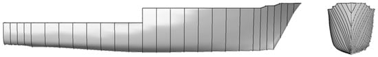
Figure 2.
OPV hull.

Table 1.
OPV main characteristics.
2.3. Wageningen B-Series Propellers
Systematic propeller series based on experimental data from open water model tests are commonly used in the early design stage to determine the optimal geometric parameters. The systematic series used in this project was the common Wageningen B-series. The B-series was first developed by Troost [23,24,25], and later improvements were published by Lammeren et al. [11]. Subsequently, Oosterveld and Oossanen [26] fitted the KT-KQ data and presented them as regression polynomials, shown in Equations (1) and (2). An alternative approach to computing KT and KQ coefficients based on neural networks is presented in Section 5.3.
Usually, open water test characteristics are presented in dimensionless form and plotted in terms of KT, KQ, and ηO on a J-basis [8]. Their respective equations are as follows:
2.4. Cavitarion Criteria
Blade preliminary design can be performed using one of the basic procedures such as a Burrill cavitation table or Keller’s equation. Keller formulated an equation for obtaining an early estimate of the required expanded area ratio (EAR). This equation provides the minimum required EAR, as shown in Equation (7) [13,27].
In Equation (7), represents the thrust required at the designed speed; is the absolute pressure located at the shaft’s center given by the atmospheric pressure plus the hydrostatic pressure ; is the vapor pressure given by 0−3 MPa at °C according to ITTC; is the propeller diameter; and is a constant given by
for single propeller ships.
for twin propeller ships.
Depth for propeller shaft’s center can be estimated from Equation (8).
The start of cavitation can be estimated using CFD and analyzing cavitation number by means of the local pressure at the propeller surface. In this sense, it is necessary to model the phase transition [8]. One of the goals during the design stage of hydrodynamic systems is to avoid or at least delay cavitation phenomena. The cavitation number is used as an index to quantify the probability of cavitation occurring [13]. Helal et al. [9] described the beginning of cavitation phenomena as cavitation inception. Cavitation number and pressure coefficient are defined in Equations (9) and (10); and if inequality occurs, then cavitation begins. The higher the cavitation number, the lower the probability cavitation forming [13].
2.5. Non-Dominated Sorting Genetic Algorithm-II (NSGA-II)
The genetic algorithm (GA) was created by Holland [28], and it was inspired by Darwin’s biological evolution theory. In the beginning, a GA creates a set of chromosomes, which are random initial populations. Then, genetic operators such as selection, crossover, and mutation are used to produce a new generation [29]. As each generation passes, the population produces increasingly fit individuals. This process eventually stops after a certain number of generations. During this process, the fittest individual overall, which represents the global optimum, is identified [17].
In particular cases, it is necessary to address a problem with more than one objective function, which leads to a multi-objective optimization problem. NSGA-II is one of the most widely used and generalized methods for solving multi-objective problems. It was proposed by Deb et al. [30] and it introduces the concept of elitism, to improve its convergence properties [31]. NSGA-II is an elitist GA that prioritizes individuals with better fitness values and that can increase the population diversity, even if their fitness value is lower.
Figure 3 presents a flowchart of the general process of NSGA-II. The algorithm begins by creating a random population of solutions named generation 1. The second step is evaluating the fitness functions of the population using corresponding optimization constraints; the results are classified into nondominated layers named Pareto fronts with an assigned rank. The upper layer contains the nondominated or nonsurpassed solutions. In order to enhance the diversity among the population and prevent early convergence, a crowding distance is computed and assigned to each solution. Prioritizing low nondominated ranks with higher crowding distances, selection is performed using tournaments to find the best adapted individuals. Further operations are applied to selected individuals, such as crossover and mutation, with the goal of creating new child solutions. Elitist selection is applied in order to select the best individuals from the current population and pass them unaltered to the next generation. The process of selection, crossover, mutation, and elitism keeps repeating until the convergence criteria or the maximum number of generations is reached.
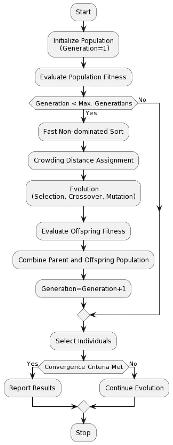
Figure 3.
Flowchart of the general NSGA-II process.
According to Akbari et al. [32], in a Pareto front set of solutions, at least one solution is inferior to another, even though the set as a whole is better than other solutions in the remaining search space. Nevertheless, according to Kramer [33], GAs are excellent for optimizing difficult problems where classical methods fail due to their complexity.
3. Propeller Optimization
3.1. Multi-Objective Optimization Algorithms
The first objective function was used to maximize the open water efficiency, as seen in Equation (11), from polynomials KT and KQ, in Equations (1) and (2), respectively. The second objective function helps the ship attain cruise speed with the minimum amount of power delivered to the propeller (PD) and brake power (PB) supplied by the engines. Assuming that there is no friction or transmission losses (ηS = 1), the second objective function to be minimized is defined in Equation (12).
Two explicit constraints are used for optimization. The first is related to Keller’s cavitation criterion [27,34] and can be expressed as the nonlinear inequality shown in Equation (13). The second constraint is the required thrust (T), which is based on the definition of the thrust coefficient (KT); therefore, a nonlinear equality as expressed in Equation (14) was established.
Both functions and constraints were implemented in MATLAB® R2023b software for the NSGA-II, and the minimizing the maximum objective algorithms used the “gamultiobj” and the “fminimax” functions, respectively. The parameters used to run the gamultiobj function are presented in Table 2, while the parameters needed to initialize and run the fminimax function are shown in Table 3.
Table 2.
Configuration parameters for the NSGA-II.
Table 3.
Configuration parameters for the minimizing the maximum objective algorithms.
Table 4 summarizes the limits for the variables and search space for optimization. The standard range characteristics of the B-series are represented by the limits of J, P/D, and AE/A0, whereas n covers a reasonable design range and D remains a fixed variable.
Table 4.
Search space.
During execution of the code, the number of blades (Z) was varied between 4 and 5, to cover the most common commercial range. Table 5 presents a comparison of the results obtained from the algorithms for each number of blades. It was observed that the best results were obtained with the NSGA-II algorithm for Z = 5; therefore, this number was used to construct the 3D geometry of the propeller.
Table 5.
Suboptimal parameters obtained using gamultiobj and fminimax.
3.2. Geometric Model
The propeller geometry was obtained from the table of general geometric properties for the B-series, as well as equations from Oosterveld and Van Oossanen [26]. Using a standardized parametric propeller series, such as the B-series, has an enormous advantage, as foils to form the blade sections can be generated with coordinates, as depicted in Figure 4. After computing the blade section coordinates, they were exported to create the 3D geometry shown in Figure 5a. Based on the hydrodynamic terms of ITTC [35], the global Cartesian coordinate system (X, Y, Z) of the propeller was defined as outlined in Figure 5b. When looking from aft (−X), a positive rotational speed indicates clockwise rotation and a negative speed indicates counterclockwise rotation, following the right-hand rule.
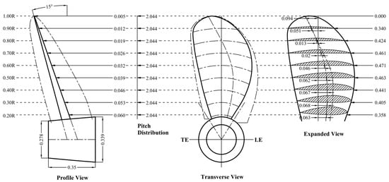
Figure 4.
Propeller coordinates obtained for Z = 5.
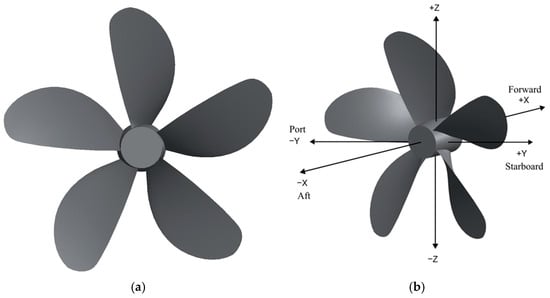
Figure 5.
(a) Propeller model in 3D; (b) global coordinate system.
4. Numerical Model
4.1. Computational Domain
The computational domain of the study used a multiple reference frame (MRF), also known as the frozen rotor approach, as shown in Figure 6. The static or frozen domain was 3 diameters wide and 10 diameters long, to allow open fluid development after it accelerates through the propeller. The rotor, which is situated near the propeller, had a width of 0.38 diameters and a height of 1.2 diameters. Considering the size of the rotor domain is crucial, as it impacts the computational cost. If the domain is too large, this will increase the cost; on the other hand, if it is too small, this will result in the formation of large eddies near the propeller, leading to imprecise results. Meanwhile, the “rotor” subdomain was assigned an angular rotational speed n, subject to the advance coefficient J. In the “frozen” domain, a static condition was assigned. According to the MRF approach methodology [36], the interface zone between subdomains was also specified.
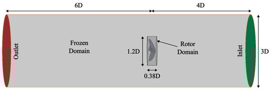
Figure 6.
MRF computational domain.
4.2. Governing Equations
Research on turbo-machinery, aircraft propellers, and ship propellers is focused on studying rotational motion. A practical method of representation is using the multiple reference frame (MRF) approach [36], where the geometric model includes a rotational component with respect to a fixed reference. Transitory phenomena are explained through separating the fluid domain into subdomains with at least one fixed subdomain, one rotational subdomain, and interfaces among them.
MRF uses stationary approximations of the transitory rotation at an instant of time. Flow rotation around moving parts is simulated, adding Coriolis source terms and centripetal accelerations to the momentum equation. The flow in fixed subdomains is governed by continuity and momentum equations (Equations (15) and (16)); meanwhile, the rotational subdomains are governed by continuity and momentum equations for the MRF, as seen in Equations (17) and (18).
Equations for the MRF can be expressed using relative or absolute velocities as dependent variables [37]. Pressure-based solvers from ANSYS® Fluent can be configured to use any of those two options. This numerical model was implemented using the absolute velocity.
4.3. Turbulence Model
Reynolds-averaged Navier–Stokes (RANS) turbulence models are a set of two transport equation turbulence models. The turbulence model is an empiric model containing the turbulent kinetic energy (k) and the turbulent dissipation frequency (w) that was developed by Wilcox [38]. The turbulence model has been improved over time; this is the case of the shear stress transport (SST) turbulence model developed by Menter [39]. It adds a laminar boundary layer model that includes a mix function to be applied to the and the boundary layer models, to give different responses near the wall and in the freestream depending on the value of the function.
Even though there are several turbulence models that can be applied to model phenomena happening at the boundary layer, this research used the SST turbulence model, as the aforementioned features make it one of the most widely used turbulence models in CFD simulations related to aerodynamics and hydrodynamics, as it provides good results for flows with strong pressure gradients and flow separation for surfaces with curvatures [37]. The SST turbulence model is expressed in Equations (19) and (20).
4.4. Multiphase Model
As described by Helal et al. [9], flow under cavitation is a two-phase mix made of vapor and liquid that is simplified and simulated as a mix of a single phase. Considering an homogeneous mix, multiphase flow can be solved using modified RANS equations. The continuity and momentum for the mix are described in Equations (21) and (22).
In the multiphase approach, density and viscosity are represented as a volume fraction of the secondary phase, as expressed in Equations (23) and (24), respectively. The liquid–vapor mass transport is governed by the vapor transport in Equation (25). Likewise, the mass transfer between fluid and bubbles is modeled using a derivation of the generalized Rayleigh–Plesset equation, as shown in Equation (26).
Bubble formation was applied to the numerical model in ANSYS® Fluent, using the Zwart–Gerber–Belamri cavitation model from Zwart et al. [40]. This cavitation model assumes all bubbles have the same size and is expressed in Equations (27) and (28).
4.5. CFD Configuration and Boundary Conditions
Table 6 summarizes the boundary conditions for each variation in J applied to the rotating domain. At the inlet, the flow was homogeneous at a constant advance velocity of 8.276 m/s. The flow went downstream from bow to stern, with a turbulence intensity of 1%. The static domain of the outer walls were subjected to symmetry conditions, while the propeller walls were established using a no-slip condition.
Table 6.
Simulated boundary conditions.
For CFD analysis, two configurations were used to perform different simulations: a noncavitating simulation, and a cavitation behavior simulation. The former was conducted at various advance coefficients J, as previously listed in Table 5. The latter was performed at the optimal operating conditions (Case II). Both configurations involved the use of a C-mesh. The freshwater properties were obtained from ITTC [41] data at 25 °C. Table 7 and Table 8 provide a summary of the numerical configurations used.
Table 7.
Solver configuration for noncavitating conditions.
Table 8.
Solver configuration for cavitating conditions.
4.6. Domain Discretization
Three unstructured meshes (A, B, and C) were generated, varying the number of elements between 2.21 × 10⁶ and 9.27 × 10⁶. The tetrahedron method was applied to the complete domain, with a growth factor of 1.2. In the critical region near the propeller walls, the inflation technique was applied to increase the resolution and better represent the boundary layer, as shown in Figure 7 and Figure 8.
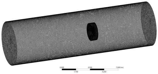
Figure 7.
MRF fluid domain.
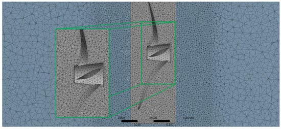
Figure 8.
Interface of frozen and rotational subdomains.
A mesh sensitivity study was conducted to estimate the balance between computational cost and mesh density, obtaining results with a good correlation compared with the experimental data, thus ensuring mesh independence. Metrics for seven meshes were analyzed, in order to meet the criteria established by ANSYS® Inc. (Canonsburg, PA, USA). [42] of having a good mesh quality, as observed in Table 9. The numerical model was run with every mesh using fresh water in noncavitating conditions (Case II) to calculate the thrust (T), torque (Q), and corresponding open water efficiency (ηO). The results were then compared against experimental B-series data, as presented in Table 10.
Table 9.
Mesh metrics.
Table 10.
Mesh sensibility analysis.
The plots in Figure 9, Figure 10 and Figure 11 show the convergence of the thrust, torque, and open water efficiency in the numerical model as the number of elements/nodes was increased to discretize fluid domains using the finite volume method (FMV). As the number of elements/nodes was increased, the convergence of the results in order to make them mesh independent became evident. The mesh selected for the study was mesh F, as it resulted in the first point of the convergence curve after the values had settled.
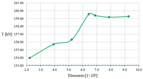
Figure 9.
Mesh sensitivity plot for thrust.
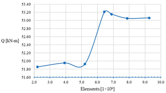
Figure 10.
Mesh sensitivity plot for torque.
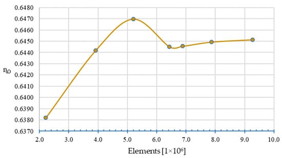
Figure 11.
Mesh sensitivity plot for open water efficiency.
5. Results
5.1. Noncavitating Condition
Table 11 and Figure 12 and Figure 13 show a comparison between the numerical model results and the B-series experimental data by means of computing the relative error. In general, a good correlation is considered having a maximum error of less than 10%, according to [43]. The highest error percentage was 8.32% in the thrust coefficient, while the highest error in the torque coefficient was 6.23%, both at J = 0.90. In the case of the open water efficiency, this obtained the lowest percentage error of the set, at J = 0.90. Figure 14 and Figure 15 illustrate a comparison of the thrust and torques from the numerical models against the expected values from the experimental data, showing a good correlation, with errors not exceeding 10%.
Table 11.
Results in noncavitating conditions.
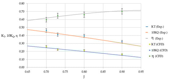
Figure 12.
Propeller characteristics with 5% error bars.
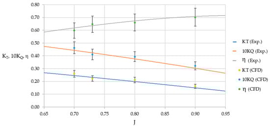
Figure 13.
Propeller characteristics with 10% error bars.
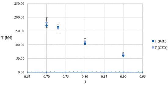
Figure 14.
Propeller thrust with 10% error bars.
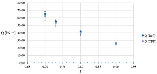
Figure 15.
Propeller torque with 10% error bars.
5.2. Cavitating Condition
This section shows the results obtained from the numerical model implemented considering cavitation; it used a multiphase mixing model and the Zwart–Gerber–Belamri cavitation model. After optimization, J = 0.73 (Case II from Table 5) was the optimal point at which the two objective functions were optimized, as power brake was minimal, while the open water efficiency was the maximum. At the same time, for an optimization that minimizes cavitation as a constraint, the propeller operating point and its characteristics should show minimal or no presence of cavitation. Table 12 shows the results of the numerical model considering cavitation and experimental data from B-series. Likewise, with the noncavitating numerical model, it was observed that the error percentage did not exceed 5%.
Table 12.
Results in cavitating conditions.
The best representation of the occurrence of cavitation is the vapor fraction as a result of the numerical model. The proportion of vapor present in the two-phase mixture is visualized with respect to the liquid phase. A value of 1 or close to this number will show that vapor bubbles are fully formed and cavitation is happening. Figure 16 depicts the different values of vapor volume fraction present on both sides of the optimized propeller. In Figure 16a, a low volume fraction at the propeller tips can be observed, while in Figure 16b a wide range of values for the vapor volume fraction can be observed; this means the suction side is the surface of the propeller with the higher probability of having cavitation. The areas with the cooler shades signify a null or lower vapor fraction, whereas warmer colors signify a higher presence of vapor fraction, or in other words cavitation.
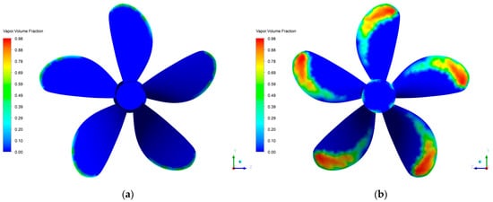
Figure 16.
Vapor volume fraction contour at J = 0.73. (a) Pressure side; (b) suction side.
The development of cavitation was further analyzed. The vapor volume iso-surface of fractions 0.1, 0.5, and 0.90 are presented in Figure 17 and Figure 18. From these Figures, it can be observed that high values of vapor volume fraction, i.e., 0.9 or higher, were present in a minimal portion of the propeller. These contours suggest that if cavitation occurred, it would be of the sheet cavitation type occurring at the suction face.
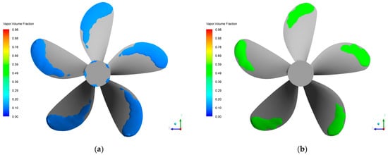
Figure 17.
Details of vapor volume fraction. (a) Volume fraction at 0.1; (b) volume fraction at 0.5.
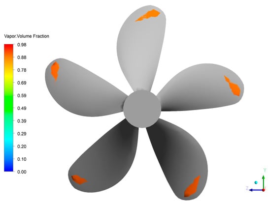
Figure 18.
Details of vapor volume fraction at 0.90.
5.3. Approximation of KT and KQ Coefficients Using Neural Networks
Polynomials for retrieving KT and KQ coefficients for the Wageningen B-series propeller were first introduced by Oosterveld and Oossanen [26]; since then they have been used as the primary means to obtain these values, together with corresponding plots. Comparatively, in a similar way to how polynomials were developed through multiple regressions in order to fit experimental data, nowadays neural networks (NN) can be trained with a set of data points in order to predict the same coefficients. Data from [26,44] were used to train two independent neural networks using MATLAB® with the parameters seen in Table 13. The performance in training neural networks for KT and KQ is shown in Figure 19 and Figure 20, respectively; end of training is marked with the green circle.
Table 13.
Configuration parameters for training the neural networks.
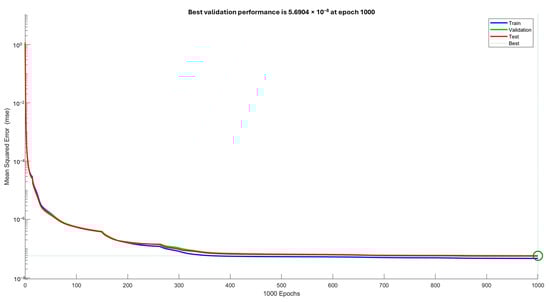
Figure 19.
Performance in training neural network for KT.
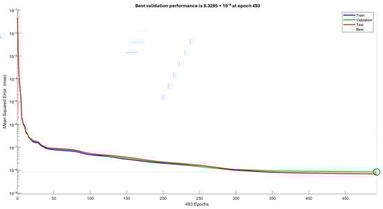
Figure 20.
Performance in training neural network for KQ.
In order to compare the results from using polynomials and neural networks, coefficients and efficiencies were plot corresponding to Wageningen B-series for Z, AE/A0, and P/D using the suboptimal parameters obtained from the NSGA-II algorithm. Figure 21 shows a plot using polynomials, Figure 22 shows a plot using neural networks, and Figure 23 depicts the absolute error between the polynomial and neural network estimations for KT and KQ. From Figure 23, it can be observed that errors fell within a range of 10−4 in this specific case.
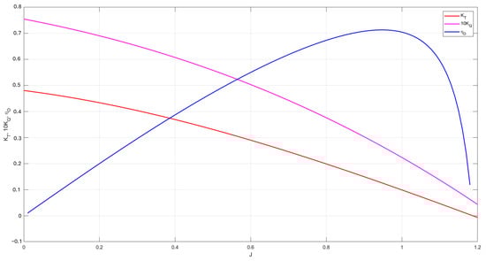
Figure 21.
Wageningen B-series plot with suboptimal parameters using polynomials.
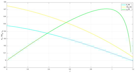
Figure 22.
Wageningen B-series plot with suboptimal parameters using neural networks.
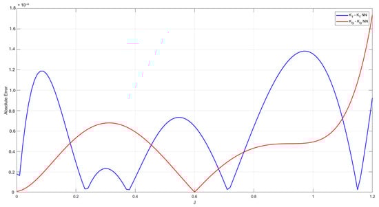
Figure 23.
Error plot for estimations of KT and KQ using polynomials and neural networks.
6. Conclusions
In this research, the benefit of using the NSGA-II genetic algorithm to optimize the preliminary design of a Wageningen B-series propeller was studied. Among the many possible configurations, the algorithm selected one that increased the open water efficiency and minimized the ship brake power within the thrust and cavitation constraints. CFD simulations using the SST k-ω turbulence model and MRF approach allowed the analysis of the hydrodynamic characteristics in noncavitating and cavitation conditions. Based on the numerical results obtained, the following conclusions were reached:
- The numerical model indicated a close correlation between the numerical predictions and experimental data in noncavitating conditions. With maximum errors of 8.32%, 6.23%, and 3.29% for KT, KQ, and ηO, respectively.
- The use of a multiphase approach and the Zwart–Gerber–Belamri cavitation model enabled a detailed investigation into the propeller cavitation phenomenon. The numerical model revealed that the propeller underwent partial cavitation on its suction side, while also revealing a 2.01% error between the efficiency ηO of the numerical model’s operating point and the experimental data.
- Performing mesh refinement, particularly in the areas of interest, such as the tips and leading edge of the blades, could improve the capture of tip and sheet type cavitation effects in future research.
- Functions derived from trained neural networks could be used for estimating KT and KQ coefficients instead of the original polynomials.
The presented methodology was to be feasible for addressing complex and multivariable problems in the field of naval engineering by combining two advanced techniques: genetic algorithm optimization and CFD analysis.
Author Contributions
Conceptualization, A.V.-S., M.E.T.-d.-C., J.H.-H. and N.C.-Z.; methodology, A.V.-S., M.E.T.-d.-C., J.H.-H., A.L.H.-M. and N.C.-Z.; software, A.V.-S. and M.E.T.-d.-C.; validation, A.V.-S., M.E.T.-d.-C., J.H.-H. and N.C.-Z.; formal analysis, A.V.-S., M.E.T.-d.-C., J.H.-H., A.L.H.-M. and N.C.-Z.; investigation, A.V.-S., M.E.T.-d.-C., J.H.-H., A.L.H.-M. and N.C.-Z.; resources, A.V.-S., M.E.T.-d.-C. and N.C.-Z.; data curation, A.V.-S., M.E.T.-d.-C., J.H.-H., A.L.H.-M., N.C.-Z. and L.d.C.S.-C.; writing—original draft preparation, A.V.-S., M.E.T.-d.-C., J.H.-H. and N.C.-Z.; writing—review and editing, M.E.T.-d.-C., J.H.-H. and N.C.-Z.; visualization, M.E.T.-d.-C. and J.H.-H.; supervision, M.E.T.-d.-C., A.L.H.-M. and L.d.C.S.-C.; project administration, M.E.T.-d.-C. and L.d.C.S.-C. All authors have read and agreed to the published version of the manuscript.
Funding
The APC was funded by the Master in Applied Engineering of Universidad Veracruzana.
Data Availability Statement
Data are contained within the article.
Acknowledgments
A.V.-S. extends her gratitude to the Consejo Nacional de Humanidades, Ciencias y Tecnologías for the scholarship granted during her master’s studies.
Conflicts of Interest
The authors declare no conflict of interest. The funders had no role in the design of the study; in the collection, analyses, or interpretation of data; in the writing of the manuscript; or in the decision to publish the results.
References
- Bertetta, D.; Brizzolara, S.; Canepa, E.; Gaggero, S.; Viviani, M. EFD and CFD Characterization of a CLT Propeller. Int. J. Rotating Mach. 2012, 2012, e348939. [Google Scholar] [CrossRef]
- Yusvika, M.; Fajri, A.; Tuswan, T.; Prabowo, A.R.; Hadi, S.; Yaningsih, I.; Muttaqie, T.; Laksono, F.B. Numerical Prediction of Cavitation Phenomena on Marine Vessel: Effect of the Water Environment Profile on the Propulsion Performance. Open Eng. 2022, 12, 293–312. [Google Scholar] [CrossRef]
- Xing, H.; Spence, S.; Chen, H. A Comprehensive Review on Countermeasures for CO2 Emissions from Ships. Renew. Sustain. Energy Rev. 2020, 134, 110222. [Google Scholar] [CrossRef]
- Third IMO GHG Study 2014. Available online: https://www.imo.org/en/ourwork/environment/pages/greenhouse-gas-studies-2014.aspx (accessed on 15 December 2023).
- Gaggero, S.; Rizzo, C.M.; Tani, G.; Viviani, M. EFD and CFD Design and Analysis of a Propeller in Decelerating Duct. Int. J. Rotating Mach. 2012, 2012, e823831. [Google Scholar] [CrossRef]
- Sezen, S.; Atlar, M. Numerical Investigation into the Effects of Tip Vortex Cavitation on Propeller Underwater Radiated Noise (URN) Using a Hybrid CFD Method. Ocean Eng. 2022, 266, 112658. [Google Scholar] [CrossRef]
- Mirjalili, S.; Lewis, A.; Mirjalili, S.A.M. Multi-Objective Optimisation of Marine Propellers. Procedia Comput. Sci. 2015, 51, 2247–2256. [Google Scholar] [CrossRef]
- Molland, A.F.; Turnock, S.R.; Hudson, D.A. Ship Resistance and Propulsion: Practical Estimation of Ship Propulsive Power; Cambridge University Press: Cambridge, UK, 2011; ISBN 978-0-521-76052-2. [Google Scholar]
- Helal, M.; Ahmed, T.; Banawan, A.; Kotb, M. Numerical Prediction of Sheet Cavitation on Marine Propellers Using CFD Simulation with Transition-Sensitive Turbulence Model. AEJ-Alex. Eng. J. 2018, 57, 3805–3815. [Google Scholar] [CrossRef]
- Lee, C.-S.; Choi, Y.-D.; Ahn, B.-K.; Shin, M.-S.; Jang, H.-G. Performance Optimization of Marine Propellers. Int. J. Nav. Archit. Ocean Eng. 2010, 2, 211–216. [Google Scholar] [CrossRef]
- van Lammeren, W.; Manen, J.D.; Oosterveld, M. The Wageningen B-Screw Series; SNAME: New York, NY, USA, 1969; Volume 77, pp. 269–317. [Google Scholar]
- Helma, S. Surprising Behaviour of the Wageningen B-Screw Series Polynomials. J. Mar. Sci. Eng. 2020, 8, 211. [Google Scholar] [CrossRef]
- Birk, L. Fundamentals of Ship Hydrodynamics: Fluid Mechanics, Ship Resistance and Propulsion; John Wiley & Sons: Hoboken, NJ, USA, 2019; ISBN 978-1-118-85548-5. [Google Scholar]
- Permadi, N.V.A.; Sugianto, E. CFD Simulation Model for Optimum Design of B-Series Propeller Using Multiple Reference Frame (MRF). CFD Lett. 2022, 14, 22–39. [Google Scholar] [CrossRef]
- Xie, G. Optimal Preliminary Propeller Design Based on Multi-Objective Optimization Approach. Procedia Eng. 2011, 16, 278–283. [Google Scholar] [CrossRef]
- Lee, Y.-J.; Lin, C.-C. Optimized Design of Composite Propeller. Mech. Adv. Mater. Struct. 2010, 11, 17–30. [Google Scholar] [CrossRef]
- Pluciński, M.M.; Young, Y.L.; Liu, Z. Optimization of a Self-Twisting Composite Marine Propeller Using Genetic Algorithms. In Proceedings of the ICCM International Conferences on Composite Materials, Kyoto, Japan, 8–13 July 2007. [Google Scholar]
- Gypa, I.; Jansson, M.; Wolff, K.; Bensow, R. Propeller Optimization by Interactive Genetic Algorithms and Machine Learning. Ship Technol. Res. 2023, 70, 56–71. [Google Scholar] [CrossRef]
- Ebrahimi, A.; Seif, M.S.; Nouri-Borujerdi, A. Hydro-Acoustic and Hydrodynamic Optimization of a Marine Propeller Using Genetic Algorithm, Boundary Element Method, and FW-H Equations. J. Mar. Sci. Eng. 2019, 7, 321. [Google Scholar] [CrossRef]
- Chen, J.-H.; Shih, Y.-S. Basic Design of a Series Propeller with Vibration Consideration by Genetic Algorithm. J. Mar. Sci. Technol. 2007, 12, 119–129. [Google Scholar] [CrossRef]
- Esmailian, E.; Ghassemi, H.; Zakerdoost, H. Systematic Probabilistic Design Methodology for Simultaneously Optimizing the Ship Hull–Propeller System. Int. J. Nav. Archit. Ocean Eng. 2017, 9, 246–255. [Google Scholar] [CrossRef]
- Huisman, J.; Foeth, E. Automated Multi-Objective Optimization of Ship Propellers; Maritime Research Institute Netherlands (MARIN): Espoo, Finland, 2017. [Google Scholar]
- Troost, L. Open-Water Test Series with Modern Propeller Forms: A Paper Read in a Symposium on Propellers Before the North East Coast Institution of Engineers and Shipbuilders in Newcastle upon Tyne on the 1st April, 1938; North East Coast Institution of Engineers and Shipbuilders: Newcastle upon Tyne, UK, 1938. [Google Scholar]
- Troost, L. Open-Water Test Series with Modern Propeller Forms. Pt. 2. Three-Bladed Propellers: A Paper Read Before the North East Coast Institution of Engineers and Shipbuilders in Newcastle upon Tyne on the 15th December, 1939; North East Coast Institution of Engineers and Shipbuilders: Newcastle upon Tyne, UK, 1940. [Google Scholar]
- Troost, L. Open Water Test Series with Modern Propeller Forms: A Paper Read Before the North East Coast Institution of Engineers and Shipbuilders in Newcastle upon Tyne on the 15th December, 1950, with the Discussion and Correspondence Upon It, and the Author’s Reply Thereto; North East Coast Institution of Engineers and Shipbuilders: Newcastle upon Tyne, UK, 1951. [Google Scholar]
- Oosterveld, M.W.C.; Van Oossanen, P. Further Computer-Analyzed Data of the Wageningen B-Screw Series. Int. Shipbuild. Prog. 1975, 22, 251–262. [Google Scholar] [CrossRef]
- Roh, M.-I.; Lee, K.-Y. Computational Ship Design; Springer: Berlin/Heidelberg, Germany, 2017; ISBN 978-981-10-4885-2. [Google Scholar]
- Holland, J.H. Adaptation in Natural and Artificial Systems: An Introductory Analysis with Applications to Biology, Control, and Artificial Intelligence; MIT Press: Cambridge, MA, USA, 1992; ISBN 978-0-585-03844-5. [Google Scholar]
- El-Shorbagy, M.; Ayoub, A.; Mousa, A.; Eldesoky, I. An Enhanced Genetic Algorithm with New Mutation for Cluster Analysis. Comput. Stat. 2019, 34, 1355–1392. [Google Scholar] [CrossRef]
- Deb, K.; Pratap, A.; Agarwal, S.; Meyarivan, T. A Fast and Elitist Multiobjective Genetic Algorithm: NSGA-II. IEEE Trans. Evol. Comput. 2002, 6, 182–197. [Google Scholar] [CrossRef]
- Lukic, N.L.; Bozin-Dakic, M.; Grahovac, J.A.; Dodic, J.M.; Jokic, A.I. Multi-Objective Optimization of Microfiltration of Baker’s Yeast Using Genetic Algorithm. Acta Period. Technol. 2017, 2017, 211–220. [Google Scholar] [CrossRef]
- Akbari, M.; Asadi, P.; Besharati Givi, M.K.; Khodabandehlouie, G. 13—Artificial Neural Network and Optimization. In Advances in Friction-Stir Welding and Processing; Givi, M.K.B., Asadi, P., Eds.; Woodhead Publishing Series in Welding and Other Joining Technologies; Woodhead Publishing: Sawston, UK, 2014; pp. 543–599. ISBN 978-0-85709-454-4. [Google Scholar]
- Kramer, O. Genetic Algorithm Essentials; Springer: Cham, Switzerland, 2017; ISBN 978-3-319-52155-8. [Google Scholar]
- Carlton, J. Marine Propellers and Propulsion, 4th ed.; Butterworth-Heinemann: Oxford, UK, 2018; ISBN 978-0-08-100366-4. [Google Scholar]
- 27th Conference (Copenhagen 2014). Available online: https://ittc.info/downloads/proceedings/27th-conference-copenhagen-2014/ (accessed on 15 December 2023).
- Luo, J.; Gosman, A. Prediction of Impeller-Induced Flow in Mixing Vessels Using Multiple Frames of Reference. In Proceedings of the 8th European Conference on Mixing, Cambridge, UK, 21–23 September 1994. [Google Scholar]
- ANSYS. ANSYS Fluent User’s Guide; ANSYS: Canonsburg, PA, USA, 2019. [Google Scholar]
- Wilcox, D.C. Turbulence Modeling for CFD, 3rd ed.; DCW Industries: La Canada, CA, USA, 2006; ISBN 978-1-928729-08-2. [Google Scholar]
- Menter, F.R. Two-Equation Eddy-Viscosity Turbulence Models for Engineering Applications. AIAA J. 1994, 32, 1598–1605. [Google Scholar] [CrossRef]
- Sun, T.; Ma, X.; Wei, Y.; Wang, C. Computational Modeling of Cavitating Flows in Liquid Nitrogen by an Extended Transport-Based Cavitation Model. Sci. China Technol. Sci. 2016, 59, 337–346. [Google Scholar] [CrossRef]
- Final Report and Recommendations · Accept ITTC Procedure 7.5-02-01-03, “Properties of Water” Accept Procedures 7.5-02-03-01.2 “Uncertainty Analysis Example for Propulsion”. Available online: https://dokumen.tips/documents/final-report-and-accept-ittc-procedure-75-02-01-03-aoeproperties-of-watera-accept.html (accessed on 15 December 2023).
- Lecture 7: Mesh Quality & Advanced Topics. Introduction to ANSYS Meshing. Available online: https://featips.com/wp-content/uploads/2021/05/Mesh-Intro_16.0_L07_Mesh_Quality_and_Advanced_Topics.pdf (accessed on 15 December 2023).
- Maupin, K.A.; Swiler, L.P.; Porter, N.W. Validation Metrics for Deterministic and Probabilistic Data. J. Verif. Valid. Uncertain. Quantif. 2019, 3, 031002. [Google Scholar] [CrossRef]
- Bernitsas, M.M.; Ray, D.; Kinley, P. KT, KQ and Efficiency Curves for the Wageningen B-Series Propellers; The University of Michigan: Ann Arbor, MI, USA, 1981; p. 111. [Google Scholar]
Disclaimer/Publisher’s Note: The statements, opinions and data contained in all publications are solely those of the individual author(s) and contributor(s) and not of MDPI and/or the editor(s). MDPI and/or the editor(s) disclaim responsibility for any injury to people or property resulting from any ideas, methods, instructions or products referred to in the content. |
© 2024 by the authors. Licensee MDPI, Basel, Switzerland. This article is an open access article distributed under the terms and conditions of the Creative Commons Attribution (CC BY) license (https://creativecommons.org/licenses/by/4.0/).