Analysis of Deep-Sea Acoustic Ranging Features for Enhancing Measurement Capabilities in the Study of the Marine Environment

Abstract

This article explores the features of using hydroacoustic methods to measure and monitor climate-induced temperature variations along acoustic paths in the Sea of Japan. It delves into effective techniques for controlling and positioning of deep-sea autonomous measuring systems (DSAMS) for diverse applications. Theoretical and experimental findings from research conducted in the Sea of Japan in August 2023 along a 144.4 km acoustic route under summer–autumn hydrological conditions, including the aftermath of the powerful typhoon “Khanun”, are presented. The main hydrological regime characteristics for this period are compared with data obtained in 2022. This study explores the transmission of pulsed pseudorandom signals from a broad shelf into the deep area of the sea, with receptions occurring at depths of 69, 126, 680, and 914 m. An experiment was conducted to receive broadband pulse signals centered at a frequency of 400 Hz, located 144.4 km from the source of navigation signals (SNS), which is positioned on the shelf at a depth of 30 m in waters that are 45 m deep. A system of hydrophones, deployed to depths of up to 1000 m, was utilized to capture signal data, allowing for prolonged recording at fixed depths or during descent. An analysis of the experimentally acquired impulse characteristics revealed a series of ray arrivals lasting approximately 0.5 s, with a peak consistently observed across all depths. Findings from both full-scale and numerical experiments enabled the assessment of impulse characteristics within an acoustic waveguide, the calculation of effective signal propagation speeds at varying depths, and the development of conclusions regarding the viability of tackling control and positioning challenges for DSAMS at depths reaching up to 1000 m and distances spanning hundreds of kilometers from control stations.

1. Introduction

To effectively address pressing challenges in ocean and sea development in modern conditions, there is an increasing reliance on promising hydroacoustic methods and technologies. Acoustic tomography of heterogeneities in the marine environment, acoustic thermometry, underwater navigation, and DSAMS control represent just a fraction of the tasks tackled through underwater acoustic technologies [1,2,3,4,5,6]. The broad frequency range of acoustic signals utilized, ranging from tens of Hz to tens of kHz, dictates the complexity of technological solutions in equipment development, as well as the financial investments required for experimental testing.

In critical scenarios, conducting specialized experiments to identify acoustic field formation peculiarities that may influence the efficiency of hydroacoustic complex systems at underwater sites of various purposes becomes essential. This is particularly crucial when designing positioning and control systems for DSAMS operating at depths up to 1000 m and hundreds of kilometers away from information and navigation signal sources near the coast. The use of theoretical and computational models for acoustic wave propagation during equipment design and experiment preparation in intricate hydrological and bathymetric conditions is increasingly pertinent.

A significant number of comparable studies conducted globally [7,8,9] highlight the importance of current direction. For example, Ref. [10] provides experimental data from a deep-water area of the Atlantic Ocean. In this study, cross-correlation coefficients and travel time discrepancies of audible signals were recorded at distances of approximately 60 and 120 km within an oceanic waveguide. The signals were concurrently captured by two highly directional vertical arrays positioned at depths of 200 and 450 m. The pseudo-noise signals were emitted from depths of 200 and 400 m. The authors reported high correlation coefficients (ranging from 0.75 to 0.94) for signals received at various depths, indicating that the changes in frequency spectra of signals arriving through different paths are nearly indistinguishable. Notably, the USC axis in this study was located near a depth of 1000 m.

In a series of papers [11,12,13,14,15,16,17,18,19], a qualitative analysis of sound propagation over long distances was carried out for various acoustic paths in different areas of the world’s oceans (North-East Atlantic Ocean, the Kamchatka region of the Pacific Ocean, the Norwegian Sea, the Baltic Sea, the Greenland Sea, the Black Sea, the Sea of Okhotsk, and the Sea of Japan). The energy characteristics of sound fields and the time structure of received signals were analyzed. Basically, the experiments in the papers under consideration were carried out with tonal and explosive signals when they are detonated and received on the USC axis, which is the main methodological difference from the experiment we are conducting. In addition, in these experiments the explosive charges were implemented as the sounding signals instead of complex phase-manipulated signals allowing performing precise correlation processing, accentuation, and a separate group of arrivals of acoustic energy.

The most recent studies [20,21,22] describe the results and post-analysis of the data from the 2010–2011 Philippine Sea Experiment in which six sources were deployed in a pentagon 400 km on a side. Hundreds of positions of hydrophones in a bottom-moored vertical line array at depths of 485–3037 m drifting in a tidal watch circle up to 600 m in diameter were computed. The sources mounted from the board of the research vessel on the USC axis were 129–450 km from the hydrophone receivers. The experimental data showed that group velocity of the signals received by hydrophones at different depths vary significantly in range of 4 m/s from 500 m to 1000 m. The authors implemented a ray tracing algorithm and ocean circulation model for data interpretation, which is methodologically quite close to the current study.

In 2017, the authors experimentally and theoretically showcased the effective resolution of acoustic ranging issues in the Sea of Japan during the autumn–summer period at depths up to 500 m and distances up to 200 km from phase-shift keyed signal sources near the coastline (within 150 m). Unique insights were gained on impulse characteristic formation during receptions at various depths, with the analysis revealing consistent effective velocities along the underwater sound channel (USC) axis and other reception horizons up to 500 m, a finding numerically supported by mode theory.

The distinctive feature of the current study was the implementation of radiation from the shelf zone, thus achieving almost uniform illumination of horizons up to 500 m. In addition, the special features of the Sea of Japan, especially the location of the USC axis at the depth of 150–300 m made this experiment unique.

The research under discussion aimed to conduct experiments and numerical modeling to address DSAMS positioning challenges at depths exceeding 1000 m, significantly surpassing the USC depth axis. Notably, the hydrological and bathymetric conditions differed substantially from those detailed in the experiment conducted in 2017. The impact of the powerful typhoon “Khanun” in the region prior to this study resulted in water mixing across an extensive shelf (around 60 km), leading to a vertically uniform sound speed field and the absence of a near-bottom sound channel on the shelf.

The current paper consist of an Introduction, four Sections, and a Conclusion. Section 1 discusses the main features of the Sea of Japan, past works conducted in the Sea of Japan, and preliminary obtained results by the authors that lead to the current study. Section 2 includes a description of the technical means that were used during the experimental study. Section 3 shows the experimental results as well as results of the numerical modeling. Section 4 discuss the results obtained in the context of the aim and objectives of this study. In the conclusion, the authors summarize achieved results.

1.1. Background and Previous Experiments

1.1.1. The Main Features of the Sea of Japan

The Sea of Japan is a mid-latitude marginal sea, measuring 1600 × 900 km, with a maximum depth of 3742 m and an average depth of approximately 1500 m. It exhibits characteristics of both subarctic and subtropical waters, highlighting various phenomena and features typical of the deep ocean, including fronts, eddies, currents, streamers, convection, and subduction. The Sea of Japan connects to the Pacific Ocean in the south and east via the Korean (or Tsushima) Strait and the Tsugaru Strait, respectively. To the north, it links to the Sea of Okhotsk through the La Perouse (or Soya) and Nevelskoy Straits. All four straits are relatively shallow, with depths not exceeding 135 m. A comprehensive review of the hydrological regime of the Sea of Japan can be found in [23].

The Sea of Japan is recognized as one of the most eddy-active regions in the world’s oceans, particularly in its southern section. Some eddies in this area are quasi-permanent and can be observed in the AVISO velocity field averaged over the entire observation period. Warm and cold mesoscale eddies are frequently detected over the Ulleung Basin. Additionally, mesoscale eddies have been identified north of the subarctic front through hydrographic surveys, satellite imagery, and numerical modeling. The confluence of warm subtropical waters advected northward with cold subarctic waters transported southward forms one of the features of the Sea of Japan, the subpolar front, which extends across the sea along 40° N. The subpolar front is a boundary between areas with different physical and chemical properties, such as temperature, salinity, dissolved oxygen concentration, and nutrients. The subpolar front is clearly visible in SST infrared satellite images, especially in winter. Like many other hydrological fronts, the subarctic front of the Sea of Japan is a highly productive area with favorable conditions for fisheries. However, it is not a continuous curve crossing the basin along the maximum temperature gradient.

Based on the characteristics of the seabed relief, the Sea of Japan is categorized into three regions: the northern region, situated north of 44° N; the central region, located between 40° and 44° N; and the southern region, lying south of 40° N. The seabed in the northern bathymetric step, which comprises a broad trench gradually ascending to the north, converges at 49°30′ N with the shallow waters of the Tatar Strait. The basin in the central region, which contains the sea’s maximum depths (up to 3700 m), features a flat bottom that extends from west to east–northeast. Its southern boundary is defined by the submerged Yamato Rise.

The southern section of the sea is marked by a particularly intricate seabed topography. A significant geological feature here is the underwater Yamato Rise, formed by two ridges stretching in an east–northeast direction, along with a closed basin nestled between them. The Honshu Basin, located between the Yamato Rise and the slope of Honshu Island, reaches depths of approximately 3000 m. By contrast, the shallower Tsushima Basin is found in the southwestern part of the sea. In the vicinity of the Korean Strait, the shallow waters of the Korean Peninsula and Honshu Island converge, creating depths of 120–140 m.

A notable aspect of the Sea of Japan’s bottom morphology is its poorly developed shelf, which extends along the coast in a band measuring between 15 to 70 km across most of the area. The narrowest section of this shelf, ranging from 15 to 25 km wide, is observed along Primorye’s southern coast. The shelf is most pronounced in Peter the Great Bay, the northern part of the Tatar Strait, the East Korean Gulf, and around the Korean Strait. The total length of the sea’s coastline is 7531 km, exhibiting slight indentations (with the exception of Peter the Great Bay) and, at times, appearing almost straight. The few islands present are primarily located near the Japanese Islands and within Peter the Great Bay.

Significant variations in sound speed values, both seasonal and spatial, predominantly occur within the 0–500 m layer. The difference in sound speed values at the surface during the same season can reach 40–50 m/s, while at a depth of 500 m, it is about 5 m/s. Maximum values are recorded in the southern and southeastern parts of the sea, whereas minimum values are found in the northern and northwestern areas. The range of seasonal fluctuations in sound speed across both zones is relatively consistent, reaching approximately 35–45 m/s. The frontal zone traverses from southwest to northeast through the central part of the sea. In this area, the maximum horizontal gradients of sound speed values are observed in the 0–200 m layer throughout the year (ranging from 0.2 s⁻¹ in summer to 0.5 s⁻¹ in winter). Notably, the most significant changes in horizontal sound speed values occur in summer at a depth of 100 m.

Regarding the vertical distribution of sound speed in the southern and southeastern regions of the sea, several layers can be identified as follows:

• An upper homogeneous layer with a thickness varying from 50 to 150 m throughout the year, exhibiting sound speed values exceeding 1490–1500 m/s.
• A transition layer characterized by large negative gradients (averaging 0.2–0.4 s⁻¹), extending down to a depth of 300 m.
• A layer between 300–600 m where sound speed values (and gradients) are at their minimum.
• Below 600 m, there is a continual increase in sound speed values, primarily driven by rising hydrostatic pressure.

In the northern and northwestern regions of the sea, a uniform layer with low sound speed values (below 1455 m/s) develops during winter, linked to winter convection. This layer can attain a thickness of up to 600 m, creating a surface sound channel. Throughout the remainder of the year, variations in sound speed with depth are characterized by negative gradients, which increase from spring to autumn to reach 0.5–0.8 s⁻¹ in the 0–100 m layer. Minimal gradients are observed in a layer up to 500 m thick, followed by a rise in sound speed with a consistent gradient value. The axis of the sound channel, featuring minimum sound speed values of 1455–1460 m/s in this region of the sea, reaches the surface in winter and gradually descends to a depth of 200–300 m from spring to autumn. Moving southward in the frontal area, the axis of the sound channel sharply deepens to 300 m. In the central section of the sea, the width of the sound channel during the winter season does not exceed 1000–1200 m: in spring, it expands to 1500 m; while in summer and early autumn, solely the depth of the location determines its dimensions

1.1.2. The Experiment Conducted in 2006 in the Sea of Japan

In the summer–autumn period of 2006, a pilot experiment on acoustic ranging in the Sea of Japan was carried out.

The experimental investigation was carried out in the Sea of Japan over a span of three days. It involved transmitting complex signals from the shelf zone and receiving them at six locations along the acoustic path, at distances ranging from 55 to 368 km from the source. The utilization of intricate phase-manipulated signals facilitated the identification and analysis of acoustic energy arrivals along various ray paths linking the source and the receiver, allowing for the measurement of the pulsed characteristics of the waveguide.

In shallow waters, the propagation conditions were characterized by a negative sound velocity gradient from the surface to the seabed. Conversely, in deeper waters, conditions were defined by the existence of an underwater sound channel (USC), whose axis varied in depth from 110 to 230 m as one moved southward. The sea conditions during the experiment remained below Beaufort scale 3.

A broadband piezoceramic emitter was positioned 450 m from the shore, 1 m above the bottom, in an area where the water depth was around 40 m. Complex phase-shifted signals (M-sequences, consisting of 511 symbols, with four periods of carrier frequency per symbol) were transmitted every five minutes at a central frequency of 600 Hz and a bandwidth of 450–750 Hz. The signal package included three transmissions, each lasting 3.4 s, with a repetition interval of six seconds. Signal transmission and reception at each of the six locations of signal registration along the track were conducted for several hours. At the location situated 368 km away, the signals were indistinguishable from background noise. Upon command from the receiving vessel, the central frequency was adjusted to 366 Hz, and similar M-sequences were then transmitted with a duration of 5.6 s. The time resolution of individual pulses was 3 ms for signals with a central frequency of 366 Hz and 2.5 ms for those at 600 Hz.

The vessel used for receiving was the yacht, “Svetlana”, from a board of which a radio hydroacoustic buoy, equipped with a hydrophone, was deployed at designated points along the acoustic path. The hydrophone was submerged to a depth that roughly aligned with the axis of the underwater sound channel (USC), whose position was determined by measuring the vertical sound velocity profile using a CTD probe carried aboard the yacht. The instrument’s precision was within 0.1 m for depth assessments, within 0.01 m/s for sound velocity measurements. Once positioned, the buoy with the hydrophone drifted freely while “Svetlana” maneuvered within the area of reliable radio signal reception. During each reception session, signal data and universal time stamps were logged and saved to the hard drive of a personal computer (PC). Universal time systems, developed with thermostabilized oscillators (boasting a relative accuracy of time readings no lower than 10⁻⁸ s), were integrated into both the receiving and transmitting systems and activated prior to the experiment’s initiation.

Data processing involved calculating the cross-correlation function between the received signals and the transmitted signal mask, which had been previously recorded by the PC. The results of the experiment were as follows:

Mounting of the acoustic signal source in a near-bottom location on the continental shelf, in proximity to the shoreline, promoted the creation of a continuous illumination zone in the deep sea near the USC axis. This resulted in a consistent pulsed characteristic with two primary arrivals of acoustic energy at angles close to zero, even at distances reaching up to 368 km. This phenomenon was attributed to the optimal positioning of the sound source and the parameters of the emitted signal, which aligned well with the sound velocity characteristics of the marine environment along the propagation path during summer and autumn conditions in the Sea of Japan. Consequently, this facilitated the effective excitation and transmission of low-frequency signals.

The experimental evidence indicated that the propagation velocity of the last pulse to arrive was equivalent (within measurement error) to the sound velocity at the USC axis at the reception point. This discovery enabled distance measurements between the source and receiver with a precision of hundredths of a percent across each of the six reception locations along the 368 km trajectory.

1.2. The Experiment Conducted in 2017 in the Sea of Japan

For more than 10 years the developed means and methods that were used during the pilot experiment in 2006 were improving. The task of range finding extended not just to increasing the possible range of operation, but to support operation of the autonomous underwater vehicle (AUV) at different depths, including depths much greater than the depth of the USC. To solve the task, the deep-sea autonomous measuring system was developed and tested in experiments conducted in the summer–autumn period in the Sea of Japan.

The objective of this study was to carry out both experiments and theoretical analyses to validate the effectiveness of positioning methods for autonomous underwater vehicles (AUVs) operating significantly below the USC axis. This research was methodologically structured to the impulse responses of a waveguide spanning both shelf and deep-water regions. This measurement was accomplished while receiving low-frequency phase-shift keyed signals at depths reaching up to 500 m and distances extending to 200 km from the signal source. The collected impulse responses were employed to calculate effective sound propagation velocities at various signal reception depths. To analyze the results and ensure their relevance for AUV positioning tasks, mathematical modeling of sound propagation was undertaken under experimental conditions utilizing both normal modes and ray methods.

Measurements were carried out at five distinct locations along the trajectory, approximately 20, 68, 86, 90, and 198 km from the source. Complex phase-shift keyed manipulated signals emitted from a source located on the shelf were received, and waveguide impulse responses were computed by convolving the received signals with a corresponding replica. The experimental approach closely adhered to methodologies used in 2006. Located 150 m from the shoreline and at a depth of 34 m, a broadband piezoelectric transducer was fixed to the seafloor. This transducer produced an acoustic pressure of around 1600 Pa/m and was connected to a shore-based control station via a cable. The complex phase-manipulated signals were emitted once per minute (M-sequences consisting of 1023 symbols, with four periods of the carrier frequency per symbol) at a central frequency of 400 Hz. Each emission session at every location lasted around 4 h.

A specially designed vertically distributed receiving system was utilized to collect signal data. This system included multiple autonomous omnidirectional hydrophones affixed to a 500-m halyard connected to a drifting buoy. The buoy was outfitted with a GPS receiver that relayed the system’s location information via radio to a support vessel. Each autonomous hydrophone continuously monitored sound pressure and the current depth at the signal reception location. Data packet formation and accumulation from the hydrophone and depth sensor were coordinated by an autonomous digital recording unit, which stores the information on an SD card. After extraction, the data can be unpacked and converted into standard audio and text formats. The reception system was deployed at designated points along the trajectory from the yacht, “Svetlana”. The deployment depth of each hydrophone was determined through hydrological measurements aimed at meeting the experimental goals. In this study, one hydrophone capable of reaching a maximum depth of 500 m was used for prolonged recording sessions after the reception system was set up.

Main results and conclusions of this study:

-

The impulse responses recorded in both insonified and shadow zones, consistent with theoretical predictions, displayed a similar magnitude-time profile characterized by two to three arrivals of acoustic energy. This indicates the existence of a shelf area along the acoustic energy propagation pathway that enhances the uniformity of insonification in the waveguide at depths beneath the USC axis.

-

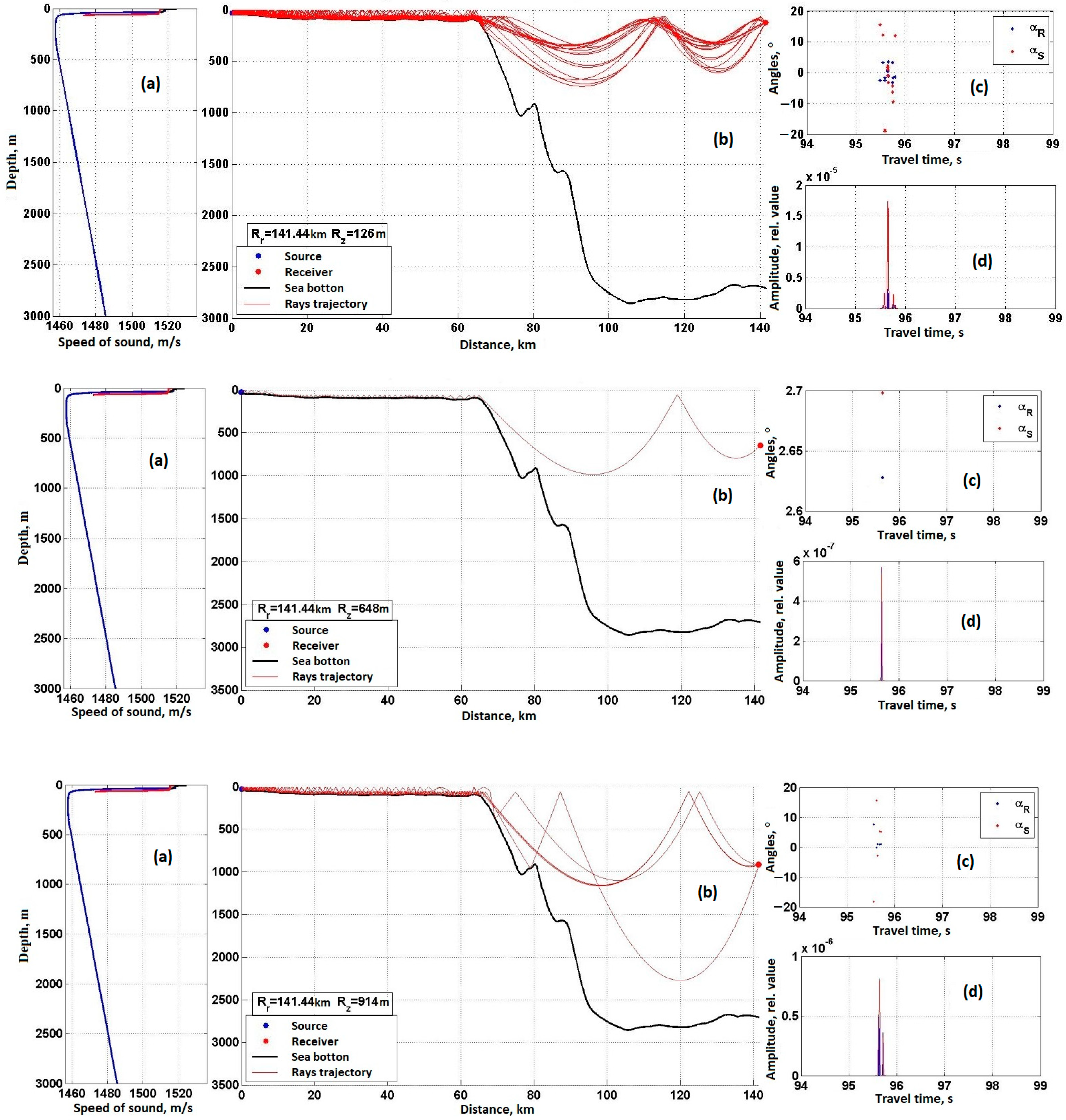
The characteristics of the waveguide’s impulse responses changed considerably with depth. Close to the USC axis, predominately a single strong pulse is detected. However, at increased depths, up to three delayed impulses can be perceived, typically with delays ranging from 20 to 30 ms, and any of these impulses may reach maximal amplitude. Since the distances between the sound source and receivers are determined based on the arrival time of the pulse with the highest magnitude, this arrival pattern can result in distance estimation inaccuracies of about 40 to 60 m.

-

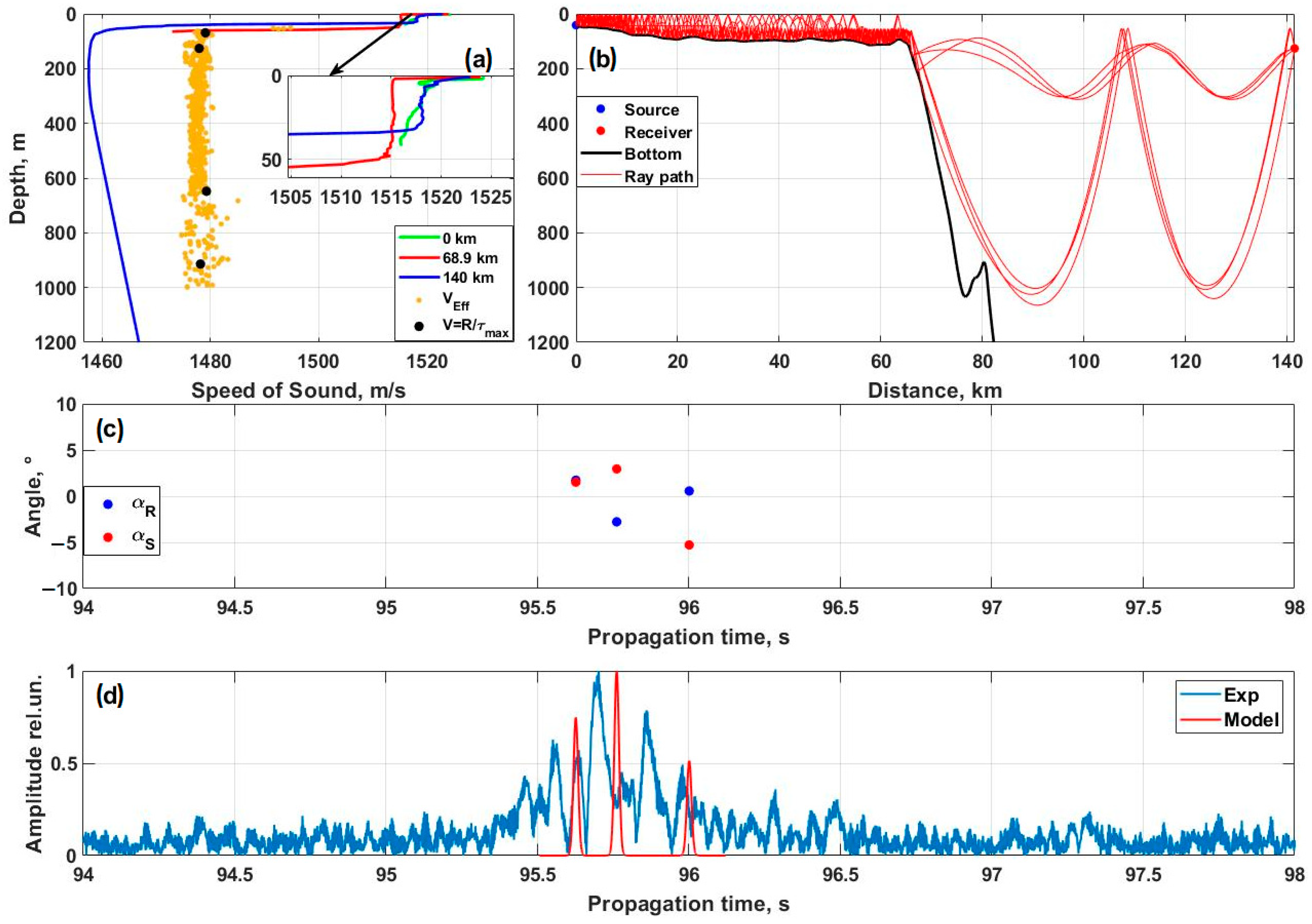
The effective velocities measured while receiving navigation signals and those computed using the proposed methodology at depths up to 500 m and distances of up to 200 km are closely aligned, differing by no more than 1 m/s from the speed of sound at the USC axis. It is noteworthy that effective velocities often necessitate correction due to the influence of the shelf area. However, in this study, such corrections were not required since the effective velocity measured in the shelf region (1456 m/s) matched the minimum group velocities.

2. Means and Methods

2.1. Deep-Sea Autonomous Measuring System

The deep-sea autonomous measuring system comprises multiple non-directional hydrophones that can be positioned at any point along a 1 km halyard. Each hydrophone is engineered for the continuous monitoring of sound pressure and current depth at the signal reception location.

Information from the hydrophone and depth sensor is organized and accumulated into data packets (frames) by an autonomous digital recording unit, which stores recordings on an SD card. After the card is removed, the data can be unpacked and converted into standard audio and text formats.

This system allows for quick deployment at designated locations within the operational area. Its compact size and lightweight design enable it to function effectively in both drifting and anchored configurations. Additionally, setup and data collection can be efficiently executed using small floating craft. The appearance of autonomous hydrophones in hermetic containers is shown in Figure 1.

Specifications:

-

Dimensions of each autonomous hydrophone—350 × Ø75 mm;

-

Number of autonomous hydrophones—4 pcs.;

-

Weight of the assembled set of autonomous hydrophones in water—13.6 kg, in air—20.64 kg;

-

Sensitivity of hydrophones—160 μV/Pa;

-

ADC bit depth—16;

-

Format of stored data—Signed Integers 16;

-

Operating frequency band—40–12,000 Hz;

-

Sampling frequency—24 kHz;

-

Intrinsic noise of amplifiers—does not exceed 63 μV/√Hz;

-

Storage device type—SDHC card up to 32 GB;

-

Power supply autonomy—12 h;

-

Battery type—Li-Ion;

-

Autonomy by data storage capacity—(32 GB-7 days, 16 GB-3 days);

-

Depth sensor—strain gauge transducer D10-T (Microtenzor Company, Orel city, Russia);

-

Depth determination accuracy—±0.1 m;

-

Depth sensor sampling frequency—4 Hz.

The setting system (Figure 2) includes an 8 mm in diameter halyard with a buoyancy (plastic buoys), a selective end with a pole, and shock-absorbing longlines.

A GPS receiver is mounted on the pole to relay location information about the system to the support vessel via a radio channel. The autonomous hydrophones are secured to the halyard with quick-release clamps. Each hydrophone’s installation depth is determined by the markings on the halyard. To adjust the depth, the entire system is raised onto the vessel, allowing the clamps to be loosened and the hydrophones repositioned along the halyard. To protect the halyard and hydrophones from vibrations caused by surface waves and currents, shock-absorbing longlines are strategically distributed by depth. The halyard is a continuous piece without knots, threaded through the block of the vessel’s lifting boom during both installation and retrieval of the system.

The electronic part of the device, located in hermetic containers, includes (Figure 3) a hydrophone signal amplification circuit with an analog low- and high-pass filter, a 16-bit analog-to-digital converter (ADC), an STM32F103 microcontroller, a depth detection module, an SD card-based data storage device, and a power supply unit (PSU) that supports autonomous operation of the device for 12 h. The PSU is divided into two blocks, for powering the digital and analog parts of the device. It is divided to reduce interference in the recording circuit from the digital part of the device.

In the block diagram:

-

ADC—16-bit analog-to-digital converter: acoustic channels—ADS8332, depth channel—ADS1110,

-

PSU—power supply unit (Li-Ion batteries of size 18,650),

-

STM32—STM32F103RC microcontroller,

-

Depth sensor—D10-T strain gauge transducer,

-

TCXO—8 MHz temperature-compensated generator.

2.2. High Power Low Frequency Acoustic Source

One of the most successful concepts for creating a high-power, low-frequency acoustic source is a technical solution based on a piston-type emitter [24,25,26], which implements the advantages potentially provided by this type of emitter, namely:

-

Using a transducer without compensating for external hydrostatic pressure, since the maximum operating depth of the emitter is determined by the yield strength of the materials used and the mechanical stresses that arise in the structure when exposed to hydrostatic pressure;

-

The possibility of significantly increasing the effective area of the radiating surface relative to the cross-sectional area of the active element, using the developed surface of the emitter body;

-

Combining the functions of the radiating aperture and the supporting structure for the elastic elements performing the preliminary stress of the active piezoceramic element by the emitter body.

The emitter contains two conical radiating surfaces connected to each other by a flexible elastic junction in the form of a ring-spring, which together form a sealed shell. Between the tops of the radiating surfaces there is an active element—a column of parallel-connected piezoceramic washers with alternating polarization, made of piezoceramic material and electrically isolated from the housing by insulating washers. When an alternating electric voltage is applied, the active element performs reciprocating longitudinal oscillations transmitted through the end elements to the radiating surfaces. The electrical impedance of such a converter is determined by the interaction of the mechanical and electrical subsystems, as well as the influence of the added mass of water. The design of such an acoustic source allows its use without compensation for hydrostatic pressure to depths of 300 m and more; it has an efficiency of up to 80%, and acoustic pressure of up to 20 kPa × m for tonal, chirping, and phase-shift keyed signals. The outer view of such source is shown in Figure 4.

Specification:

Diameter—1400 mm;

Height—1450 mm;

Mass—600 kg;

Maximum effective value of voltage—1500 V;

Efficiency on resonance frequency—more than 70%;

Estimated useful life—10¹¹ cycles;

Maximum operating depth without compensator—200 m.

Operating frequency band—300–600 Hz

2.3. Experiment Conditions

Figure 5 shows the VDSS, which demonstrates the difference between the hydrological situation on the shelf in 2023 after the passage of the typhoon and the usual situation for the summer–autumn season in 2018. The research was designed to measure the impulse characteristics of a waveguide, including the shelf and deep sea, when receiving low-frequency, phase-shift keyed signals at depths of up to 1000 m and at a distance of about 144 km from the signal source. Impulse responses were used to calculate effective sound propagation velocities when receiving signals at various depths.

The experimental protocol proceeded as follows: A broadband acoustic source was suspended from the side of an anchored vessel, positioned 150 m from the shoreline at a depth of 25 to 30 m (with a total place depth of 40 m). This source was connected to the onboard control station via a cable. Every 6 min, a complex phase-manipulated signal (M-sequence, comprising 1023 symbols and 16 carrier frequency periods per symbol) was transmitted, centered around a frequency of 400 Hz and bandwidth 375–425 Hz. The radiation session lasted for over 12 h. The layout of the experimental setup is illustrated in Figure 6.

A distributed vertical receiving system was employed to gather signal information, consisting of multiple autonomous non-directional hydrophones strategically placed at various points along a halyard that exceeded 1000 m in length and linked to a drifting rod. A GPS receiver was attached to the pole, transmitting the system’s location data to the support vessel through a radio channel. Each hydrophone was specifically designed to continuously monitor sound pressure and the current depth at the point of signal reception.

During the installation process from the yacht, “Svetlana”, autonomous hydrophones were secured to the halyard with quick-release clamps at predetermined locations along the route. The mounting depths of each hydrophone were established following hydrological measurements that addressed the objectives of the experiment. In this instance, the depths recorded were 69, 126 m (the USC axis depth), 648, and 914 m. At these depths, radiation sessions were conducted, and the received signals were convolved with a mask of the emitted signal to determine the impulse response of the waveguide at the specified depths.

3. Results

Figure 7 shows results of impulse response calculation taken from different depths.

An examination of how the structure of impulse characteristics varies with depth, as depicted in Figure 7, shows that the receiving system can detect signals starting at a depth of 69 m, with maximum amplitude occurring at 126 m, which aligns with the deepening of the USC axis. Across all measured depths, the signal’s energy is predominantly encapsulated in a burst of pulses that lasts 0.5 s, featuring the strongest pulse located near the center. The surprisingly analogous impulse characteristics detected at both the USC axis and different depths can be linked to the distinctive properties of the vertical distributed receiving system (VDSS) on an extended shelf, particularly due to substantial water mixing following the typhoon (see Figure 5).

The lack of a clear near-bottom sound propagation channel—contrasting with findings from the 2018 VDSS—resulted in enhanced illumination of the near-axial depths of the USC. Nonetheless, the highest amplitude of incoming acoustic energy was measured at 126 m, supporting the notion that its propagation follows a path closely resembling a straight line. To meet the objectives of this study, calculations were performed to evaluate the effective speed of pulse signal transmission from the source to the receivers at different depths. Effective velocities were calculated by dividing the distance between the acoustic emitter and receiver, as obtained from GPS data, by the travel time derived from the moment the maximum peak of the impulse response was detected.

The results of the calculations revealed a significant finding: the propagation times and effective velocities (approximately 1478 m/s) are nearly identical at the depth of the USC axis and at depths extending up to 914 m. This phenomenon can be understood through the lens of ray theory in sound propagation. The highest concentration of acoustic energy near the USC axis arises from signals traveling at angles close to zero, with their speeds showing minimal deviation from the sound speed at that axis. By contrast, pulse arrivals detected at considerable depths (well beneath the USC axis) correspond to sound waves moving at larger angles relative to the channel axis. These pulses navigate longer ray paths, featuring turning points at greater depths where the sound speed significantly exceeds that at the USC axis.

In this context, the interplay between the increased length of the trajectory and the heightened sound speed balances one another, leading to nearly uniform propagation times and effective speeds across all measured depths. This concept can be visually illustrated through diagrams produced using the RAY [27,28] program, which operates within the framework of ray theory in sound propagation (see Figure 8).

For a more detailed analysis and physical interpretation of the obtained experimental data, numerical modeling of the dependence of sound speed on depth was carried out using the RAY program. To carry out the calculations, the above data on the hydrological and bathymetric parameters of the waveguide were used. The average bottom inclination angle on the shelf is β = 0.06 degrees. Depth at the point of radiation z₀ = 42 m, depth of the emitter z_S = 35 m. Deep-sea average depth is about 3 km. The distance between the emitter and the receiver is R = 141.44 km. As a result of numerical modeling, the eigenrays between the acoustic source and the receiver and the impulse characteristics of the waveguide were calculated at a depth range from 60 to 1000 m with a step between horizons of 1 m. Next, the propagation time τ_MAX was calculated, corresponding to the maximum arrival of the impulse response (IR) energy. In most IRs, the maximum was located in the middle. At the last stage, to calculate the effective speed of sound, the distance between the source and receiver was divided by the propagation time: V_EFF = R/τ_MAX.

4. Discussion

Upon examining Figure 9, it is evident that the calculated model using effective speeds of sound (depicted by orange dots) for each horizon closely align with the effective speeds of sound (represented by black dots) observed during the experiment. The accuracy stands at about 1 m/s for a horizon of 600 m and 0.1 m/s for other horizons. While the objective of achieving an exact match between the calculated and experimentally obtained impulse responses (IRs) was not established, numerical confirmation was obtained regarding the expansion of the waveguide pulse response to 0.5 s and the presence of a maximum arrival in the middle, mirroring the experimental findings. This suggests the potential utility of the RAY program for modeling and interpreting the physical processes of acoustic wave propagation in intricate hydrological and bathymetric conditions.

In earlier works by the authors [29,30], it was experimentally demonstrated that errors in distance measurements using acoustic methods, when employed to calculate signal propagation times and sound speeds on the USC axis, do not exceed 100–150 m when the USC is up to 200 miles offshore. Consequently, the aforementioned results regarding the equality of effective velocities when receiving on the USC axis and at other depths allow us to anticipate similar positioning accuracy when conducting actual maneuvers of the DSAMS group at depths of up to 1000 m and distances spanning hundreds of kilometers from control posts.

This study reveals a significant detail: unlike the experimental data from the Philippine Sea, our findings indicate that the effective (i.e., group) signal propagation velocity shows minimal variation with depth. In other words, the bathymetry and hydrological conditions of the studied region play a crucial role in shaping the distribution of group velocities with depth. Specifically, two separate studies in the Sea of Japan have confirmed that the group velocity remains largely constant within the depth range of 200 to 1000 m.

5. Conclusions

In conclusion, we summarize the key findings and insights drawn from achieving the objectives of this study.

• The results obtained are of both fundamental and practical significance for tackling the challenges of positioning and control associated with DSAMS during missions that occur at considerable distances of hundreds of kilometers from SNS and at depths reaching up to 1000 m. The experiment detailed in this article represents a technical and methodological extension of the study outlined in Section 1.2, yet it was conducted under markedly different climatic conditions resulting from the aftermath of a strong typhoon in the surveyed region. This extension greatly improves the potential for advancing both theory and practical approaches to these challenges.
• This study highlighted practical considerations related to the formation of the impulse response in the waveguide following the impact of the powerful typhoon that affected the surveyed waters. The absence of a near-bottom sound channel on the shelf, which typically develops during summer due to water mixing, resulted in the impulse characteristics of the waveguide at all depths manifesting as a series of pulses lasting 0.5 s, with the peak amplitude pulse situated nearer to the center. Additionally, it was observed that the times and effective propagation speeds of maximum pulses remained roughly constant across all depths, illustrating their practical utility in addressing positioning issues for underwater robotic units operating at depths up to 1000 m.
• Numerical modeling conducted with the RAY program, based on ray approximation, demonstrated that the calculated effective velocities for each horizon closely matched the experimentally observed effective velocities, achieving an accuracy of about 1 m/s for a depth of 600 m and 0.1 m/s for other depths. Importantly, numerical evidence confirmed the expansion of the waveguide impulse response to 0.5 s and identified the presence of a peak arrival in the center, which was also observed in the experiments. This finding indicates the potential for using the RAY program to model and analyze the physical processes of acoustic wave propagation in complex hydrological and bathymetric environments.
• The distinctive and practically valuable experimental and theoretical outcomes derived from acoustic range-finding measurements conducted over various years—simulating real maneuvering scenarios of multiple underwater robots at depths of up to 1000 m and hundreds of kilometers from control stations—underscore the need for further extensive research. Such investigations should leverage advanced technologies and theoretical modeling methods.

References

1. Li, P.; Wang, D.; Wang, L.; Lu, H. Deep visual tracking: Review and experimental comparison. Pattern Recognit. 2018, 76, 323–338. [Google Scholar] [CrossRef]
2. Badiey, M.; Katsnelson, B.G.; Lynch, J.F.; Pereselkov, S.; Siegmann, W.L. Measurement and modeling of three-dimensional sound intensity variations due to shallow-water internal waves. J. Acoust. Soc. Am. 2005, 117, 613–625. [Google Scholar] [CrossRef] [PubMed]
3. ATOC Consortium. Ocean climate change: Comparison of acoustic tomography, satellite altimetry, and modeling. Science 1998, 281, 1327–1332. [Google Scholar] [CrossRef] [PubMed]
4. Camus, L. Autonomous Surface and Underwater Vehicles as Effective Ecosystem Monitoring and Research Platforms in the Arctic–The Glider Project. Sensors 2021, 21, 6752. [Google Scholar] [CrossRef]
5. Wolfson, M.A.; Spiesberger, J.L.; Tappert, F.D. Internal wave effects on long-range ocean acoustic tomography. J. Acoust. Soc. Am. 1995, 97, 3235. [Google Scholar] [CrossRef]
6. Martin, B. An Analysis of Current and Future Technology for Unmanned Maritime Vehicles; RAND Corporation: Santa Monica, CA, USA, 2019. [Google Scholar]
7. Worcester, P.F.; Cornuelle, B.D.; Dzieciuch, M.A.; Munk, W.H.; Howe, B.M.; Mercer, J.A.; Spindel, R.C.; Metzger, K.; Birdsall, T.G. A test of basin-scale acoustic thermometry using a large-aperture vertical array at 3250-km range in the eastern North Pacific Ocean. J. Acoust. Soc. Am. 1999, 105, 3185–3201. [Google Scholar] [CrossRef]
8. Baggeroer, A.B.; Sperry, B.; Lashkari, K.; Chiu, C.-S.; Miller, J.H.; Mikhalevsky, P.N.; von der Heydt, K. Vertical array receptions of the Heard Island transmissions. J. Acoust. Soc. Am. 1994, 96, 2395–2413. [Google Scholar] [CrossRef]
9. Cornuelle, B.D.; Worcester, P.F.; Hildebrand, J.A.; Hodgkiss, W.S., Jr.; Duda, T.F.; Boyd, J.; Howe, B.M.; Mercer, J.A.; Spindel, R.C. Ocean acoustic tomography at 1000-km range using wave fronts measured with a large-aperture vertical array. J. Geophys. Res. 1993, 98, 16365–16377. [Google Scholar] [CrossRef]
10. Galkin, O.P.; Pankova, S.D. Correlation characteristics and travel time differences for hydroacoustic signals under directional reception at different depths. Acust. Zhurnal 2003, 49, 481–488. [Google Scholar] [CrossRef]
11. Vadov, R.A. Long-range sound propagation in the norwegian sea. Acoust. Phys. 2002, 48, 24–33. [Google Scholar] [CrossRef]
12. Vadov, R.A. Long-range sound propagation in the central region of the Baltic Sea. Acoust. Phys. 2001, 47, 150–159. [Google Scholar] [CrossRef]
13. Vadov, R.A. Long-range sound propagation in the northwestern region of the Pacific Ocean. Acoust. Phys. 2006, 52, 377–391. [Google Scholar] [CrossRef]
14. Vadov, R.A. Long-range sound propagation in the northeastern Atlantic. Acoust. Phys. 2005, 51, 629–637. [Google Scholar] [CrossRef]
15. Vadov, R.A. Long-range sound propagation in the shallow-water part of the Sea of Okhotsk. Acoust. Phys. 2002, 48, 142–146. [Google Scholar] [CrossRef]
16. Vadov, R.A. Peculiarities in the formation of the sound field structure of a point source in the Black Sea underwater sound channel. Acoust. Phys. 2011, 57, 642–651. [Google Scholar] [CrossRef]
17. Vadov, R.A. Some features of the formation of sound fields in the Kamchatka region of the Pacific Ocean. Akust. Zhurnal 2002, 48, 751–759. [Google Scholar] [CrossRef]
18. Vadov, R.A. Some results of studies of long-distance sound propagation in the Greenland Sea. Akust. Zhurnal 2000, 46, 47–59. [Google Scholar]
19. Vadov, R.A. Point source field in an underwater sound channel in the Sea of Japan. Akust. Zhurnal 1998, 44, 601–609. [Google Scholar]
20. Worcester, P.F.; Dzieciuch, M.A.; Mercer, J.A.; Andrew, R.K.; Dushaw, B.D.; Baggeroer, A.B.; Heaney, K.D.; D’Spain, G.L.; Colosi, J.A.; Stephen, R.A.; et al. The North Pacific Acoustic Laboratory deep-water acoustic propagation experiments in the Philippine Sea. J. Acoust. Soc. Am. 2013, 134, 3359–3375. [Google Scholar] [CrossRef]
21. Graupe, C.; Van Uffelen, L.; Worcester, P.F.; Dzieciuch, M.A.; Howe, B.M. An automated framework for long-range acoustic positioning of autonomous underwater vehicles. J. Acoust. Soc. Am. 2022, 152, 1615–1627. [Google Scholar] [CrossRef]
22. Mikhalevsky, P.; Sperry, B.J.; Woolfe, K.F.; Dzieciuch, M.A.; Worcester, P.F. Deep ocean long range underwater navigation with ocean circulation model corrections. J. Acoust. Soc. Am. 2023, 154, 548–559. [Google Scholar] [CrossRef]
23. Chang, K.I.; Zhang, C.I.; Park, C.; Kang, D.J.; Ju, S.J.; Lee, S.H.; Wimbush, M. (Eds.) Oceanography of the East Sea (Japan Sea); Springer International Publishing: Cham, Switzerland, 2016; 460p. [Google Scholar]
24. Britenkov, A.K.; Farfel, V.A.; Bogolyubov, B.N. Comparison and analysis of electroacoustic characteristics of high power density compact low frequency hydroacoustic transducers. Appl. Phys. 2021, 3, 72–77. [Google Scholar] [CrossRef]
25. Rimsky-Korsakov, A.V.; Yamshchikov, V.S.; Zhulin, V.I.; Rekhtman, V.I. Akusticheskie Podvodnye Nizkochastotnye Izluchateli–L.; Sudostroenie: St. Petersburg, Russia, 1984; 184p. [Google Scholar]
26. Bogorodskij, V.V.; Zubarev, L.A.; Korepin, E.A.; Yakushev, V.I. Podvodnye Elektroakusticheskie Preobrazovateli–L.; Sudostroenie: St. Petersburg, Russia, 1983; 248p. [Google Scholar]
27. Boden, L.; Bowlin, J.B.; Spiesberger, J.L. Time domain analysis of normal mode, parabolic, and ray solutions of the wave equation. J. Acoust. Soc. Am. 1991, 90, 954–958. [Google Scholar] [CrossRef]
28. Bowlin, J.B.; Spiesberger, J.L.; Duda, T.F.; Freitag, L.E. Ocean Acoustical Ray-Tracing Software RAY; Woods Hole Oceano-Graphic Technical Report; WHOI-93-10; Woods Hole Oceanographic Institution: Woods Hole, MA, USA, 1993. [Google Scholar]
29. Morgunov, Y.N.; Bezotvetnykh, V.V.; Burenin, A.V.; Voitenko, E.A. Study of how hydrological conditions affect the propagation of pseudorandom signals from the shelf in deep water. Acoust. Phys. 2016, 62, 350–356. [Google Scholar] [CrossRef]
30. Morgunov, Y.N.; Bezotvetnykh, V.V.; Golov, A.A.; Burenin, A.V.; Lebedev, M.S.; Petrov, P.S. Experimental study of the impulse response function variability of underwater sound channel in the Sea of Japan using pseudorandom sequences and its application to long-range acoustic navigation. Acoust. Phys. 2021, 67, 287–292. [Google Scholar] [CrossRef]
Figure 1. The appearance of autonomous hydrophones in hermetic containers.
Jmse 12 02365 g001
Figure 2. A scheme of DSAMS mounting.
Jmse 12 02365 g002
Figure 3. Block-scheme of the electronic part of the DSAMS.
Jmse 12 02365 g003
Figure 4. The outer view of a high-power, low-frequency acoustic source based on a piston-type emitter.
Jmse 12 02365 g004
Figure 5. Measured vertical distribution of sound speed at the emission point in 2018 and after typhoon “Khanun” in 2023.
Jmse 12 02365 g005
Figure 6. The scheme of the conducted experiments.
Jmse 12 02365 g006
Figure 7. Pulse characteristics of the waveguide obtained at the depths of 69, 126, 680, and 914 m.
Jmse 12 02365 g007
Figure 8. Results of raytracing using the “RAY” algorithm: (a) VDSS at points along the route; (b) ray pattern of propagation of acoustic signals; (c) emission and arrival angles; (d) impulse response.
Jmse 12 02365 g008aJmse 12 02365 g008b
Figure 9. Results of numerical modeling: (a) vertical distributions of sound speed near the source and at receiving points (blue, red, and green curve); the vertical distribution of the effective speed of sound calculated in the ray approximation (orange dots); experimentally measured values of the effective speed of sound at given depths using the impulse characteristics of the waveguide (black dots); (b) bottom topography and an example of a ray pattern for an acoustic path when receiving at a depth of 126 m; (c) angular structure of the field at the receiving point (red dots are the source angles, blue dots are the receiver angles); (d) impulse response of the waveguide at the receiving point at a horizon of 126 m (the experimental IR is shown in blue, and the simulated one in red).
Jmse 12 02365 g009
Disclaimer/Publisher’s Note: The statements, opinions and data contained in all publications are solely those of the individual author(s) and contributor(s) and not of MDPI and/or the editor(s). MDPI and/or the editor(s) disclaim responsibility for any injury to people or property resulting from any ideas, methods, instructions or products referred to in the content.