Underwater SSP Measurement and Estimation: A Survey

Abstract

Real-time and accurate construction of regional sound speed profiles (SSPs) is important for building underwater positioning, navigation, and timing (PNT) systems as it greatly affects signal propagation modes. In this paper, we summarize and analyze the current research status in the field of underwater SSP construction, where the mainstream methods include direct SSP measurement and SSP inversion. For the direct measurement method, we compare the performance of popular international and commercial brands of temperature, conductivity, and depth profilers (CTDs). For the inversion methods, the framework and basic principles of matched field processing (MFP), compressive sensing (CS), and deep learning (DL) are introduced, and their advantages and disadvantages are compared. Presently, SSP inversion relies on sonar observation data, limiting its applicability to areas that can only be reached by underwater observation systems. Furthermore, these methods are unable to predict the distribution of sound velocity in future time. Therefore, the mainstream trend in future research on SSP construction will involve comprehensive utilization of multi-source data to offer elastic sound velocity distribution estimation services for underwater users without the need for sonar observation data.

1. Introduction

The construction of underwater integrated positioning, navigation, timing, and communication (PNTC) systems is of great significance for early warning of marine disasters, underwater rescues, exploration of marine resources, and national security [1]. With the development of sensing technology and underwater robotics, establishing multi-source, real-time, and three-dimensional observation networks becomes an important way for achieving underwater PNTC systems. These networks consist of devices such as surface buoys, dive beacons, bottom anchors, autonomous underwater vehicles (AUVs), and underwater remotely operated vehicles (ROVs).

Positioning and communication are the two most important technical foundations of underwater PNTC service systems. Not only do the underwater frogman, submarine, and other user’s equipment need accurate PNTC services, but the ocean temperature, salinity information collection, and biological activity information perception also need to be accompanied by accurate positioning information. At the same time, the perceived and collected information needs to be transmitted back to the ground information processing center in time to be utilized, so how to improve the efficiency and accuracy performance of underwater communication and positioning has been widely focused on by scholars for a long time.

In the underwater environment, the attenuation of acoustic signals is much smaller than that of radio signals and optical signals, thus the acoustic signal becomes the main signal carrier of the underwater PNTC system. However, because of the influence of non-uniformly distributed underwater temperature, salinity, and pressure, the propagation speed of acoustic signals has complex dynamic spatial and temporal changing characteristics, which leads to the bending of the signal propagation path due to the Snell effect. The signal bending phenomenon poses great challenges for the efficient utilization of beam energy in directional communication systems and high-precision ranging in acoustic localization [2]. If the regional sound speed distribution could be obtained, the signal propagation trajectory can be tracked and reconstructed according to the ray-tracing theory [3,4,5], which promotes the development of high precision of positioning, ranging, and timing as well as high efficiency of communication in the PNTC service system. Therefore, real-time and accurate sound speed field construction is of significant importance.

To give a comprehensive understanding of the development of underwater sound speed field construction, we investigate and compare methods for sound speed field construction. The contribution of our work is summarized as follows:

• We have conducted a survey on sound speed field construction indicating that it can be obtained by two kinds of methods: direct measurement method and inversion method.
• We have summarized the recognized mainstream underwater sound speed empirical formulas and compared their application scenarios.
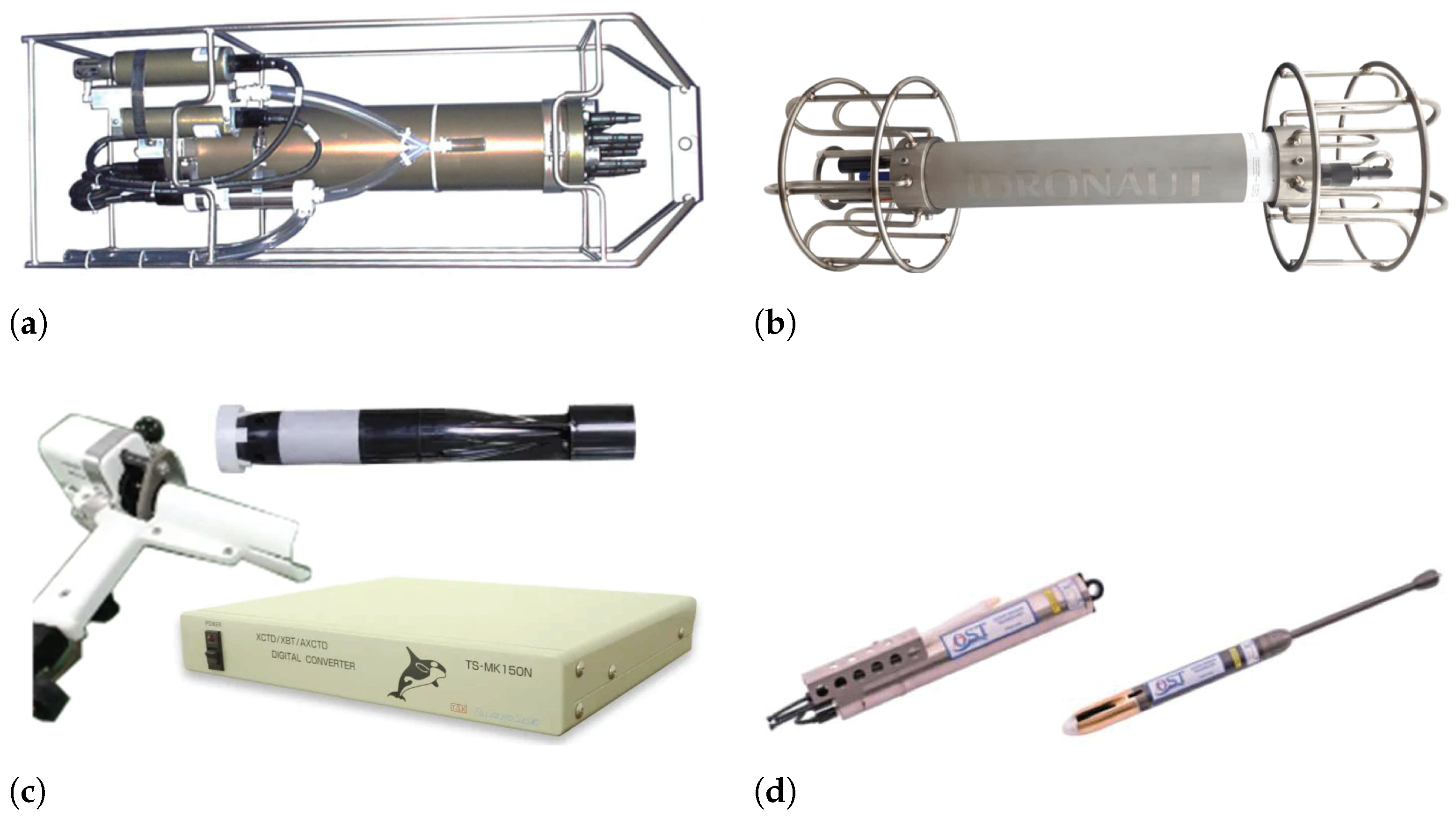
• We have conducted research on advanced global commercial temperature, conductivity, and depth profiler (CTD), and compared their performance indicators.
• We have summarized three frameworks for constructing sound speed fields: matched field processing (MFP), compressive sensing (CS), and deep learning (DL). We have also compared the performance of different sound field construction methods.
• We have reviewed the development of constructing sound speed fields, identified current problems to be solved, and identified the trends of future development.

The organization of this paper is elaborated below. Section 2 provides a classification of methods for constructing sound speed fields, summarizes empirical formulas for sound speed, and compares the advanced commercial equipment used in direct measurement methods around the world. Section 3 summarizes three mainstream frameworks for sound speed field inversion and provides a detailed introduction to different methods. A comparison of methods for constructing underwater sound speed fields is given in Section 4, and conclusions are drawn in Section 5.

2. Methods for Constructing Underwater Acoustic Velocity Fields

Underwater sound speed distribution has dynamic spatial and temporal differences. For a similar scale of distance, the change of sound speed in the vertical direction is much larger than that of the horizontal direction, so sound speed profiles (SSPs) are usually adopted to describe the distribution of the sound speed field in a small-scale region. Currently, the mainstream methods for obtaining the underwater SSP include direct measurement and SSP inversion.

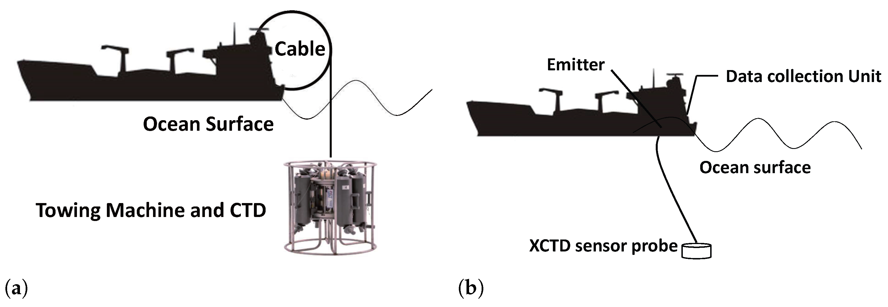
2.1. Direct Measurement Methods

The attempt to measure sound velocity can be traced back to the Lake Geneva experiment in 1827. Colladon and Sturm collaborated to use sound tubes for receiving the ringing sound of a distant diving bell [6]. The Lake Geneva experiment measured the speed of sound propagation for the first time in lake water, but it was not possible to obtain the variation of sound speed with depth because of the limited experimental conditions.

With the development of electronic instruments, sound velocity profilers (SVPs) appeared in the 1950s, which utilized the acoustic pulse signal for direct measurement of sound speed. Typical SVPs include the sound speed change recorder developed by Brown based on the phase method in 1953, the “ring-tone” SVP developed by Greenspan and Tschiegg based on the pulse method in 1957, and the low-frequency SVP developed by Scheffel based on the resonance method in 1960 [7]. SVP can measure the absolute value of sound speed, but the equipment is not easy to miniaturize. Moreover, SVP is not conducive to exploring the spatial–temporal changes in global sound speed distribution, so it is difficult to carry out the sound speed forecasting.

In 1960, Wilson et al. summarized an accurate empirical formula of sound speed distribution [8,9], which promoted the rapid development of underwater sensing equipment. From then on, underwater SVPs can be measured using instruments such as the CTD or the more portable and smaller expendable CTD (XCTD) that works together with empirical sound speed formulas [10]. In addition, Leroy, Grosso, Medwin, etc. have each proposed empirical formulas under different applicable conditions, and the most commonly used empirical formulas for calculating sound speed and their scope of application are listed as follows:

(1)

Wilson empirical formula [8]:

$$\begin{array}{cc}\hfill v& =1449.14+v_t+v_p+v_s+v_{tpS}\hfill \\ \hfill v_t& =4.5721t-4.4532\times {10}^{-2}{t}^2-2.604\times {10}^{-4}{t}^3\hfill \\ \hfill & +7.9851\times {10}^{-6}{t}^4\hfill \\ \hfill v_p& =1.60272\times {10}^{-1}p+1.0268\times {10}^{-5}{p}^2\hfill \\ \hfill & +3.5216\times {10}^{-9}{p}^3-3.3603\times {10}^{-12}{p}^4\hfill \\ \hfill v_s& =1.39799(S-35)+1.69202\times {10}_{-3}{(S-35)}^2\hfill \\ \hfill v_{tpS}& =(S-35)(-1.1244\times {10}^{-2}t+7.7711\times {10}^{-7}{t}^2\hfill \\ \hfill & +7.7016\times {10}^{-5}p-1.2943\times {10}^{-7}{p}^2\hfill \\ \hfill & +3.1580\times {10}^{-8}pt+1.5790\times {10}^{-9}p{t}^2)\hfill \\ \hfill & +p(-1.8607\times {10}^{-4}t+7.4812\times {10}^{-6}{t}^2\hfill \\ \hfill & +4.5283\times {10}^{-8}{t}^3)+p^2(-2.5294\times {10}^{-7}t\hfill \\ \hfill & +1.8563\times {10}^{-9}{t}^2)+p^3(-1.9646\times {10}^{-10}t)\hfill \end{array}$$

(1)

where t is the temperature in °C, S is the salinity in ‰, and p is the pressure in kg/cm³. The W.D. Wilson formula can be applied over the range of temperature [−4 °C, 30 °C], salinity $[0, 37]$, and pressure [$0,1000$ kg/cm³].

(2)

Leroy empirical formula [11]:

$$\begin{array}{cc}\hfill v& =1.492.9+3(t-10)-0.006{(t-10)}^2-0.04{(t-18)}^2\hfill \\ \hfill & +1.2(S-10)-0.01(S-35)(T-18)+Z/61\hfill \end{array}$$

(2)

where t is the temperature in °C, S is the salinity in ‰, and Z is the depth in m. Leroy’s empirical formula can be applied over the range of temperature $[-2 °\mathrm{C}$, $34 °\mathrm{C}$], salinity $[20, 42]$, and depth up to 8000 m.

(3)

Medwin empirical formula [12]: In 1975, Medwin proposed a simplified formula based on the Wilson empirical formula:

$$\begin{array}{cc}\hfill v& =1449.2+4.6t-0.055t^2+0.00029t^3\hfill \\ \hfill & +(1.34-0.01t)(S-35)+0.016Z\hfill \end{array}$$

(3)

where $t,S$, and Z have the same meaning and unit with Leroy’s empirical formula. The Medwin empirical formula can be applied over the range of temperature $[0, 35 °\mathrm{C}$], salinity $[0, 45]$, and depth up to 1000 m.

(4)

Del Grosso empirical formula [13]: In 1974, Del Grosso summarized the empirical formula for calculating sound speed under conditions with high salinity:

$$\begin{array}{cc}\hfill v& =1402.392+\Delta v_t+\Delta v_s+\Delta v_p+\Delta v_{tpS}\hfill \\ \hfill \Delta v_t& =0.501109398873\times 10t-0.550946843172\times {10}^{-1}{t}^2\hfill \\ \hfill & +0.221535969240\times {10}^{-3}{t}^3\hfill \\ \hfill \Delta v_s& =0.132952290781\times 10S\hfill \\ \hfill & +0.128955756844\times {10}^{-3}{S}^2\hfill \\ \hfill \Delta v_p& =0.156059257041\times p+0.244998688441\times {10}^{-4}{p}^2\hfill \\ \hfill & -0.883392332513\times {10}^{-8}{p}^3\hfill \\ \hfill \Delta v_{tpS}& =-0.127562783426\times {10}^{-1}tS\hfill \\ \hfill & +0.635191613389\times {10}^{-2}tp\hfill \\ \hfill & +0.265484716608\times {10}^{-7}{t}^2{p}^2\hfill \\ \hfill & -0.159349479045\times {10}^{-5}t{p}^2\hfill \\ \hfill & +0.522116437235\times {10}^{-9}t{p}^3\hfill \\ \hfill & -0.438031096213\times {10}^{-6}{t}^{3}p\hfill \\ \hfill & -0.161674495909\times {10}^{-8}{S}^2{p}^2\hfill \\ \hfill & +0.968403156410\times {10}^{-4}{t}^{2}S\hfill \\ \hfill & +0.485639620015\times {10}^{-5}t{S}^{2}p\hfill \\ \hfill & -0.340597039004\times {10}^{-3}tpS\hfill \end{array}$$

(4)

where $t,S$, and p have the same meaning and unit with the Wilson empirical formula. Del Grosso’s empirical formula is applicable to the following ranges: temperature $[0, 30 °\mathrm{C}$], salinity $[30, 40]$, and pressure $[0, 1000$ kg/cm³].

(5)

Chen–Millero empirical formula [14]: In 1977, Chen and Millero, transmitting Wilson’s data to more accurately measured sound speed data, proposed the Chen–Millero empirical formula by studying Wilson’s measurements data:

$$\begin{array}{cc}\hfill v& =C_w(t,p)+A(t,p)S+B(t,p)S^{3/2}+D(t,p)S^2\hfill \\ \hfill C_w(t,p)& =(C_{00}+C_{01}t+C_{02}{t}^2+C_{03}{t}^3+C_{04}{t}^4+C_{05}{t}^5)\hfill \\ \hfill & +(C_{10}+C_{11}t+C_{12}{t}^2+C_{13}{t}^3+C_{14}{t}^4)p\hfill \\ \hfill & +(C_{20}+C_{21}t+C_{22}{t}^2+C_{23}{t}^3+C_{24}{t}^4)p^2\hfill \\ \hfill & +(C_{30}+C_{31}t+C_{32}{t}^2)p^3\hfill \\ \hfill A(t,p)& =(A_{00}+A_{01}t+A_{02}{t}^2+A_{03}{t}^3+A_{04}{t}^4)\hfill \\ \hfill & +(A_{10}+A_{11}t+A_{12}{t}^2+A_{13}{t}^3+A_{14}{t}^4)p\hfill \\ \hfill & +(A_{20}+A_{21}t+A_{22}{t}^2+A_{23}{t}^3)p^2\hfill \\ \hfill & +(A_{30}+A_{31}t+A_{32}{t}^2)p^3\hfill \\ \hfill B(t,p)& =B_{00}+B_{01}t+(B_{10}+B_{11}t)p\hfill \\ \hfill D(t,p)& =D_{00}+D_{10}p\hfill \end{array}$$

(5)

where t and S have the same meaning and unit with the Medwin empirical formula, p is the pressure in bar. $C_w(t,p)$ represents the sound speed value in a purified water environment. The parameters $A(t,p),B(t,p),C_w(t,p),$ and $D(t,p)$ can be obtained by checking the table in the literature [15]. The Chen–Millero empirical formula can be applied with the following ranges: temperature $[0, 40 °\mathrm{C}$], salinity $[5, 40]$, and pressure up to 1000 bar. In 1994, Millero and Li made a more accurate correction within the low-temperature range based on the Chen–Millero empirical formula and proposed the Chen–Millero–Li formula [16], which has been recommended by the United Nations Educational, Scientific and Cultural Organization (UNESCO) as the international standard formula for calculating underwater sound speed.

(6)

Coppens empirical formula [17]: In 1981, Coppens extrapolated the Del Grosso’s formula in the ranges of high salt, low salt, and low temperature, and then proposed the Coppens empirical formula:

$$\begin{array}{cc}\hfill v& =v_0+(16.23+0.0253t)0.001Z\hfill \\ \hfill & +(0.213-0.01t)0.000001Z^2\hfill \\ \hfill & +[0.016+0.0002(S-35.0\left)\right]\times (S-35.0)0.00001tZ\hfill \\ \hfill v_0& =1449.05+4.57t-0.0521t^2+0.00023t^3\hfill \\ \hfill & +(1.333-0.0126t+0.00009t^2)\times (S-35.0)\hfill \end{array}$$

(6)

where t is the temperature in °C, S is the salinity in ‰, and Z is the depth in m. Coppens empirical formula can be applied within the ranges of temperature $[0, 35 °\mathrm{C}$], salinity $[0, 45]$, and depth up to 4000 m. The application condition of mainstream sound speed empirical formula is given in

Table 1. Comparison of different sound speed empirical formulas.

Empirical Formula	Proposed Year	Application Range
		Temperature	Salinity	Depth/Pressure
Wilson empirical formula [8]	1960	[−4 °C, 30 °C]	$[0, 37]$	[0, 1000 kg/cm3]
Leroy empirical formula [11]	1969	[−2 °C, 34 °C]	$[20, 42]$	[0, 8000 m]
Del Grosso empirical formula [13]	1974	[0, 30 °C]	$[30, 40]$	[0, 1000 kg/cm3]
Medwin empirical formula [12]	1975	[0, 35 °C]	[0, 45‰]	[0, 1000 m]
Chen–Millero empirical formula [14]	1977	[0, 40 °C]	$[5, 40]$	[0, 1000 bar]
Coppens empirical formula [17]	1981	[0, 35 °C]	$[0, 45]$	[0, 4000 m]

.

Among the direct measurement methods of sound speed, SVP can measure the absolute value of sound speed, so it is usually used as the standard of regional sound speed distribution. However, the sound speed measurement based on CTD and XCTD is more flexible and portable, but the accuracy is not as good as SVP, and different empirical formulas have different applicable ranges.

Based on multi-beam bathymetry systems, Zhou et al. studied the applicable range of mainstream sound speed empirical formulas from the perspective of determining the optimal sound speed formula [18]. Leveraging SVP measurement data from the South China Sea, Chen et al. compared and analyzed the applicable range of mainstream sound speed empirical formulas based on CTD sea trial data [19]. According to Chen’s research conclusion, the Chen–Millero–Li formula is the most suitable one for use in rivers, lakes, estuaries, coasts, and continental shelf waters. Del Grosso’s empirical formula and Coppens empirical formula are superior in the deep sea. The Wilson empirical formula is widely mentioned in educational books because it is the earliest proposed and has better stability, but its extrapolation applicability is insufficient in the area within the low-salt range.

Benefiting from the advantages of simple operation, flexibility, convenience, and easy integration of miniaturized sensors, CTD has developed rapidly since the 1950s. Developed countries such as the United States, Italy, Canada, Germany, and Japan started early in the development of CTD equipment, and after decades of development, their technology has long been leading the world. Well-known commercial CTD products mainly include the Sea Bird (SBE) series CTD produced by Sea Bird company from the U.S. [20], the SonTek CastAway CTD produced by YSI from the U.S. [21], the Ocean Seven (OS) 300 series CTD produced by Idronaut company from Italy [22], the RBR series CTD produced by RBR company from Canada [23], and the CTD detectors produced by Sea & Sun Technology from Germany [24]. While Japan pays more attention to the development of small portable products such as XCTD products produced by Tsurumi-Seiki (TSK) [25].

The development of CTD equipment in China began relatively late. However, after years of development, many types of fully independent technical products have appeared based on shipboard, fixed platforms, or underwater mobile platforms. The National Ocean Technology Center is the earliest institution to carry out CTD technology research in China and gradually formed Ocean Sensor Technology (OST) series products from 2020, which reached the international level in temperature and salinity measurements [26]. Although China’s temperature and salinity depth measurement technology has made great breakthroughs, there is still a certain gap in the depth coverage range compared to the top commercial CTDs due to the shortcoming of pressure resistance technology. Parts of commercial CTDs are given in Figure 1. The performance comparison of typical commercial CTD/XCTD is shown in

Table 2. Comparison of commercial CTD and XCTD.

Model		OST15D [26]	SBE911plus [20]	OS320plus [22]	CTD90M [24]	RBR Concerto3 [23]	XCTD-4N [25]
Temperature (°C)	Range	[−5, 35]	[−5, 35]	[−5, 45]	[−2, 36]	[−5, 35]	[−2, 35]
	Accuracy	$\pm 0.002$	$\pm 0.001$	$\pm 0.001$	$\pm 0.002$	$\pm 0.002$	$\pm 0.02$
	Resolution	0.0001	0.0002	0.0001	0.0005	<0.00005	0.01
	Stability	$\pm 0.002$/year	$\pm 0.0002$/month	-	-	$\pm 0.002$/year	-
Conductivity (S/m)	Range	[0, 7]	[0, 7]	[0, 7]	[0, 30]	[0, 8.5]	[0, 6]
	Accuracy	$\pm 0.0003$	$\pm 0.0003$	$\pm 0.0001$	$\pm 0.001$	$\pm 0.0003$	$\pm 0.003$
	Resolution	0.00001	0.00004	0.00001	0.0005	<0.0001	0.0015
	Stability	$\pm 0.0003$/month	$\pm 0.0003$/month	-	-	$\pm 0.001$/year	-
Pressure (${10}^4$ kPa)	Range	[0, 7]	[0, 10.5]	[0, 10]	[0, 6]	[0, 6]	[0, 1.85]
	Accuracy	$\pm 0.05\%$ range	$\pm 0.015\%$ range	$\pm 0.01\%$ range	$\pm 0.05\%$ range	$\pm 0.05\%$ range	-
	Resolution	$\pm 0.001\%$ range	$\pm 0.001\%$ range	$\pm 0.002\%$ range	$\pm 0.002\%$ range	$\pm 0.001\%$ range	-
	Stability	$\pm 0.05$ range/year	$\pm 0.02$ range/year	-	-	$\pm 0.05$ range/year	-
Department		Oceans Center	Sea Bird	Idronaut	SST	RBR	TSK
Country		China	the U.S.	Italy	Germany	Canada	Japan

.

The advantage of utilizing CTD (or SVP) for SSP measurement lies in good accuracy performance and high depth resolution. However, since the measurement needs to be executed by stopping the ship with the help of the ship-borne towing machine as shown in Figure 2a. Thus, the measurement period is quite long, which seriously affects the operational efficiency. For example, when the down and up speed of the cable is 50 m/min, it takes 80 min to measure the SSP at a depth of 2000 m. In contrast, XCTD measurement can be executed while the ship platform keeps sailing (within five knots). The probe falls by gravity, the data are transmitted back through the copper wire, and the probe is discarded at the end without recycling, so it does not affect the operational efficiency. For example, it only takes about 20 min to measure the SSP at a depth of 2000 m. Meanwhile, the portability of XCTD allows it to be carried on automated platforms such as drones or unmanned underwater vehicles (UUVs) [10,27,28]. However, the coverage of XCTD usually can not exceed 2000 m because of the limitation of the sensor’s pressure resistance performance. Figure 2b shows a schematic diagram of the SSP measurement using XCTD.

In order to reconstruct the full ocean depth SSP using partial ocean depth sound speed data measured by XCTD, Cheng et al. proposed an SSP extension method for land-marginal deep-water areas based on the orthogonal empirical function (EOF) decomposition [29]. Cheng effectively realized the low-precision loss extension of the SSPs. However, it requires the prior data information coverage to exceed the depth of the sound channel axis, so the application is limited. Inspired by the above method, Huang et al. also proposed an SSP extension method based on EOF decomposition [30], which can effectively realize the extension of XCTD measurement data in the global ocean while not needing the prior data information coverage to exceed the depth of the sound channel axis.

With the increased demands for ocean mapping information, low-cost, large-scale ocean mapping operations come into attention. In the early 21st century, the Canadian AML Oceanographic Ltd. first developed the moving vessel profiler (MVP), forming the MVP30, MVP100, MVP200, MVP300, and MVP800 series products [31]. The main components of the MVP system include a towing machine, a data acquisition unit, a winch, a hydraulic system, a remote control system, etc. The towing machine can not only be equipped with CTD but also multiple functional marine mapping equipment such as chlorophyll meters and dissolved oxygen sensors.

In 2005, the First Institute of Oceanography of the State Oceanic Administration (SOA) developed a domestic MVP system for the first time in China [32], which was verified by the experiments of 0–200 m depth, indicating that the product reached the international level at that time. Since then, the domestic MVP system has been gradually updated and iterated, such as the CZT1-3A MVP system developed by the 715 Research Institute of China in 2010 [33] and the MVP 3400 system developed by the Institute of Oceanography of the Chinese Academy of Sciences in conjunction with the Shanghai Laurel Instrument Systems Co. in 2016 [34]. The MVP 3400 has the maximum depth coverage of 3400 m with an operating cycle of 70 min when the ship is stopping. At a speed of 12 knots, the operating depth can reach 300 m, with a cycle of 13 min.

2.2. Sound Speed Inversion Method

The heterogeneous spatial and temporal distribution of sound speed leads to the dynamic variability of the underwater sound field. In 1979, Munk and Wunsch introduced the method of geophysical inversion into ocean physics and creatively put forward the concept of ocean acoustic tomography (OAT) [3,4,5], which includes the forward evolution problem, the observation technique, and the inversion problem. The forward evolution problem focuses on the acoustic propagation model, which predicts the theoretical sound field under a given topology of the source and the sink. The observation technique focuses on the accurate measurement of the acoustic field so as to obtain the signal propagation information based on the observation data. The inversion problem estimates the ocean physical parameters through the optimization algorithms using the observation data of the acoustic field, such as the signal arrival strength and the signal propagation time.

SSP inversion is a kind of ocean acoustic tomography, which inverts the distribution of sound speed in the target spatial and temporal intervals using the ocean acoustic field observation data. In 1981, Woods Hole Oceanographic Institution, jointly with Massachusetts Institute of Technology (MIT) and other organizations, carried out an ocean experiment in the test area of the Gulf Stream using sound generators, sound receivers, acoustic navigation systems, and other equipment, and estimated the regional SSPs through the acoustic tomography method, which in practice validated the feasibility of SSP inversion methods [35]. Compared with the direct measurement methods using equipment such as CTD, SVP, or XCTD, the SSP inversion method adopts the pre-deployed underwater anchors to measure the acoustic field, which has a shorter response period and is more in line with the real-time demand in the fields such as underwater disaster warning, national defense, and security.

3. Inversion Technology of Underwater SSP

In the past 30 years, many scholars have carried out a lot of research work on SSP inversion methods and have successively proposed a variety of methodological frameworks, such as MFP, CS, and DL.

3.1. MFP for SSP Inversion

In 1991, the U.S. Naval Laboratory applied the MFP method [36] as shown in Figure 3 to ocean acoustic tomography, which has established the mainstream framework for the inversion of SSPs for a long time. In the framework of MFP, the principal component analysis is firstly performed on the empirical SSPs to extract their principal component features in the target spatial and temporal intervals. Secondly, a searching algorithm is used to find the principal component coefficients for generating candidate SSPs. Then, for each candidate SSP, the theoretical sound field distributions are calculated according to the ray theory or the normal mode theory. Finally, the simulated and calculated sound fields are matched with the actual measured values of the ocean sound field, and the sound speed distribution corresponding to the optimal sound field matching result is the final SSP inversion result. The MFP method avoids the difficulty in establishing the inverse mapping relationship from sound field information to sound speed distribution and provides an effective way for the construction of SSPs.

3.1.1. EOF-Based MFP Method

In MFP, principal component analysis of the empirical SSP data is required to obtain its distribution characteristics. The MFP method based on principal component analysis by EOF was first used for SSP inversion by Tolstoy in 1991 [36], and the lattice-point traversal method was used to search for the matching term, which has high computational complexity in the process, and the time consumption of inversion needs to be reduced.

EOF is a principal component analysis method that extracts the main data feature quantities by analyzing the structural features in the matrix data. For a given sound speed inversion task, a set of historical empirical SSPs is denoted as

$${\mathcal{S}}_{\mathit{p}}=\left\{{\mathcal{S}}_{\mathit{p},\mathbf{1}},{\mathcal{S}}_{\mathit{p},\mathbf{2}},...,{\mathcal{S}}_{\mathit{p},\mathit{i}},i=1,2,...,I\right\},$$

(7)

where ${\mathcal{S}}_{p,i}=\left\{(d_i,s_{p,i,1}),...,(d_i,s_{p,i,j})\right\},j=1,2,...,J$ is the ith sample, $d_i$ is the depth of the jth layer, and $s_{p,i,j}$ is the corresponding sound speed value. According to empirical SSPs, the average SSP ${\overline{\mathcal{S}}}_p$ can be calculated as

$${\overline{\mathcal{S}}}_{\mathit{p}}=\left\{(d_1,{\overline{s}}_{p,1}),(d_2,{\overline{s}}_{p,2}),...,(d_j,{\overline{s}}_{p,j})\right\},$$

(8)

where ${\overline{s}}_{p,j}={\displaystyle \frac{1}{I}}\left(s_{p,1,j}+s_{p,2,j}+...+s_{p,i,j}\right)$ is the average sound speed value at the jth depth layer. Let ${\mathcal{S}}_{\mathit{p},\mathit{i}}^{\mathit{s}}={\left[s_{p,i,1},s_{p,i,2},...,s_{p,i,j}\right]}^T$ and ${\overline{\mathcal{S}}}_{\mathit{p}}^{\mathit{s}}={\left[{\overline{s}}_{p,1},{\overline{s}}_{p,2},...,{\overline{s}}_{p,j}\right]}^T$ represent the corresponding part of the sound speed value. Then, a residual matrix can be constructed as

$${\mathcal{S}}_{X,r}=\left[{\mathcal{S}}_{\mathit{p},\mathbf{1}}^{\mathit{s}}-{\overline{\mathcal{S}}}_{\mathit{p}}^{\mathit{s}},{\mathcal{S}}_{\mathit{p},\mathbf{2}}^{\mathit{s}}-{\overline{\mathcal{S}}}_{\mathit{p}}^{\mathit{s}},...,{\mathcal{S}}_{\mathit{p},\mathit{i}}^{\mathit{s}}-{\overline{\mathcal{S}}}_{\mathit{p}}^{\mathit{s}}\right].$$

(9)

Based on the above residual matrix, there will be a covariance matrix:

$${\mathcal{C}}_S={\displaystyle \frac{1}{I}}{\mathcal{S}}_{X,r}\times {\mathcal{S}}_{X,r}^T.$$

(10)

The covariance matrix ${\mathcal{C}}_S$ satisfies

$${\mathcal{C}}_S\times \mathcal{U}=\mathcal{U}\times \mathrm{\Lambda },$$

(11)

where $\mathcal{U}=[u_1,...,u_m],m=1,2,...,M$ is a $J\times M$-orders matrix, and each element of it is an eigenvector. $\mathrm{\Lambda }$ is an M-order diagonal matrix, with diagonal elements representing the magnitude of the eigenvalues corresponding to the eigenvectors. The magnitude of the eigenvalues indicates the importance of the eigenvectors in reconstructing the SSP distribution of the target region.

For any empirical SSP ${\mathcal{S}}_{\mathit{p},\mathit{i}}^{\mathit{s}}$, the projection coefficient can be obtained by projecting the residual between the average SSP and itself onto the eigenvectors:

$${\mathit{f}}_{\mathit{i}}={\mathcal{U}}^T\left[{\mathcal{S}}_{\mathit{p},\mathit{i}}^{\mathit{s}}-{\overline{\mathcal{S}}}_{\mathit{p}}^{\mathit{s}}\right],$$

(12)

where the projection coefficient ${\mathit{f}}_{\mathit{i}}$ is an $M\times 1$-order vector. Then, empirical SSP samples can be reconstructed by using the following equation:

$${\mathcal{S}}_{\mathit{p},\mathit{i}}^{\mathit{s}}={\overline{\mathcal{S}}}_{\mathit{p}}^{\mathit{s}}+\mathcal{U}{\mathit{f}}_{\mathit{i}}.$$

(13)

In MFP, heuristic algorithms are adopted to search for combinations of EOF eigenvectors and coefficients, so as to generate different candidate SSPs $\breve{{\mathcal{S}}_{\mathit{p}}^{\mathit{s}}}$. For each candidate SSP, the sound field distributions can be simulated through the ray theory or the normal mode theory. Finally, by optimally matching the simulated sound fields with the actual measured sound fields, the SSP inversion result is determined from the candidate SSPs.

To improve the accuracy of sound speed inversion, Zhang studied the issue that MFP is easily affected by seabed parameter mismatch. In 2002, he proposed an SSP inversion method based on matching beamforming [37], which reduces the number of seabed reflections through beam propagation path control and, to some extent, reduces the dependence of inversion accuracy on seabed parameters. Zhang from Harbin Engineering University [38,39] studied the propagation law during reflection from an uneven seabed and proposed a three-dimensional spatial feature sound line searching and propagation calculation model in 2013, which explored the effects of parameter mismatches such as seafloor depth, sound source location, and array tilt on the performance of SSP inversion.

In order to accelerate the searching speed of matching feature terms in MFP, Zheng et al. proposed an improvement algorithm based on the perturbation method in 2017 [40], which transforms the SSP inversion from nonlinear optimization into the form of linear equations to reduce the time consumption under the condition of sacrificing partial accuracy. Some researchers have introduced heuristic algorithms in MFP to speed up the inversion process, such as particle swarm optimization (PSO) [38,39], simulated annealing (SA) [41], and genetic algorithm (GA) [42,43]. Compared with the lattice point traversal search method in the literature [36], the heuristic algorithm speeds up the process of searching the principal component coefficients of the eigenvectors of the SSP, but the core idea of heuristic algorithms is based on the Monte Carlo thought, and it needs to set up a sufficiently large number of particles (e.g., particle swarm optimization) or number of populations (e.g., genetic algorithm) to guarantee the search probability of the optimal or sub-optimal matching terms, and thus it still has a high amount of computational complexity.

Different from the traditional active sonar communication method, Xu et al. proposed an MFP-based SSP inversion method using AUV radiating noise as a sound source in 2016, focusing on solving the problem of SSP inversion with the impact of Doppler interference [44].

3.1.2. MFP Method Based on Dictionary Learning

In 2017, Bianco et al. from the University of California, San Diego, proposed a dictionary learning-based method for SSP inversion [45,46], which focuses on sparse representation of SSPs. A sparse matrix is used instead of the EOF method, and dictionary learning is achieved by combining singular value decomposition (SVD) and k-means, called the K-SVD algorithm. The SVD algorithm sparsely expresses the empirical SSP, and any sample can be represented as a linear combination of dictionary sparse vectors added to the average SSP distribution:

$${\mathcal{S}}_{\mathit{p},\mathit{i}}^{\mathit{s}}={\overline{\mathcal{S}}}_{\mathit{p}}^{\mathit{s}}+\mathcal{Q}{\mathit{q}}_{\mathit{i}}.$$

(14)

where $\mathcal{Q}$ is the sparse matrix of SSPs. If the number of sampling points for any SSP is J, then $\mathcal{Q}$ will be a $J\times K$-order matrix, and there is usually $K\ll J$. ${\mathit{q}}_{\mathit{i}}$ is a $K\times 1$-order vector of coefficients.

The dictionary vectors constructed by dictionary learning do not need to be orthogonal to each other, which can effectively improve the efficiency of feature vectors in expressing the principal components of SSPs and reduce the number of feature vectors and coefficients. However, this method still belongs to the category of MFP, and the high searching complexity of matching terms has not been solved.

3.2. CS for SSP Inversion

Bianco et al. [47] and Choo [48] proposed a CS-based SSP inversion method in 2016 and 2018, respectively. By using signal propagation intensity and signal propagation time, a CS dictionary was established that describes the impact of sparse sound speed disturbances on the sound field. The least squares method was used to solve the over-determined problem. The CS framework is shown in Figure 4.

The dictionary constructed in the CS framework is different from that of the dictionary learning MFP. The dictionary of the latter is a sparse principal component representation of the empirical SSPs in the region. In addition to the above parts, the dictionary construction in the CS framework also establishes a mapping relationship from sound speed disturbance to sound field distribution.

Let $q$ represent a set of sparse dictionary coefficients for SSPs, and the actual measured values of sound field observations $s{f}_{p,t}$ can be expressed as

$${\mathit{sf}}_{\mathit{p},\mathit{t}}=g\left(\mathit{q}\right)+\mathit{ns}.$$

(15)

where $\mathit{ns}$ is the observation noise, $g(·)$ is the mapping function from SSP to sound field distribution. For the normal mode theory, the received signal strength information can be obtained through Equation (15), and for the ray theory, the signal propagation time information can be obtained.

Equation (15) is difficult to be directly solved because of the fact that $g(·)$ is usually a nonlinear function. In the CS theory, with small disturbances of sound speed (i.e., a small q-value space), the above equation is expanded by Taylor series, and the first-order Taylor expansion is saved to obtain the estimated sound field:

$${\overline{\mathit{sf}}}_{p,t}=g\left(\mathbf{0}\right)+{\displaystyle \frac{\partial g\left(\mathit{q}\right)}{\partial \mathit{q}}}{|}_{\mathit{q}=\mathbf{0}}\mathit{q}=g\left(\mathbf{0}\right)+\mathcal{D}\mathit{q}.$$

(16)

where $\mathcal{D}$ is the dictionary matrix. Then, the optimization objective function is

$$\widehat{\mathit{q}}=arg\underset{\mathit{q}}{min}{∥{\overline{\mathit{sf}}}_{p,t}-{\mathit{sf}}_{p,t}∥}_2^2+\mu {\left|\mathit{q}\right|}_1,$$

(17)

where ${\left|\mathit{q}\right|}_1$ is the regularization term, and $\mu$ is the regularization coefficient. The objective function can be solved by CVX tools or orthogonal matching pursuit (OMP) algorithms [47,48].

In CS-based SSP inversion methods, due to the fact that the principal component coefficients can be obtained through fewer least squares iterations, the real-time inversion performance is greatly improved compared to the MFP. However, the iterative process makes the real-time performance weaker than the neural network model. In addition, the dictionary establishment process adopts first-order Taylor expansion for linear approximation, which sacrifices the inversion accuracy.

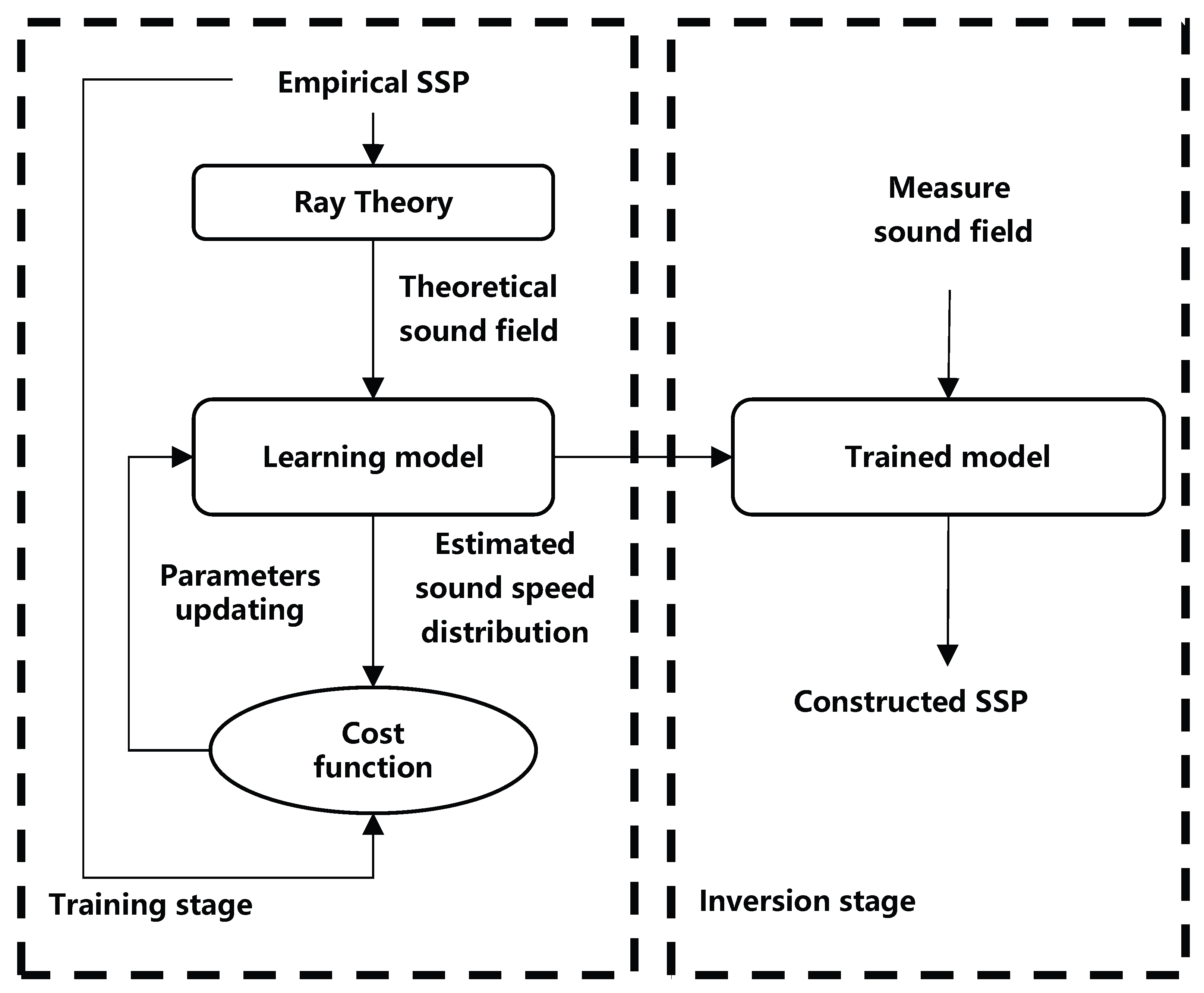
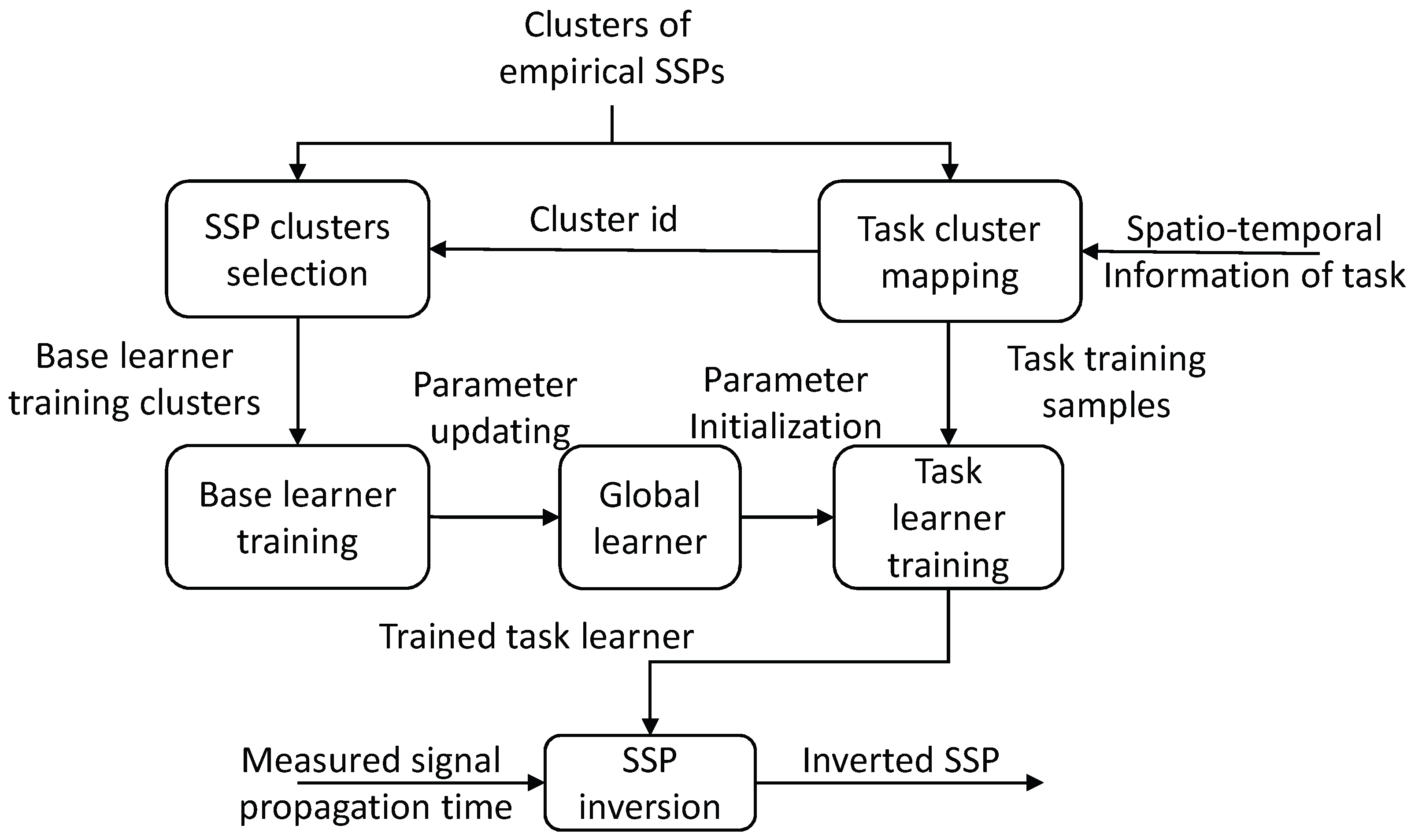
3.3. DL for SSP Inversion

3.3.1. Neural Network Inversion of SSP Based on Sound Field Observation Data

In recent years, machine learning has been widely applied in regression and classification problems in multiple fields such as image recognition and numerical prediction. Benefiting from its ability to fit complex nonlinear relationships, it is very suitable for solving the problem of inversion of sound speed distribution from sound field distribution. In 1995, Stephan first established a framework for inversion of sound speed fields using artificial neural networks (ANNs) [49], as shown in Figure 5.

The main idea of deep learning ANN for constructing SSPs is to invert the SSP by mining the implicit sound speed distribution information in the sound field data. For empirical SSP samples, under the condition of known topological relationships between the signal source and receivers, sound field simulation is carried out using normal mode theory, ray theory, or parabolic equation models. The simulated sound field information is used as input data for the model, and the labeled values of the SSP are used as output. During the training stage, the model’s parameters are adjusted according to established cost functions, which establishes a mapping relationship from sound field to sound speed field. At the inversion stage, by putting real-time measured sound field information into the model, the SSP of the target area can be constructed.

The distribution of sound speed has spatial and temporal differences, and the advantage of deep learning ANN models for constructing SSPs is that specialized models can be pre-set for different spatial and temporal intervals during model establishment. Then, the training of the model can be completed offline in advance. After model convergence, for inputting sound field data, only one turn of forward iteration matrix operation is required to obtain the estimated SSP. Therefore, compared to MFP-based and CS-based SSP inversion methods, its inversion stage has significant real-time advantages. However, the ANN model also faces two important challenges when used to construct SSPs. On the one hand, underwater sound field measurement is inevitably affected by complex underwater environmental coupling interference, such as noise and multipath effects, which will reduce the accuracy of the model. On the other hand, ANN model training requires a large number of empirical SSPs as reference data samples. Due to the high cost of obtaining empirical SSP data through instruments such as CTD or SVP, there are problems of insufficient training sample data in many ocean areas, which can easily lead to accuracy performance decreasing due to the overfitting phenomenon.

In order to improve the robustness of DL-based SSP construction models against noise in sound field measurement, we proposed an auto-encoding feature mapping neural network (AEFMNN) structure in 2021 [50], as shown in Figure 6. By using an auto-encoding neural network to reconstruct noisy sound fields into denoised sound fields, stronger, more robust hidden features are extracted. Then, the feature mapping network is used to establish a mapping relationship from hidden features to the distribution of SSPs.

To address the problem of overfitting in few-shot learning scenarios, we proposed an ANN model for SSP construction with an intelligent extended dataset [51] based on [50]. This method first extracts feature points from existing reference samples and then generates new SSP samples based on the extracted feature points to expand the reference sample dataset (the expanded samples do not exceed $30\%$ of the total samples). This method to some extent alleviates the situation of insufficient reference sample data but still has certain requirements for the amount of original reference sample data.

In order to effectively address the overfitting effect in few-shot learning, in 2023, reference [52] proposed a task-driven meta-learning (TDML) framework for constructing SSPs. The model is shown in Figure 7. TDML includes multiple base learners, a global learner, and on-demand task learners. The core idea is to use multiple base learners to simultaneously learn different spatio–temporal regions and types of SSPs, obtain common features of SSP distribution, and pass them on to the task learner, enabling the task learner to achieve model convergence with a small number of samples and training. Through this process, the sensitivity of the model to input data can be maintained, thereby improving its ability to cope with overfitting.

The model training method of TDML is shown in Figure 8. During the meta-model (the base learners and the global learner) training stage, for each round of parameter updating, K samples are randomly selected from a set of A SSP types and assigned to K base learners one by one. Each base learner uses N samples for training and one sample for testing. This training method is called K-way N-shot.

The aforementioned ANN, AEFMNN, and TDML methods for SSP inversion all use neural network models to establish a mapping relationship from sound field to sound speed distribution, which can quickly estimate the distribution of SSPs based on real-time sound field input data. However, due to the economic costs of device development and limited coverage range, these methods, similar to traditional MFP and CS methods, have spatial constraints on their applications.

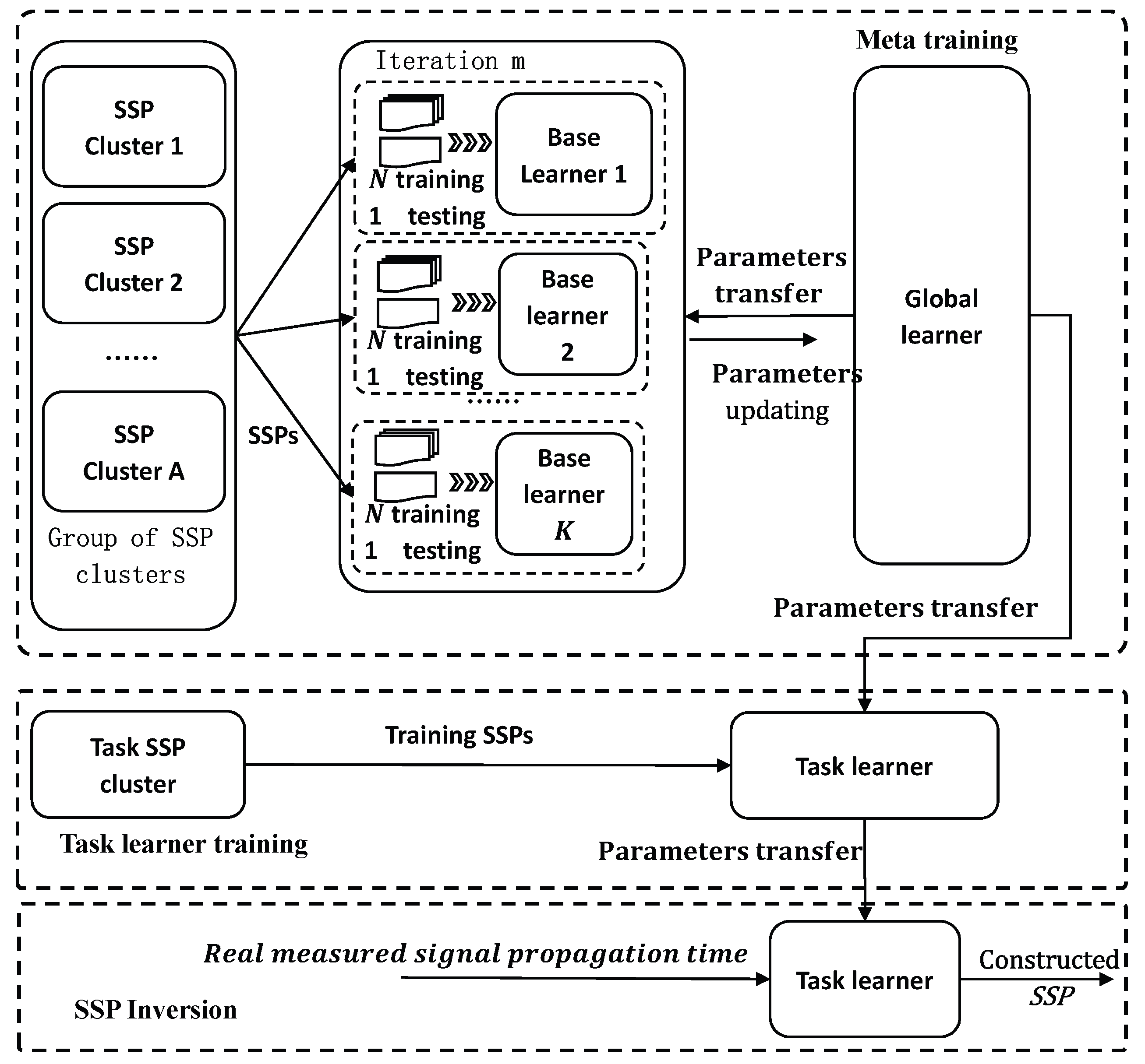
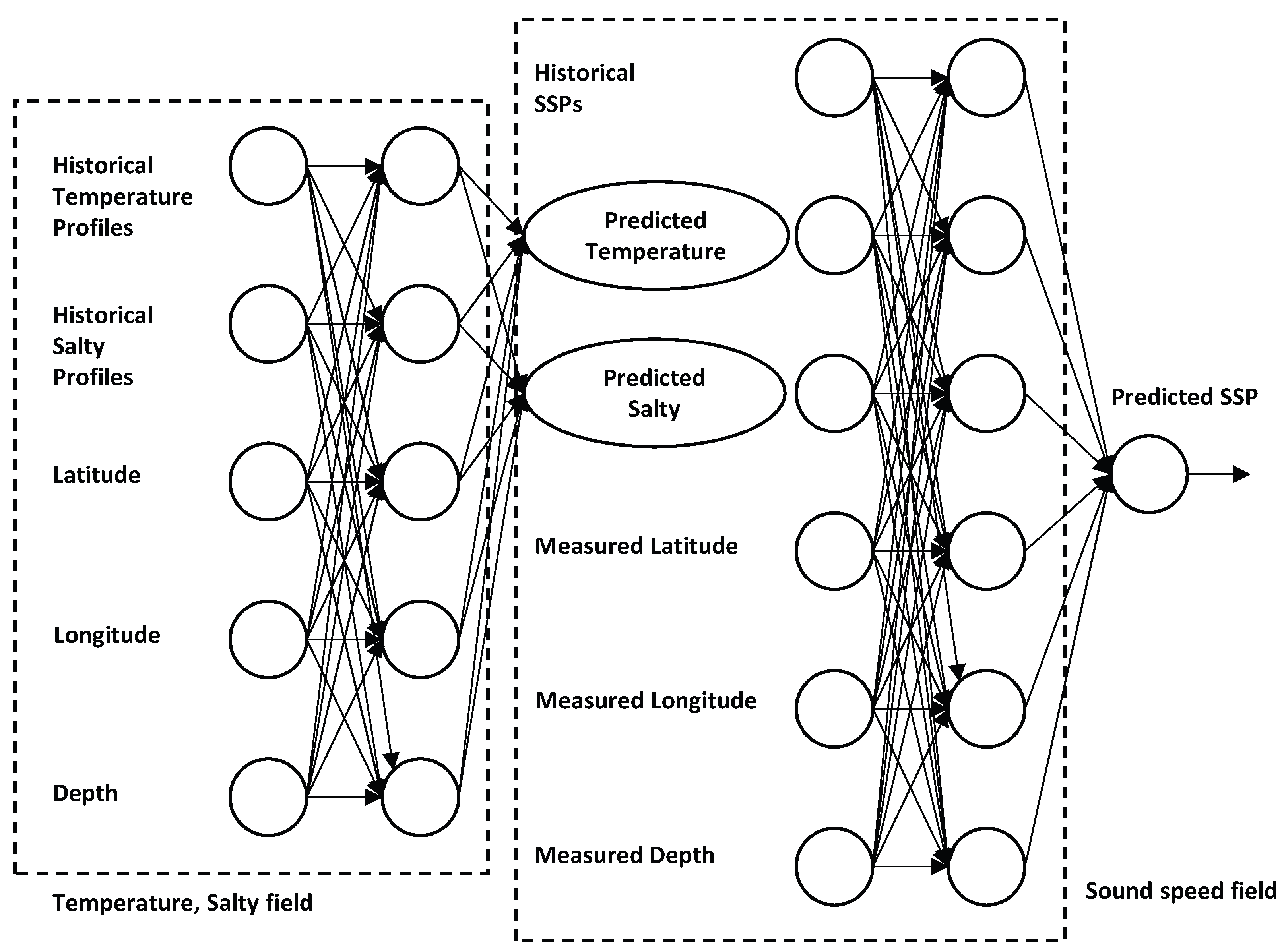
3.3.2. Constructing SSPs Using Neural Networks Without Sound Field Observation Data

In order to construct an SSP in a spatio–temporal interval without obtaining sound field observation data, reference [50] provides a strategy for constructing a large-scale three-dimensional sound speed field using multiple base stations in different regions. The application scenario of reference [50] is for a distributed seabed observation system, where multiple pairs of buoys or anchors with relatively concentrated spatial orientations form a base station group (which can communicate with each other internally). By measuring the sound field at each base station group, the SSP of the base station group area is inverted. After inverting the SSPs of multiple base station groups, the three-dimensional sound distribution of the whole area can be obtained through interpolation. Ultimately, the sound speed field within the closed area of the base station group can be constructed, although it does not reduce equipment development costs.

In 2020, Yu et al. [53] and Wang [54] proposed a SSP prediction method based on a radial basis function (RBF) neural network. The model structure is shown in Figure 9. This method sets up a network for constructing temperature and salinity fields, as well as a network for constructing sound speed fields. Firstly, it utilizes historical temperature and salinity profiles and their sampling longitude, latitude, and depth information to construct the average temperature and salinity fields in the target area, providing constraints for constructing a network for SSPs. Secondly, the average SSP of the target area is constructed using the historical SSP and its sampling longitude, latitude, and depth information. The RBF method does not require on-site measurement of sound field observation data, but the model construction results tend to approach the mean of regional samples, making it difficult to accurately describe the temporal and spatial distribution changes in SSPs.

In 2022, Li proposed a full-ocean-depth SSP inversion method based on the self-organizing map (SOM) neural network [55]. The model structure is shown in Figure 10. This method fully utilizes empirical SSP data and ocean surface temperature data observed from the global satellite remote sensing system and optionally incorporates ocean surface sound speed measurement data, providing a feasible solution for constructing SSPs without sound field observation data. Compared to the SSP estimation method based on RBF neural networks, it can construct different spatial sound speed distributions to better reflect the spatial differences in sound speed distribution. But due to the model’s reliance on ocean surface temperature and sound speed data, it is not possible to fully describe the distribution of sound speed in the seasonal thermocline. Therefore, there is still great space for improvement in the accuracy of constructing the full-ocean-depth SSP.

3.3.3. Typical Sound Field Measurement Mode

In the framework of MFP, CS, and DL for SSP inversion, the accuracy of using sound field observation data for sound speed field inversion is still higher than that without sonar observation data at present. In terms of sound field information measurement, the Scripps Institute of Oceanography of the United States early adopted a single input, single output (SISO) system for sound field measurement, using multipath signals to invert the environmental sound speed distribution [35]. In order to increase the information content of sound field data measurement and reduce the impact of environmental noise on measurement accuracy, the US Navy Laboratory used a single input multiple output (SIMO) system [36] to validate the MFP sound speed inversion algorithm, which is implemented in the form of a ship-towed vertical array as shown in Figure 11a.

The Institute of Acoustics, Chinese Academy of Sciences, has proposed a method of using seabed horizontal arrays for MFP to invert SSPs in response to the unstable attitude of vertical arrays and successfully obtained shallow water sound speed inversion results [56,57], as shown in Figure 11b. However, due to the difficulty in recycling and reusing seabed arrays, the economic cost of equipment production is high.

4. Comparison of Methods for Constructing Underwater SSPs

Table 3. Comparison of different methods for constructing underwater SSPs.

Method	Sonar Data	Accuracy	Time Consumption		Advantage	Disadvantage
			Preparation	Construction
CTD/SVP [20,21,22,23,24,26]	no	high	-	very long	accurate	very long period; high economic costs
XCTD [25,27,28,29,30]	no	high	-	long	accurate; portable	long period; limited depth coverage
EOF-MFP [36,37,38,39,40,41,42,43,44]	yes	good	very short	medium	near real-time	complex optimization object searching
Dictionary learning [45,46]	yes	good	short	medium	near real-time	complex optimization object searching
CS [47,48]	yes	medium	short	short	sparse representation low storage space; not bad real-time	accuracy loss by linear representation
ANN [49,51]	yes	good	long	very short	real-time	complex preparation stage; weak noise reistance; overfitting problem
AEFMNN [50]	yes	good	long	very short	real-time; good robustness	complex preparation stage; overfitting problem
TDML [52]	yes	good	very long	very short	real-time; anti-overfitting	complex preparation stage
RBF [53,54]	no	low	long	very short	real-time; no sonar data	weak time and space resolution ability
SOM [55]	no	low	long	very short	real-time; no sonar data	insufficient accuracy in the deep-ocean part and seasonal thermocline

summarizes the basic attributes of different methods for constructing SSPs. The construction accuracy is divided into high, good, medium, and low levels from the best to the worst. The time cost is divided into the preparation phase and the inversion phase, and the preparation phase can be completed offline. Therefore, the time cost performance of the inversion phase is more critical and is divided into five levels from the best to the worst: very short, short, medium, long, and very long. Due to the fact that CTD, SVP, XCTD, and other devices belong to direct measurement methods, their time costs are calculated in hours and minutes, while MFP, CS, and DL models belong to sound speed inversion methods, and their time costs are usually calculated in minutes and seconds. Therefore, the “very long, long” levels of time cost are much greater than the “medium, short, and very short” levels of time cost.

Through comparison, it can be seen that the biggest advantage of the direct measurement method lies in its accurate measurement results, which can usually be considered as true values. The main disadvantage is that the measurement period is long, and it is difficult to meet the real-time requirements for estimating the sound speed distribution in underwater applications. In the SSP inversion methods, the construction of SSPs using sound field observation data has higher accuracy than the case without sound field observation data. Compared to MFP, CS improves real-time performance but sacrifices accuracy. Compared to the two methods mentioned above, the neural network model performs better in accuracy and real-time performance, but in essence, its real-time advantage is at the cost of sacrificing the time cost of the preparation stage. The biggest advantage of RBF and SOM models is that they are not constrained by sound field observation data, making them widely applicable to various regions around the world and greatly reducing the cost of underwater acoustic equipment. However, after training with designated spatio–temporal data, the generalization ability of RBF models in time and space resolution is insufficient, while the fitting accuracy of SOM models for seasonal thermocline and deep-sea isothermal layer is insufficient.

With the development of underwater sensing technology, robotics technology, and the long-term accumulation of empirical observation data, the overall trend of SSP construction methods is towards intelligence, real-time, and precision. On the one hand, the increase in data sources means that the selectivity of methods for constructing sound speed fields is improved. In different regions, elastic construction of sound speed fields based on the available data sources will be an excellent solution to meet the accuracy or real-time requirements of underwater users for estimating sound speed distribution in the future. On the other hand, in the absence of sound field observation data, how to use historical observation data and prior information, which can be quickly measured through remote sensing or sea surface, to intelligently and accurately construct a full ocean depth sound speed field is still a research point worth further exploration.

5. Conclusions

This paper introduces and investigates the current research status of underwater sound speed field construction, which can be divided into two categories: direct measurement methods and sound speed inversion methods. For direct measurement methods, this paper investigates and lists the current mainstream commercial equipment and instruments and lists their main performance parameters. For sound speed inversion methods, this paper summarizes the three major frameworks of MFP, CS, and DL based on the principles for constructing sound speed fields. By analyzing the principles of specific methods within each framework, the advantages and disadvantages of different sound speed field construction methods are compared, and the evolution trend of sound speed field construction methods is summarized, which is towards intelligent, real-time, and accurate development. The existing real-time construction methods for sound speed fields do not match the ability of sound field data observation, which limits the universality of underwater sound speed inversion methods. Therefore, how to use limited prior information for intelligent and high-precision construction of full-ocean-depth sound speed fields in the absence of sound field observation data is a major trend in future research. In addition, how to use multi-source observation data to provide elastic estimation services for underwater users with different accuracy and real-time requirements of sound speed distribution is another important trend in future research. The work of this paper will provide reference for subsequent research on the construction of underwater sound speed fields.

References

1. Lin, B.; Zhang, Z.; Han, X.; Liu, L.; Liu, Z.; Che, Y. Key Technologies for Space-Air-Ground-Ocean Integrated Networks towards Maritime Emergency: An Overview. Mob. Commun. 2020, 44, 19–26. [Google Scholar]
2. Jensen, F.B.; Kuperman, W.A.; Porter, M.B.; Schmidt, H. Computational Ocean Acoustics: Chapter 1; Springer Science & Business Media: Berlin/Heidelberg, Germany, 2011; pp. 3–4. [Google Scholar] [CrossRef]
3. Munk, W.; Wunsch, C. Ocean acoustic tomography: A scheme for large scale monitoring. Deep. Sea Res. Part Oceanogr. Res. Pap. 1979, 26, 123–161. [Google Scholar] [CrossRef]
4. Munk, W.; Wunsch, C. Ocean acoustic tomography: Rays and modes. Rev. Geophys. 1983, 21, 777–793. [Google Scholar] [CrossRef]
5. Munk, W.; Worcester, P.; Wunsch, C. Ocean Acoustic Tomography; Cambridge University Press: Cambridge, UK, 1995. [Google Scholar]
6. Lasky, M. Review of undersea acoustics to 1950. J. Acoust. Soc. Am. 1977, 61, 283–297. [Google Scholar] [CrossRef]
7. Overview of the Development of Ocean Survey Instruments Abroad. Mar. Sci. Technol. Inf. 1977, 5, 24–44. (In Chinese)
8. Wilson, D.W. Equation for the Speed of Sound in Sea Water. J. Acoust. Soc. Am. 1977, 32, 1357. [Google Scholar] [CrossRef]
9. Wang, D.; Shang, E. Marine Acoustic; China Science Publishing and Media Ltd. (CSPM): Beijing, China, 2013. (In Chinese) [Google Scholar]
10. Zhang, L.; Ye, S.; Zhou, S.; Liu, F.; Han, Y. Review of Measurement Techniques for Temperature, Salinity and Depth Profile of Sea Water. Mar. Sci. Bull. 2017, 36, 481–489. (In Chinese) [Google Scholar]
11. Claude, L.C. Development of Simple Equations for Accurate and More Realistic Calculation of the Speed of Sound in Seawater. J. Acoust. Soc. Am. 1969, 46, 216–226. [Google Scholar]
12. Medwin, H. Speed of sound in water: A simple equation for realistic parameters. J. Acoust. Soc. Am. 1975, 58, 1318–1319. [Google Scholar] [CrossRef]
13. Del-Grosso, V.A. New equation for the speed of sound in natural waters (with comparisons to other equations). J. Acoust. Soc. Am. 1974, 56, 1084. [Google Scholar] [CrossRef]
14. Chen, C.T.; Millero, F.J. Speed of sound in seawater at high pressures. J. Acoust. Soc. Am. 1977, 62, 1129–1135. [Google Scholar] [CrossRef]
15. Huang, C.; Lu, X.; Wang, K.; Shen, J.; Zhang, B.; Zhai, G. A method of exactly determining the sound velocity in deep water based on salt information from WOA13 model and XBT data. Mar. Sci. Bull. 2016, 35, 554–561. [Google Scholar]
16. Millero, F.J.; Li, X. Comments on "On equations for the speed of sound in sea water". J. Acoust. Soc. Am. 1994, 93, 255–275. [Google Scholar]
17. Coppens, B.A. Simple equations for the speed of sound in Neptunian waters. J. Acoust. Soc. Am. 1981, 69, 862–863. [Google Scholar] [CrossRef]
18. Zhou, F.; Zhao, J.; Zhou, C. Determination of the Optimal Sound Velocity Formula for Multibeam Sounding Systems. J. Ocean. Phy. Taiwan Strait. 2001, 4, 411–419. [Google Scholar]
19. Chen, C.; Wu, B.; Wang, S. Research on optimization selection of computation formulas for underwater sound velocity. Ship Sci. Technol. 2014, 36, 77–80. [Google Scholar]
20. Sea-Bird Scientific. SBE CTDs Profiling. Available online: https://www.seabird.com/profiling/family?productCategoryId=54627473767 (accessed on 12 December 2023).
21. YSI, Inc. SonTek CastAway-CTD. Available online: https://www.ysi.com/castaway-ctd (accessed on 12 December 2023).
22. Ocean Seven Ocean Seven 320 Plus WOCE-CTD. Available online: https://www.idronaut.it/multiparameter-ctds/oceanographic-ctds/os320plus-oceanographic-ctd/ (accessed on 12 December 2023).
23. RBR, Ltd. RBR CT and CTD Instruments. Available online: https://rbr-global.com/support/documentation/ (accessed on 12 December 2023).
24. Sea & Sun Technology, GmbH. Sea & Sun Technology CTD Probes. Available online: https://www.sea-sun-tech.com/product-category/probes/ctd-probes/ (accessed on 12 December 2023).
25. Tsurumi-Seiki Co., L. eXpendable Conductivity, Temperature and Depth Product Code: XCTD. Available online: https://tsurumi-seiki.co.jp/en/product/e-sku-2/ (accessed on 12 December 2023).
26. Ocean Physics Technology. OST Series CTD. Available online: https://www.oceanphysics.cn/index.php?a=shows&catid=69&id=81 (accessed on 12 December 2023).
27. Trampp, D.A. Upper Ocean Characteristics in the Tropical Indian Ocean from AXBT and AXCTD Measurements; Technical Report; Naval Postgraduate School: Monterey, CA, USA, 2012. [Google Scholar]
28. Shi, X.; Su, Q. Development Status of Expendable Marine Instruments and Equipment. Acoust. Electron. Eng. 2015, 4, 46–48. [Google Scholar]
29. Cheng, F.; Chen, S.; Jin, S.; Sun, W. An Expanding Method of Sound Velocity Profiles Via EOF in Marginal Deepwater Areas. Hydrogr. Surv. Charting 2016, 36, 26–29. (In Chinese) [Google Scholar]
30. Huang, W.; Lu, J.; Li, S.; Xu, T.; Wang, J.; Zhang, H. Fast Estimation of Full Depth Sound Speed Profile Based on Partial Prior Information. In Proceedings of the 2023 IEEE 6th International Conference on Electronic Information and Communication Technology (ICEICT), Qingdao, China, 21–24 July 2023; IEEE: Piscataway, NJ, USA, 2023; pp. 479–484. [Google Scholar] [CrossRef]
31. AML Oceanographic Ltd. MVP300 Operation and Maintenance Manual. Available online: https://amloceanographic.com/moving-vessel-profiler-for-uncrewed-systems-vessels (accessed on 12 December 2023).
32. Wang, Y.; Yi, X. A Towed Multi-parameter Profile Measurement System. Oceanography; Technical report; CNKI: Beijing, China, 2005. [Google Scholar]
33. Products, D.U.T. CZT1-3A Towed Multi-Parameter Profile Measurement System. 715 Research Institute of China: Hangzhou, China, 2010. [Google Scholar]
34. Ren, Q.; Yu, F.; Wei, C.; Tang, Y.; Lu, N. Development and Application of A Moving Multi-parameter Profile Measurement System. Hydrogr. Surv. Charting 2022, 42, 33–36. (In Chinese) [Google Scholar]
35. Cornuelle, B.; Munk, W.; Worcester, P. Ocean acoustic tomography from ships. J. Geophys. Res. Ocean. 1989, 94, 6232–6250. [Google Scholar] [CrossRef]
36. Tolstoy, A.; Diachok, O.; Frazer, L. Acoustic tomography via matched field processing. J. Acoust. Soc. Am. 1991, 89, 1119–1127. [Google Scholar] [CrossRef]
37. Zhang, Z. A Study on Inversion for Sound Speed Profile in Shallow Water (in Chinese). Ph.D. Thesis, Northwestern Polytechnical University, Xi’an, China, 2002. [Google Scholar]
38. Zhang, W.; Yang, S.e.; Huang, Y.w.; Li, L. Inversion of sound speed profile in shallow water with irregular seabed. In Proceedings of the Advances in Ocean Acoustics: Proceedings of the 3rd International Conference on Ocean Acoustics (OA2012), Beijing, China, 21–25 May 2012; 1495; AIP: Melville, NY, USA, 2012; pp. 392–399. [Google Scholar] [CrossRef]
39. Zhang, W. Inversion of Sound Speed Profile in Three-dimensional Shallow Water. Ph.D. Thesis, Chapter 2. Harbin Engineering University, Harbin, China, 2013. (In Chinese). [Google Scholar]
40. Zheng, G.Y.; Huang, Y.W. Improved Perturbation Method for Sound Speed Profile Inversion. J. Harbin Eng. Univ. 2017, 38, 371–377. [Google Scholar] [CrossRef]
41. Zhang, Z.M. The Study for Sound Speed Inversion in Shallow Water on Application of Genetic and Simulated Annealing Algorithms. Master’s Thesis, Chapter 4. Harbin Engineering University, Harbin, China, 2005. [Google Scholar] [CrossRef]
42. Tang, J.F.; Yang, S.E. Sound speed profile in ocean inverted by using travel time. J. Harbin Eng. Univ. 2006, 27, 733–737. [Google Scholar] [CrossRef]
43. Sun, W.C.; Bao, J.Y.; Jin, S.H.; Xiao, F.M.; Cui, Y. Inversion of Sound Velocity Profiles by Correcting the Terrain Distortion. Geomat. Inf. Sci. Wuhan Univ. 2016, 41, 349–355. [Google Scholar] [CrossRef]
44. Zhang, M.; Xu, W.; Xu, Y. Inversion of the sound speed with radiated noise of an autonomous underwater vehicle in shallow water waveguides. IEEE J. Ocean. Eng. 2015, 41, 204–216. [Google Scholar] [CrossRef]
45. Bianco, M.; Gerstoft, P. Dictionary learning of sound speed profiles. J. Acoust. Soc. Am. 2017, 140, 1749–1758. [Google Scholar] [CrossRef]
46. Bianco, M.; Gerstoft, P.; Traer, J.; Ozanich, E.; Roch, M.A.; Gannot, S.; Deledalle, C.A. Machine learning in acoustics: Theory and applications. J. Acoust. Soc. Am. 2019, 146, 3590–3628. [Google Scholar] [CrossRef]
47. Bianco, M.; Gerstoft, P. Compressive Acoustic Sound Speed Profile Estimation. J. Acoust. Soc. Am. 2016, 139, EL90–EL94. [Google Scholar] [CrossRef]
48. Choo, Y.; Seong, W. Compressive sound speed profile inversion using beamforming results. Remote Sens. 2018, 10, 704. [Google Scholar] [CrossRef]
49. Stephan, Y.; Thiria, S.; Badran, F. Inverting Tomographic Data with Neural Nets. In Proceedings of the Challenges of Our Changing Global Environment, San Diego, CA, USA, 9–12 October 1995; IEEE: Piscataway, NJ, USA, 1995; pp. 1501–1504. [Google Scholar]
50. Huang, W.; Liu, M.; Li, D.; Yin, F.; Chen, H.; Zhou, J.; Xu, H. Collaborating Ray Tracing and AI Model for AUV-Assisted 3-D Underwater Sound-Speed Inversion. IEEE J. Ocean. Eng. 2021, 46, 1372–1390. [Google Scholar] [CrossRef]
51. Huang, W.; Li, D.; Jiang, P. Underwater Sound Speed Inversion by Joint Artificial Neural Network and Ray Theory. In Proceedings of the Proceedings of the Thirteenth ACM International Conference on Underwater Networks & Systems (WUWNet’18), Shenzhen, China, 3–5 December 2018; ACM: New York, NY, USA, 2018; pp. 1–8. [Google Scholar] [CrossRef]
52. Huang, W.; Li, D.; Zhang, H.; Xu, T.; Yin, F. A meta-deep-learning framework for spatio-temporal underwater SSP inversion. Front. Mar. Sci. 2023, 10. [Google Scholar] [CrossRef]
53. Yu, X.; Xu, T.; Wang, j. Sound Velocity Profile Prediction Method Based on RBF Neural Network. In Proceedings of the In Proceedings of China Satellite Navigation Conference (CSNC), Chengdu, China, 23–25 May 2020; Springer: Berlin/Heidelberg, Germany, 2020; pp. 1–8. [Google Scholar]
54. Wang, J. Research on Theory and Method of Marine Precise Acoustic Data Processing. Ph.D. Thesis, Shandong University, Weihai, China, 2022. (In Chinese). [Google Scholar]
55. Li, Q.; Shi, J.; Zhenglin, L.; Yu, L.; Zhang, K. Acoustic sound speed profile inversion based on orthogonal matching pursuit. Acta Oceanol. Sin. 2022, 38, 149–157. [Google Scholar] [CrossRef]
56. Li, F.; Zhang, R. Inversion for sound speed profile by using a bottom mounted horizontal line array in shallow water. Chin. Phys. Lett. 2010, 27, 084303. [Google Scholar] [CrossRef]
57. Li, Z.; He, L.; Zhang, R.; Li, F.; Yu, Y.; Lin, P. Sound speed profile inversion using a horizontal line array in shallow water. Sci. China Phys. Mech. Astron. 2015, 58, 1–7. [Google Scholar] [CrossRef]
Figure 1. Typical commercial CTDs and XCTDs. (a) SBE 911 plus by Sea Bird Inc. (b) OS 320 plus by Idronaut. (c) XCTD by TSK. (d) OST by National Ocean Technology Center of China.
Jmse 12 02356 g001
Figure 2. Ship-assisted SSP measurement. (a) CTD. (b) XCTD.
Jmse 12 02356 g002
Figure 3. MFP framework for SSP inversion.
Jmse 12 02356 g003
Figure 4. CS framework for SSP inversion.
Jmse 12 02356 g004
Figure 5. DL framework for SSP inversion.
Jmse 12 02356 g005
Figure 6. AEFMNN model for SSP inversion.
Jmse 12 02356 g006
Figure 7. TDML model for SSP inversion.
Jmse 12 02356 g007
Figure 8. Training and inversion of SSP based on TDML model.
Jmse 12 02356 g008
Figure 9. RBF model for SSP inversion.
Jmse 12 02356 g009
Figure 10. SOM model for SSP inversion.
Jmse 12 02356 g010
Figure 11. Sound field data measurement. (a) Vertical array. (b) Horizontal array.
Jmse 12 02356 g011