Stratification Effects on Estuarine Mixing: Comparative Analysis of the Danshui Estuary and a Thermal Discharge Outlet

Abstract

Estuaries serve as transitional zones between rivers and the ocean, and their mixed dynamic characteristics are crucial for the transport, transformation, and cycling of materials. This study investigates the mixing characteristics and their dominant factors in the Danshui Estuary and thermal discharge outlets through field measurements. Based on CTD (Conductance Temperature Depth) profiles and nutrient concentration measurements, the Danshui Estuary exhibited significant stratification during the October 2016 cruise, while vertical mixing was uniform during the March 2017 cruise. Vertical mixing was suppressed during stratification, but the nutrient concentration varied with salinity in a manner that was similar to non-stratified conditions, generally conforming to the theoretical dilution curve, which means physical mixing dominated here, indicating that horizontal mixing is predominant in the Danshui Estuary. The spatial scale calibrated horizontal dispersion coefficients were measured as 9.16 ± 1.57 m² s⁻¹ and 11.84 ± 1.71 m² s⁻¹ for stratified and non-stratified conditions, respectively, highlighting the Danshui Estuary’s strong horizontal mixing. Thermal discharge outlets are an important type of estuarine environment in non-natural estuaries. The 3D thermohaline structure measured by the underway CTD revealed an upwelling of cold and high-salinity water during the flood tide. The calculated Richardson number during the flood tide was approximately 0.7, indicating a very strong stratification effect. The horizontal dispersion coefficients calibrated by spatial scale showed no significant difference between different tides (flood tide: 0.53 ± 0.18 m² s⁻¹, ebb tide: 0.46 ± 0.17 m² s⁻¹). Therefore, the slower temperature decay during the flood tide, as reflected by the e-folding time (flood tide: 4.19 ± 2.33 min, ebb tide: 2.14 ± 0.40 min), is attributed to the strong stratification. Based on these findings, it is recommended that the power plant mitigates the impact of waste heat on the marine environment by increasing discharge during the ebb tide and reducing it during the flood tide.

1. Introduction

Terrestrial materials, delivered to the marine environment via surface runoff and groundwater, significantly impact coastal marine ecosystems. These materials accumulate and disperse within the coastal ocean and ultimately enter offshore waters through the oceanic currents. The concentration of terrestrial materials at the land–sea interface profoundly influences the coastal environment and marine ecosystems. In coastal waters, these materials undergo transport and mixing processes. The physical effects of mixing on material concentration are considerably more significant than the biochemical interactions among substances [1]. Consequently, estimating the efficiency of mixing in coastal and estuarine environments, as well as monitoring and understanding its temporal and spatial variations, is central to the assessment and management of coastal environments.

The mixing rate of coastal materials is influenced by a variety of factors, including bathymetry, wave action, and processes [1,2]. These factors exhibit high spatial–temporal variability, posing a significant challenge in estimating actual coastal mixing efficiency. Additionally, estuaries often experience stratification due to the substantial density difference between freshwater and surrounding seawater. These vertical stratified structures further suppress turbulence intensity. Understanding the balance between stratification and turbulence is not only a crucial topic in environmental fluid dynamics research, but also holds significant value for coastal management applications, such as the environmental issue of coastal hypoxia.

Since the advent of the Hubble ammonia process, which marked the beginning of artificial nitrogen fixation, the amount of artificially fixed nitrogen has been steadily increasing [3]. By the 1980s, it had even surpassed the total amount of natural nitrogen fixation [4]. The use of nitrogen fertilizers to boost crop yields has led to an accumulation of nitrogen in estuaries, transported by river runoff, exerting environmental pressure on estuarine waters and resulting in eutrophication and hypoxia. For instance, in the Yangtze Estuary, the content of nitrogen compounds in 2003 had tripled compared to 1970 [5,6]. If nutrients are not diluted promptly, coastal waters can deteriorate into dead zones, leading to the death of a large number of aquatic organisms and potentially causing a loss of resistance and resilience in regional ecosystems.

In the 1970s, dead zones were predominantly observed in developed countries. However, by 2010, their presence had expanded globally, with an exponential increase in the number of ecosystems affected by this phenomenon [7]. The global average input of terrestrial DIN (dissolved inorganic nitrogen) is approximately 208 kg N km⁻² year⁻¹ [8]. Notably, the DIN load of the Danshui River, the largest river in northern Taiwan, reaches as high as 8020 kg N km⁻² year⁻¹, which is 39 times the global average [9]. Under these conditions of nutrient enrichment, the role of estuarine mixing becomes a matter of critical importance.

It has also been recognized that society can impact estuarine processes by altering the thermal regime. Nuclear power plants lose 68% of their heat during the energy conversion process [10], with a substantial amount of heat being discharged into the coastal ocean. The warm water significantly alters the temperature structure of the receiving water, impacting water quality and marine ecological processes in a manner analogous to terrestrial nutrients. The Third Nuclear Power Plant, located on the Hengchun Peninsula at the southernmost tip of Taiwan in Nanwan Bay, is in an area renowned for its beautiful corals. To protect the nearby corals, the plant invested heavily during construction in equipment to mitigate the thermal discharge impact. This site offers an ideal location for studying mixing mechanisms in estuarine areas, with thermal discharge as the focal point of study.

The purpose of this study is to investigate the mixing mechanisms of terrestrial materials, specifically DIN and thermal discharge, within estuarine environments. We focus on the interactions between these materials and the marine hydrodynamic environment. By examining the mixing and dispersion processes of terrestrial materials, this work sheds light on the dynamics that drive coastal eutrophication, hypoxia, and the formation of dead zones. The findings are essential for developing strategies to mitigate environmental pressures on estuarine ecosystems, especially in regions with high nutrient loading such as the Danshui River. Furthermore, the study is expected to provide a unique perspective on the impacts of thermal pollution on coral reefs, which is critical for conservation efforts.

2. Materials and Methods

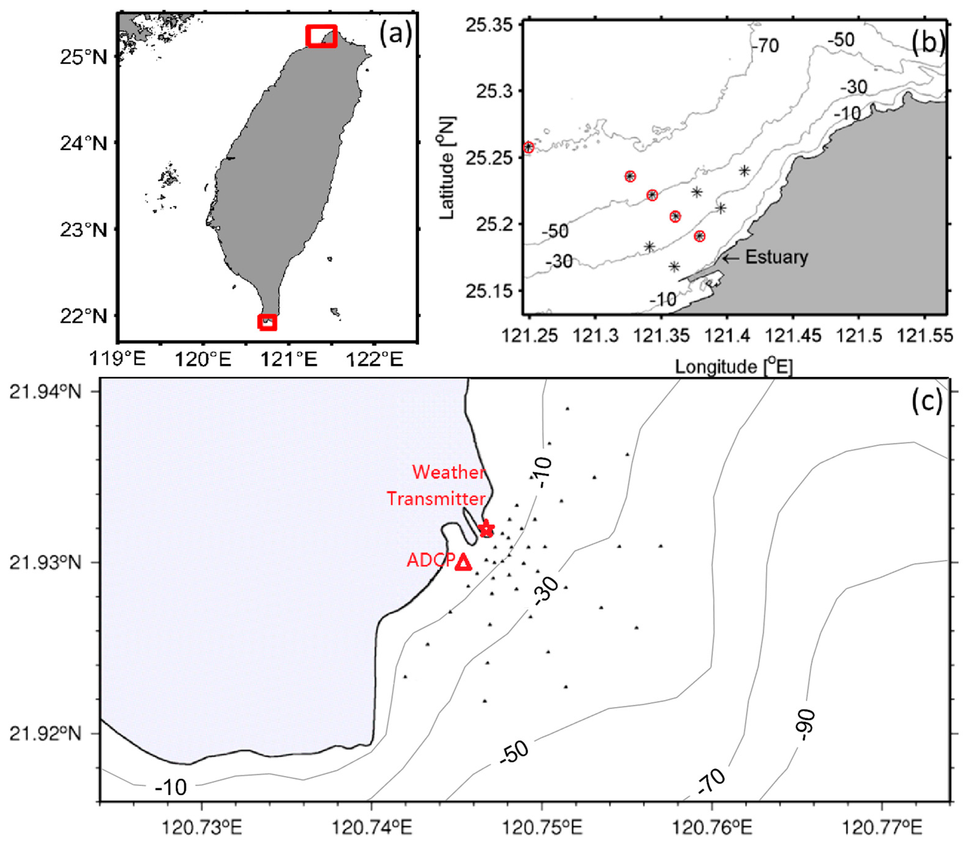
2.1. Study Area

The study focused on two distinct regions in Taiwan: the Danshui Estuary in the northwest and the thermal discharge area associated with the Third Nuclear Power Plant in the south (Figure 1a). The Danshui Estuary serves as a representative large-scale ecosystem, spanning approximately 20 km and exhibiting seasonal dynamics, with its surrounding bathymetric features depicted in Figure 1b. The Danshui River, measuring 158.7 km in length, originates from Mount Pin-Tian at an elevation of 3529 m above sea level and drains a basin covering 2726 km². Precipitation in the upper reaches of the Danshui River can peak at 3000–4000 mm annually, while, in the estuary, it averages around 2000 mm, with minimal seasonal fluctuation. The river’s annual average discharge is approximately 210 m³ s⁻¹, and the mean annual temperature is around 22 °C [11]. Forest cover predominates across the entire watershed of the Danshui River, with a gradual decrease in percentage from nearly 97% in the upper reaches to about 75% in the lower reaches [12].

The thermal discharge area of the nuclear power plant serves as an example of a small-scale ecosystem (~1 km and tidal time scale). As shown in Figure 1c, the outlet is oriented towards the southeast. The predominant tidal pattern in this region is a combination of diurnal and semi-diurnal components. The tidal current, which varies from 0.2 to 0.4 m/s, flows southwestward during the flood tide and northeastward during the ebb tide. Jan et al. [13] documented a persistent southwestward sub-tidal flow around the thermal discharge outlet, with an average velocity of 0.15 m s⁻¹. They also noted an abrupt decrease in temperature at a distance of 200 m from the outlet. The surrounding area, with water depths ranging from 6 m to 30 m, is rich in corals distributed across the rocky seabed.

2.2. Measuring Method

For the Danshui Estuary, CTD measurements (SBE37-CTD, Sea-Bird Electronics Co., Ltd., Washington, DC, USA) and water sample collections were conducted across different seasons by Ocean Research Vessel No.2 (ORII, operated by the National Taiwan Ocean University, Keelung, Taiwan). In the thermal discharge area of the nuclear power plant, underway CTD (UCTD, UCTD 10-400, Oceanscience Group, Oceanside, CA, USA) and thermometers mounted on sea surface drifters (self-developed) were utilized for three-dimensional observations, and the rate of temperature decay of water masses was quantitatively assessed using heat as a tracer.

2.2.1. CTD Measurement

The CTD data include conductivity (S m⁻¹), temperature (°C), pressure (dbar), descent rate (m s⁻¹), and salinity (PSU). The CTD measurements within the Danshui Estuary were executed by ORII on 5 October 2016 and 22 March 2017, respectively. All the ten measuring sites indicated as asterisks in Figure 1b were distributed evenly across the potential influence zone of the estuarine plume.

In the thermal discharge area of the nuclear power plant, UCTD observations were conducted on 20 April 2017 using a small fishing boat, at all 43 sampling points (dots in Figure 1c). All the points spread evenly in a fan-shaped pattern around the thermal discharge outlet, spanning a radius of 1500 m. Given the rapid temperature and salinity fluctuations in the discharge area, UCTD was employed to minimize measurement duration. The UCTD’s lightweight and streamlined design allows it to move rapidly in water. With a sampling frequency of 16 Hz, significantly higher than that of conventional CTD, the UCTD allows for precise and rapid acquisition of temperature and salinity profiles through repeated dropping and pulling operations along the survey line.

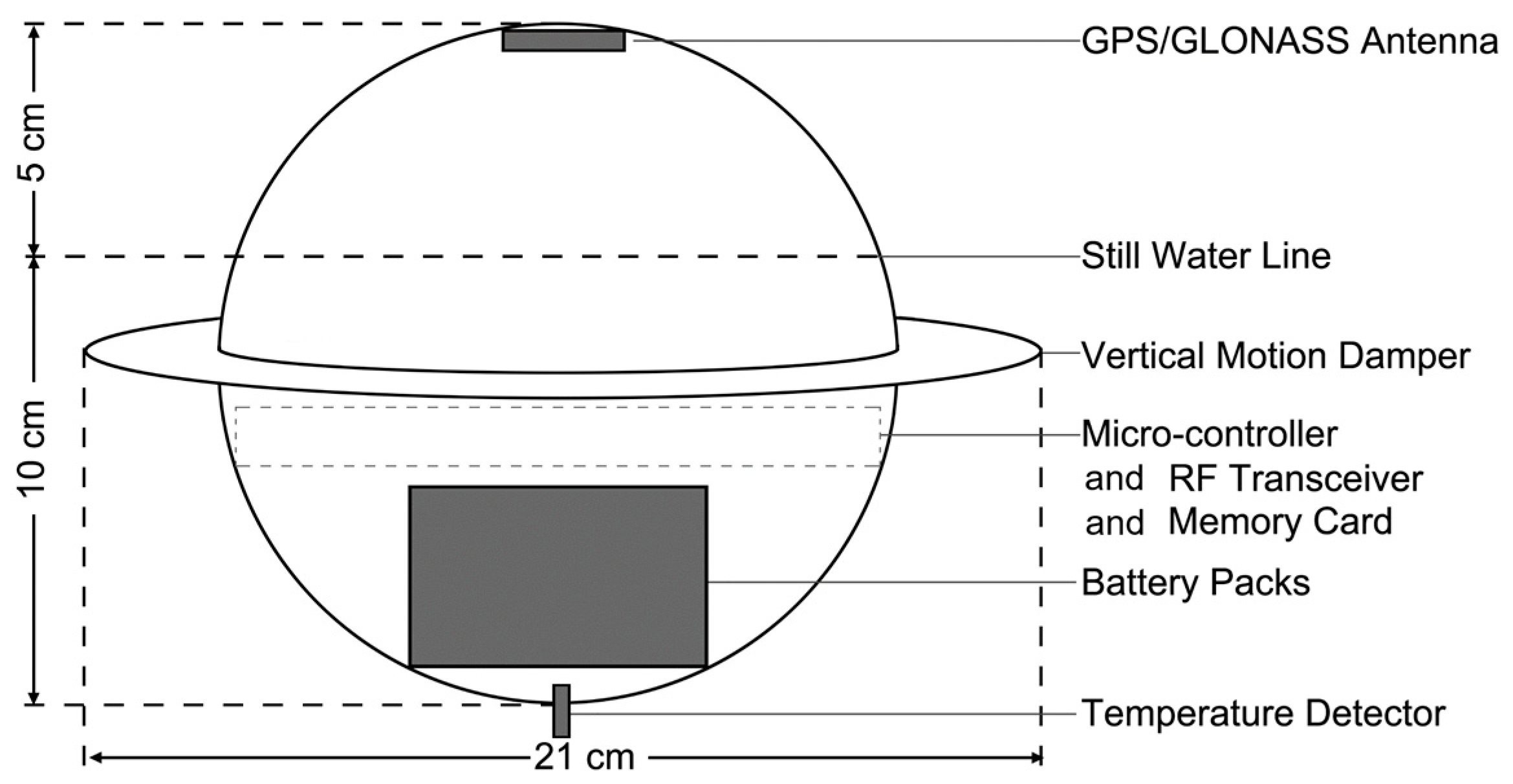
2.2.2. Sea Surface Temperature Measured by Drifter Array

Drifters equipped with temperature sensors were used to track the temperature changes of the warm water plume after its discharge into the sea. The structure of the sea surface drifter is shown in Figure 2. The drifter was a 15 cm diameter sphere, composed of an upper and lower hemisphere. A ring structure, like Saturn’s, was situated between the hemispheres to enhance the drifter’s resistance to tilting in water, thereby reducing the likelihood that the bottom-mounted thermometer would be exposed to air due to the drifter’s rolling motion. The satellite positioning antenna was positioned at the top of the upper hemisphere, with both GPS and GLONASS satellite positioning systems being utilized. The lower hemisphere, from top to bottom, housed the microprocessor, radio communicator, memory card, battery, and thermometer. The drifter maintained a height of approximately 5 cm above the sea surface to facilitate radio communication and satellite positioning. The drifter’s sampling frequency was 1 Hz, with raw data being recorded on an integrated SD card. Additionally, every 10 s, one in ten recorded readings was transmitted back to the coastal receiving station via radio communication, allowing for partial data backup.

In this study, the self-developed drifters were used to observe the mixing efficiency in the Lagrangian perspective. Mixing efficiency was reflected by the dispersion rate of the drifter array under the influence of multiple hydrodynamic processes. This mixing efficiency is called shear dispersion coefficient, k. The calculation formula is as follows [14,15]:

$$k={\displaystyle \frac{1}{4}}{\displaystyle \frac{d}{dt}}{\sigma }_x{\sigma }_y$$

(1)

where

$${\sigma }_x^2={\displaystyle \frac{1}{N-1}}{\displaystyle \sum _{i=1}^N}{\left[x_i-\overline{x}\right]}^2$$

(2)

$${\sigma }_y^2={\displaystyle \frac{1}{N-1}}{\displaystyle \sum _{i=1}^N}{\left[y_i-\overline{y}\right]}^2$$

(3)

where x and y are the east–west coordinates and north–south coordinates of the drifter, respectively. Subscript i denotes the ith drifter, and $\overline{x}$ and $\overline{y}$ are the center coordinates of the drifter array.

2.2.3. Nutrient Concentration Measurement of Water Samples

The sampling sites coincided with those of the CTD measurements conducted in the Danshui Estuary. At each site, seawater was collected at depths of 0, 3, 10, 25, 50, and 75 m. For stations with shallower water depths, the number of water layers sampled was adjusted accordingly. Therefore, the working time at each site ranged from 30 to 60 min, with a total accumulated station working time of about 400 min. To facilitate on-board operations, the working time was scheduled during the daytime. Water sampling began around 6:00 a.m. for both cruises, and all sampling operations were completed before sunset, around 18:00 p.m. The parameters assessed in the sampled water included dissolved oxygen concentration, chlorophyll concentration, and DIN concentration. These measurements were conducted only in the Danshui Estuary.

3. Results and Analysis

3.1. Analysis of the Stratification Phenomenon in Danshui Estuary

Stratification in the estuary is a critical factor influencing the mixing and diffusion of substances. The degree of stratification can be readily discerned from the thermohaline structure. Figure 3 presents the temperature and salinity profiles of the Danshui Estuary, with the horizontal axis representing the distance from the station to the estuary mouth. The CTD data in this figure were measured at the stations indicated by asterisks with red circles in Figure 1b. The data from the October 2016 cruise reveal that the water temperature and salinity are more uniform in the horizontal direction but exhibit significant variation in the vertical direction. Specifically, the surface layer is characterized by high temperature and low salinity, and the bottom layer by low temperature and high salinity, indicating pronounced stratification. In contrast, the data from the March 2017 cruise show a more uniform vertical distribution but horizontal variation, demonstrating significant vertical mixing.

Significant variations in chlorophyll and dissolved oxygen concentrations were observed between the two cruises under contrasting stratification conditions. During the October 2016 cruise, stratification was pronounced, hindering the transport of surface nutrients to deeper waters. Nutrients, primarily derived from river runoff, were concentrated at the sea surface, leading to a localized distribution of chlorophyll at the surface and a relatively high concentration of dissolved oxygen only in the upper water layers (Figure 4a,b). In contrast, during the March 2017 cruise, good vertical mixing in the estuary resulted in a uniform distribution of chlorophyll throughout the euphotic zone, which extends approximately 20 m below the surface in the coastal area (Figure 4c). Benefiting from the good vertical mixing, the chlorophyll concentration below the euphotic zone was significantly higher than that during the stratified conditions of the October 2016 cruise. It even reached a concentration level comparable to those at the surface during the October 2016 cruise. Regarding dissolved oxygen concentrations, the vertical mixing during the March 2017 cruise led to near-saturation levels throughout the water column (Figure 4d), which was nearly 30 percentage points higher than that during the stratified conditions of the October 2016 cruise.

The average water temperature during the October 2016 cruise ranged from approximately 25.8 to 27.3 °C, while it was 20.3 to 21.7 °C for the March 2017 cruise. The latter corresponds precisely to the suitable temperature for the growth and reproduction of the dominant estuarine phytoplankton species, Cyclotella, in the Danshui Estuary [16]. Furthermore, increased rainfall in spring (March 2017 cruise) compared to autumn (October 2016 cruise) leads to higher concentrations of nutrients delivered by runoff, promoting a period of vigorous phytoplankton growth. Vertical mixing further contributes to the high chlorophyll concentrations and near-saturation levels of dissolved oxygen observed in the spring estuary.

In short, estuarine stratification hinders the downward transfer of nutrients and dissolved oxygen, and subsequently alters the nitrogen cycle within the estuary. This is likely to exacerbate the decline in primary productivity and lead to other ecological problems.

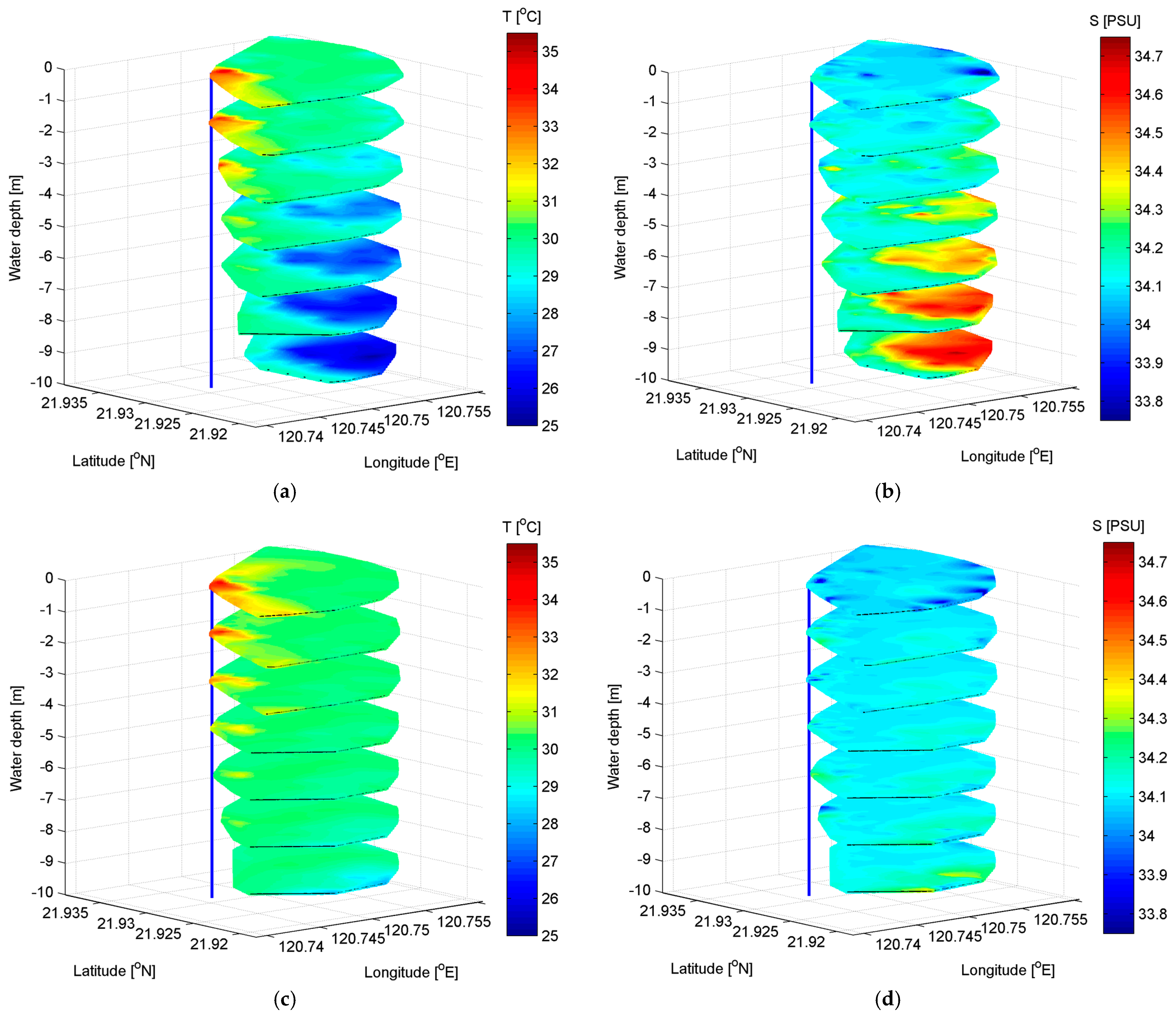
3.2. Upwelling of Cold Water Around the Thermal Discharge Outlet

This study also conducted a thermohaline structure survey in the thermal discharge area on 20 April 2017, similar to that in the Danshui Estuary. However, due to the smaller spatial scale and more rapid changes in the hydrodynamics of the thermal discharge, an underway CTD (UCTD) with a 16 Hz sampling frequency was employed for rapid, continuous observations during flood and ebb tides. Figure 5 displays the 3D thermohaline structure of the flood and ebb tides in the thermal discharge area. It is evident that the area of the locally high-temperature water mass, resulting from the thermal discharge, diminishes significantly with depth, reaching 4.5 to 6.0 m underwater regardless of the tide state (Figure 5a,c). Jan et al. [13] also identified this 5 to 7 m-thick thermal plume immediately outside the outlet. Figure 5 further reveals a phenomenon unique to the flood tide: a low-temperature, high-salinity water mass rises from the bottom to a depth of approximately 6 m. The maximum temperature difference between the surface and the bottom is about 9 °C, and the maximum salinity difference is around 1.0 PSU. The area of the low-temperature, high-salinity water mass (25 °C, 34.7 PSU) from the seabed gradually decreases with decreasing water depth. Jan and Chen [17] suggested that deep-sea internal waves from the Bashi Channel break up under the influence of the Hengchun ridge, and the corresponding low-temperature, high-salinity water mass is transported to the outlet by tidal currents.

Due to the upwelling of cold and salty water during the flood tide and the continuous thermal discharge on the sea surface, the stratification intensity in the thermal discharge area was expected to exhibit significant differences between the flood and ebb tides. Based on the temperature and salinity data collected by the UCTD, along with the velocity profiles measured by an upward-looking ADCP (Acoustic Doppler Current Profiler, Workhorse II Sentinel 600, Teledyne RD Instruments Co., Ltd., Poway, CA, USA. Mounted at the red triangle in Figure 1c), Richardson numbers were calculated. During the flood tide, the maximum Richardson number reached approximately 0.7 ± 0.07, significantly higher than the critical value of 0.25. In contrast, the Richardson number remained below 0.1 ± 0.06 during the ebb tide. This indicates that stratification during the flood tide is strong, greatly limiting the vertical exchange of water.

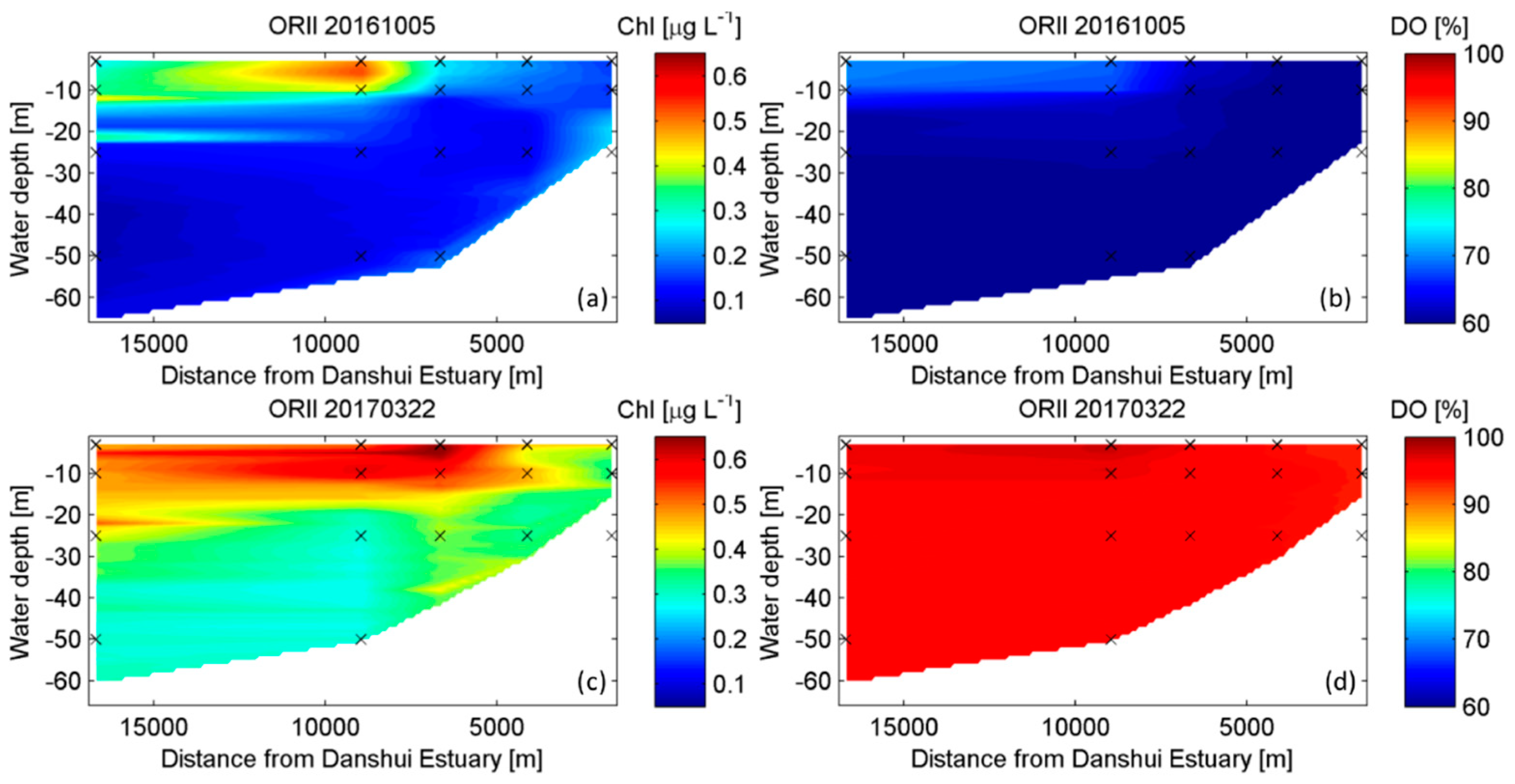
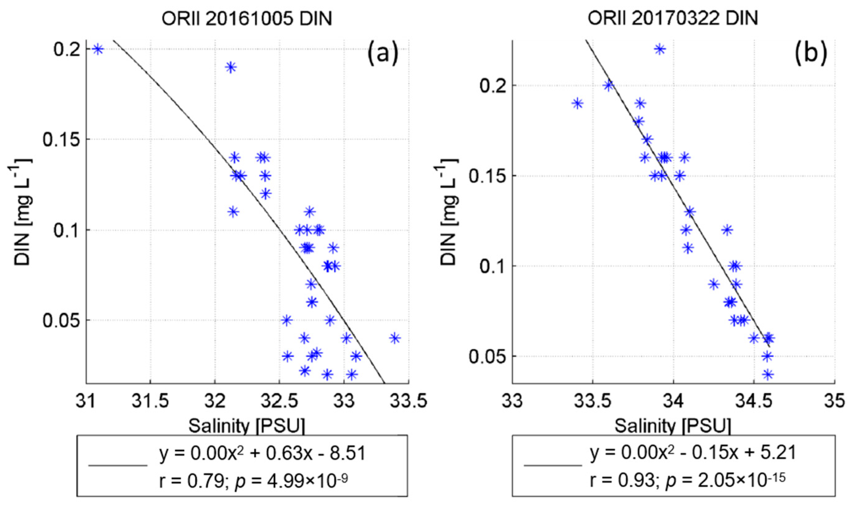
3.3. The Mixing Process of Nutrients in the Danshui Estuary

Nutrient transport in estuaries is mainly influenced by the mixing of freshwater and saltwater, leading to relatively conservative diffusive dilution [18]. In waters with high productivity, absorption by organisms often results in a non-conservative distribution of nutrients [19,20]. Additionally, the adsorption/desorption of suspended particles and chemical processes can also cause changes in nutrient concentrations. As freshwater from the estuary expands into the sea, nutrient concentrations form a gradient under the influence of complex estuarine processes. Salinity is considered an excellent conservative tracer in the ocean because it is not created or consumed by chemical or biological processes.

This study employed the theoretical conservative mixing line to analyze the dispersion behavior of DIN in the estuarine waters. Figure 6 illustrates the relationship between DIN concentration and salinity in the Danshui Estuary. Wu et al. [21] proposed four hypothetical scenarios to show the trend of DIN vs. salinity from freshwater to full seawater. They concluded that if DIN vs. salinity forms a straight line, DIN is considered to act conservatively. The non-linear DIN vs. salinity relationships can be attributed to biological and chemical activities and mixing between riverine water and seawater. Therefore, this study uses non-linear equations to fit the relationship between DIN concentration and salinity. If the fitting results show that the coefficient of the non-linear term is zero or nearly zero, it indicates that DIN exhibits conservative behavior. Conversely, it suggests that DIN is removed from (or added to) the system by processes such as phytoplankton growth, sedimentation, denitrification, and so on (additional discharges, sediment recycling, etc.). The fitted equations are displayed below the panels of Figure 6. During the October 2016 cruise, y = 0.00x² + 0.63x − 8.51 (r = 0.79, p < 0.01), where y represents DIN and x represents salinity. During the March 2017 cruise, y = 0.00x² − 0.15x + 5.21 (r = 0.93, p < 0.01). Both non-linear term coefficients are almost 0.00, indicating that the change in DIN concentration is strongly associated with physical mixing processes across the Danshui Estuary in both cruises. In other words, although vertical mixing is suppressed during significant stratification, the variation of nutrient concentration with salinity is similar to that during non-stratified conditions. Therefore, we believe that horizontal mixing is the primary process in the Danshui Estuary, which will be discussed in detail in Section 3.5.

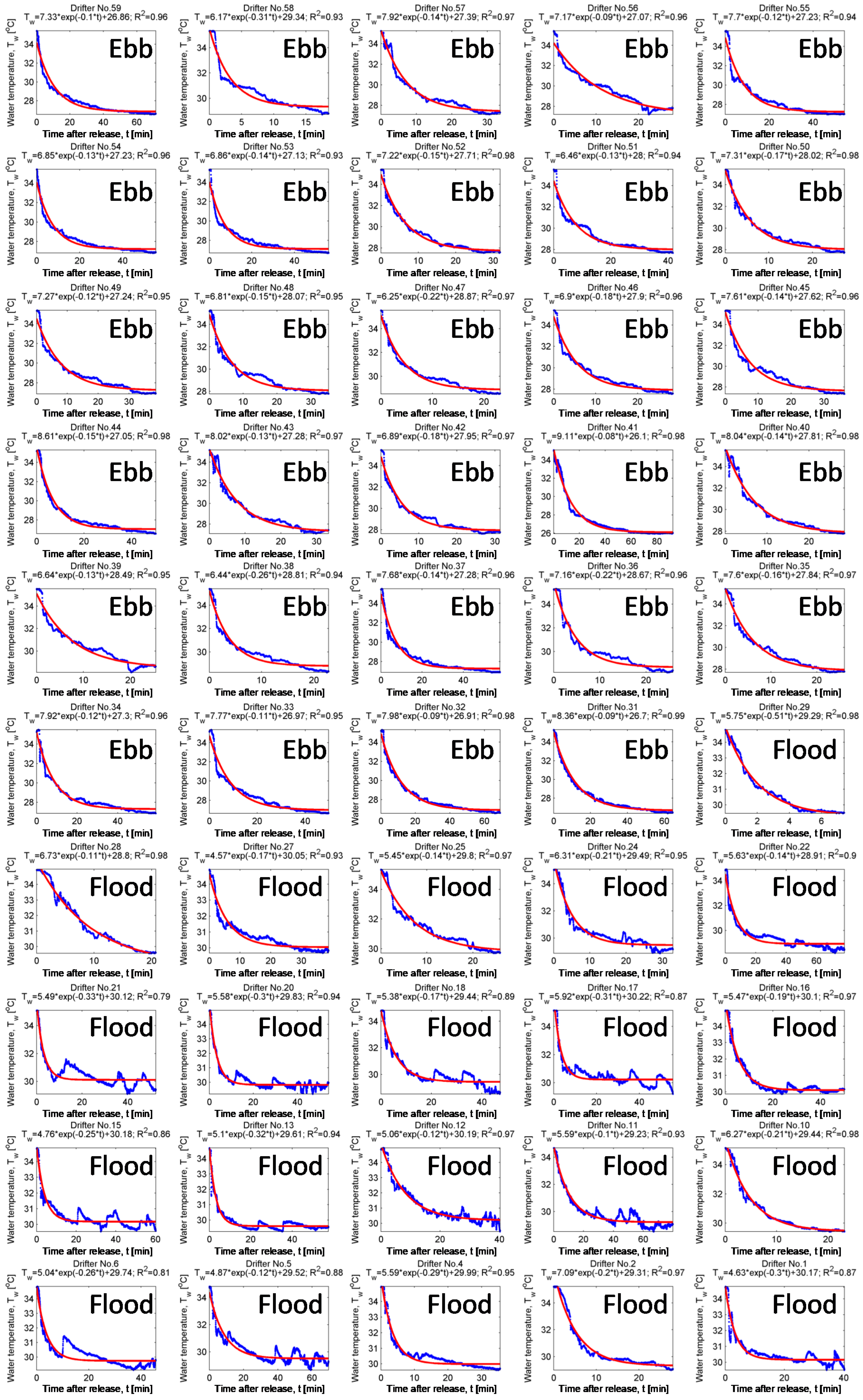
3.4. Attenuation Curve of Water Temperature in Thermal Discharge Area

The thermal discharge from a nuclear power plant introduces heat into coastal waters, which is primarily dissipated through two mechanisms. First, heat is lost to the atmosphere across the air–sea interface via sensible and latent heat fluxes. Second, heat is exchanged through mixing with the surrounding seawater. The former is influenced by air temperature, water temperature, wind speed, and air humidity, while the latter is predominantly determined by the intensity of mixing. Based on the observed meteorological data (indicated by the red pentagram in Figure 1c, Weather Transmitter, Model: WXT520, Vaisala Co., Ltd., Vantaa, Finland), the sensible and latent heat fluxes during the observation period were estimated to be −0.028 to −0.022 W m⁻² and 0.051 to 0.274 W m⁻², respectively. A positive flux indicates heat transfer from the sea to the air, while a negative flux suggests the opposite direction. Consequently, the air–sea heat flux was found to be negligible, and the reduction in water temperature was primarily attributed to the physical mixing process of the water.

Water temperature is a parameter that is easily monitored in real-time. Water temperature is also an excellent conservative tracer as it is minimally affected by chemical or biological processes. As a tracer for thermal pollution, it is particularly suitable for quantitative analysis of the mixing characteristics of waters at thermal discharge outlets. Drifter clusters were used to track the temperature changes of the warm water after it entered the sea. A temperature decay curve was further employed to calculate the e-folding scale of water temperature. Regression analysis was performed, with time (t, in minutes) as the independent variable and sea surface temperature (T_W, in °C) as the dependent variable. The reciprocal of the power coefficient was referred to the e-folding scale [21]. If the independent variable is time, the e-folding scale indicates the time required for water temperature to decay from its initial value to 1/e of that value. If the independent variable is distance, the e-folding scale represents the extent of the near-field mixing zone, where mixing is the most intense and dilution is the most rapid [21]. Figure 7 shows the fitting results of the water temperature attenuation curve. The blue points represent water temperatures measured by sea surface drifters, and the red solid lines are the fitting curves, with R² values ranging from 0.95 to 0.99. The fitting results of each drifter are summarized in

Table 1. Coefficients of water temperature fitting curves around the thermal discharge area.

No.$	a #	b #	c #	R2	e-Folding Scale [min]	Tide	No. $	a	b #	c #	R2	e-Folding Scale [min]	Tide
4	1.72	−0.4955	30.41	0.96	2.02	Ebb	3	2.26	−0.1472	29.20	0.95	6.79	Flood
12	3.30	−0.6083	31.10	0.97	1.64	Ebb	9	2.33	−0.1854	31.94	0.98	5.39	Flood
15	1.57	−0.4654	31.14	0.95	2.15	Ebb	21	2.66	−0.2935	31.79	0.97	3.41	Flood
36	3.48	−0.4586	30.94	0.97	2.18	Ebb	24	2.36	−0.3370	31.96	0.96	2.97	Flood
37	1.45	−0.4645	31.58	0.97	2.15	Ebb	13	2.95	−0.2884	30.97	0.99	3.47	Flood
38	2.32	−0.4932	31.30	0.97	2.03	Ebb	20	2.67	−0.3902	31.51	0.97	2.56	Flood
39	1.24	−0.4893	30.65	0.98	2.04	Ebb	22	3.38	−0.1223	29.69	0.98	8.18	Flood
40	0.99	−0.3082	31.28	0.95	3.24	Ebb	25	2.58	−0.3904	31.79	0.97	2.56	Flood
47	3.24	−0.4204	31.19	0.98	2.38	Ebb
48	1.31	−0.4695	31.56	0.95	2.13	Ebb
49	1.64	−0.4851	31.93	0.98	2.06	Ebb
51	1.70	−0.4187	31.15	0.98	2.39	Ebb
52	1.47	−0.6863	31.82	0.98	1.46	Ebb

^$: ID of drifter. ^#: Tw = ae^bt + c.

. The average e-folding times during the ebb tide and flood tide are 2.14 ± 0.40 min and 4.19 ± 2.33 min, respectively. The temperature decay rate during the ebb tide is nearly twice that of the flood tide.

Previous estimates of the air–sea heat flux revealed it to be negligible. Furthermore, the Richardson number indicated significant stratification, which suppresses vertical mixing efficiency strongly during the flood tide. In Section 3.5, we will provide a detailed estimation of horizontal mixing efficiency during flood and ebb tides, ultimately clarifying the reasons behind the slower temperature decline observed during the flood tide.

3.5. The Horizontal Dispersion Coefficient Measured Using Sea Surface Drifter Array

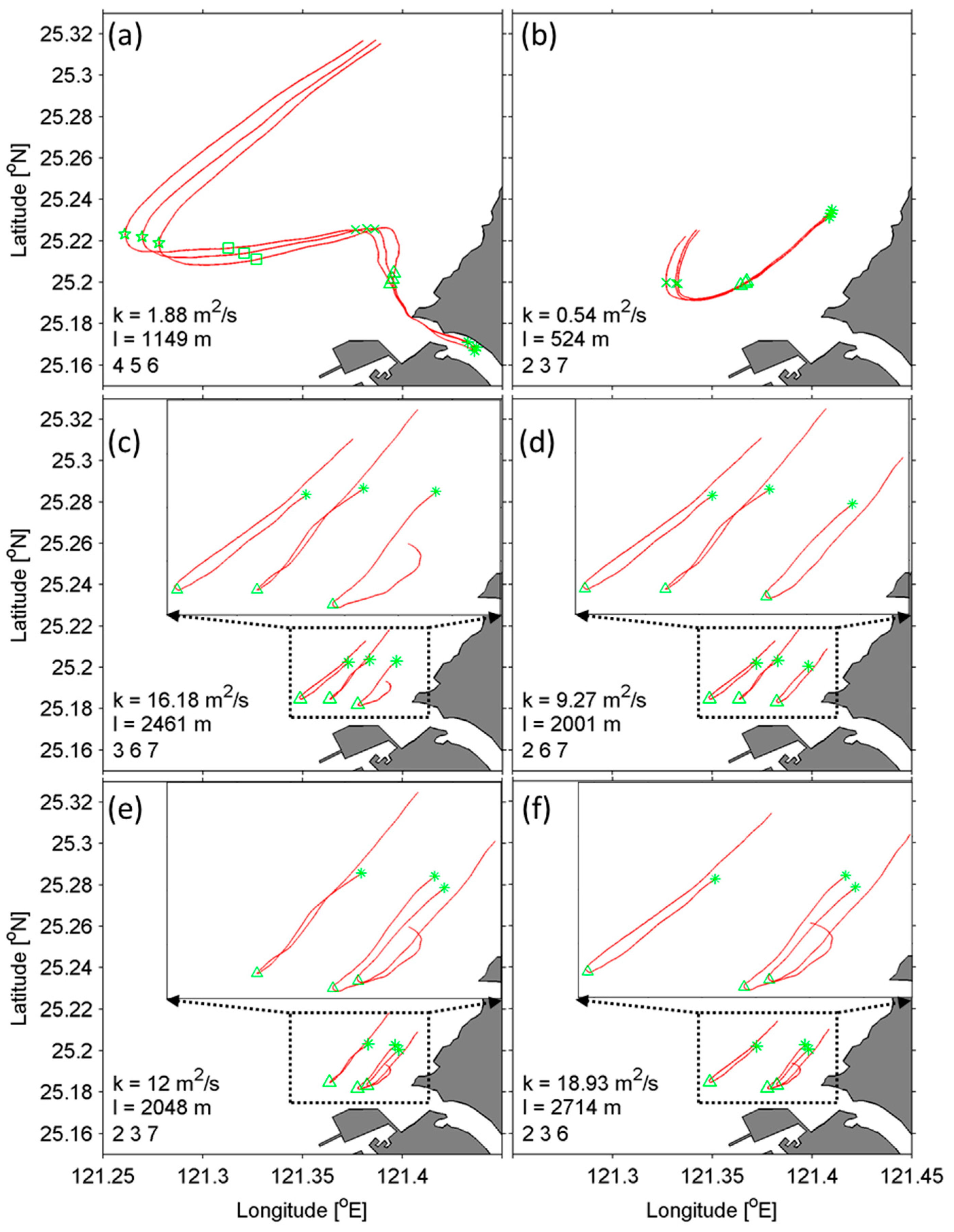
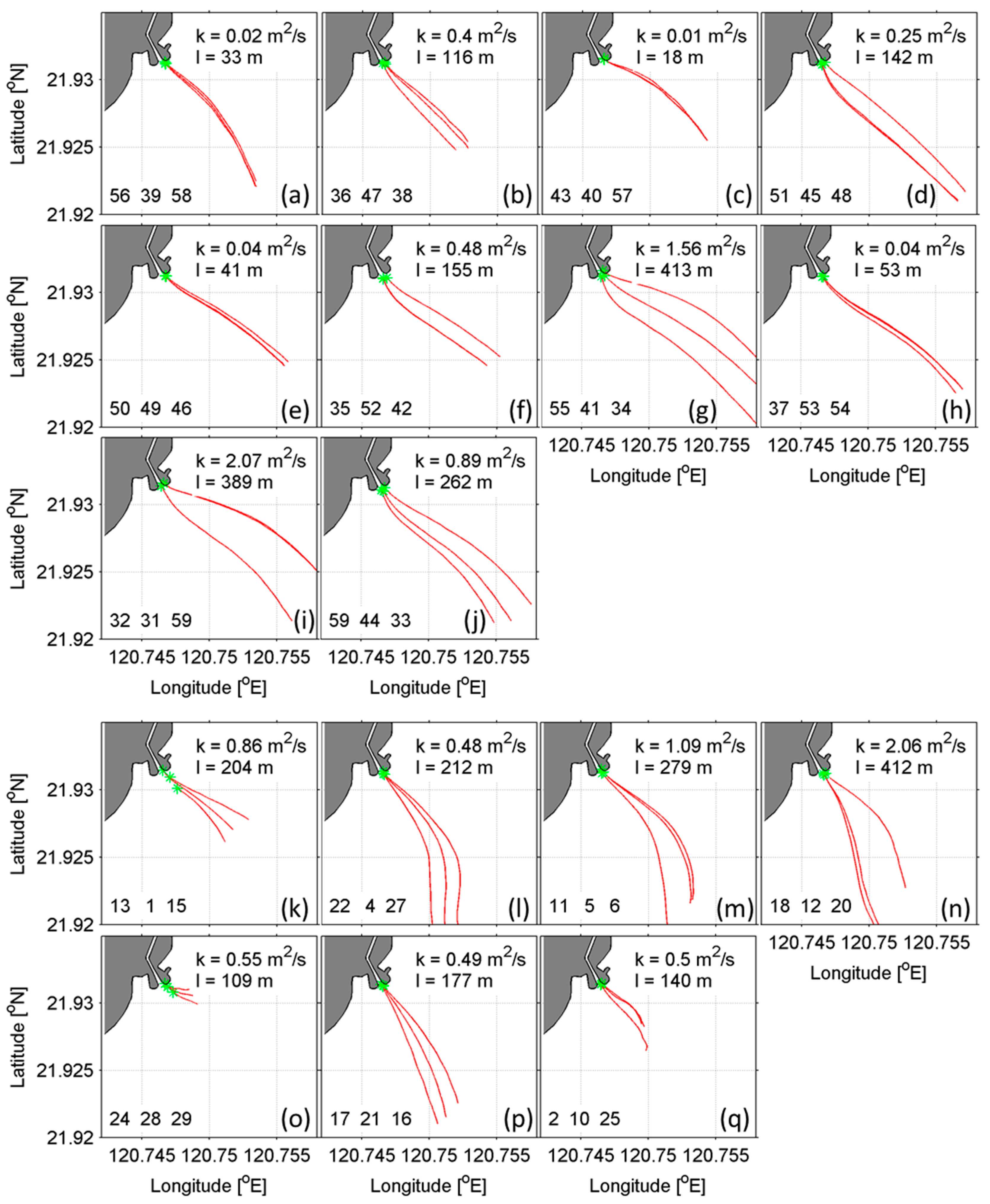
3.5.1. Dispersion Coefficient of Danshui Estuary and Thermal Discharge Area

The previous analysis suggests that the relationship between DIN concentration and salinity during the two cruises generally aligns with the theoretical dilution curves, indicating that mixing in the Danshui Estuary is primarily driven by physical processes. Notably, during the October 2016 cruise, when stratification was pronounced and vertical mixing was suppressed, DIN concentrations still indicated that physical mixing was predominant. Consequently, this study infers that horizontal mixing dominates in the Danshui Estuary. Figure 8 shows the horizontal dispersion coefficients of the Danshui Estuary based on the sea surface drifter array. Figure 8a,b presents the results under strong stratification conditions (October 2016 cruise), while Figure 8c–f shows the results when the water is well-mixed vertically (March 2017 cruise). The red solid lines in Figure 8 represent the trajectories of the drifters, and the asterisks (*) indicate the release points. The symbols △, ×, □, and ☆ along the trajectories denote the positions of the drifters at 10,000, 20,000, 30,000, and 40,000 s after release, respectively. The lower left corner of each panel provides the dispersion coefficient (without spatial scale calibration) calculated by Equation (1), the spatial scale calculated by Equation (5), and the IDs of the three drifters. The results reveal that the average dispersion coefficient in the Danshui Estuary under strong stratification effects is 9.16 ± 1.57 m² s⁻¹ (spatial scale calibrated), while under well-mixed vertical conditions, the average dispersion coefficient is 11.84 ± 1.71 m² s⁻¹ (spatial scale calibrated). Although there is no significant difference between the two (p > 0.05), both values are several times greater than the horizontal dispersion coefficient obtained by Tseng [14] in the Tseng-wen Estuary, southwestern Taiwan, using the same observational methods, which ranged from 1.52 to 5.53 m² s⁻¹ (spatial scale calibrated). Therefore, we can see that the intensity of horizontal mixing in the Danshui Estuary is significant.

The annual DIN export from the Danshui River is approximately 8020 kg N km⁻² year⁻¹ [9], which is significantly higher than that of the Pearl River Estuary, estimated at 602–1148 kg N km⁻² year⁻¹ [22,23]. The Pearl River Estuary ranks as the fourth most polluted estuary globally [24], whereas the Danshui Estuary is not included in the list of 31 estuaries. Based on the drifter trajectories data published by Gu et al. [25], we calculated the spatial scale calibrated dispersion coefficient for the Pearl River Estuary. It was approximately 1.79 m² s⁻¹ by assuming that the dispersion coefficient and spatial scale in the Pearl River Estuary conform to Richardson’s 4/3 law. Horizontal mixing is a significant contributor to estuarine mixing, and the severe pollution in the Pearl River Estuary may be attributed to its low horizontal mixing efficiency. In contrast, the high DIN concentrations in the Danshui Estuary, coupled with few pollution incidents, are likely due to its high horizontal mixing efficiency. This observation is further supported by the findings of Wang et al. [26], who used the HEM-2D model to evaluate the water residence time in the Danshui River, finding it to be only one to two days. Such a short residence time implies that even with high nutrient concentrations, phytoplankton cannot grow in large numbers in the water, resulting in fewer pollution incidents in the Danshui Estuary.

The analysis in Section 3.4 highlights the necessity for a comprehensive estimation of horizontal mixing efficiency during flood and ebb tides to elucidate the reasons behind the slower temperature decline during the flood tide. This study employs observational data from a drifter array to estimate this mixing efficiency. Figure 9 presents the dispersion coefficients at the thermal discharge outlet during the flood and ebb tide. Figure 9a–j displays the results for the ebb-tide period, while Figure 9k–q shows the results for the flood-tide period. After spatial scale calibration, the average dispersion coefficient during the flood tide was found to be 0.53 ± 0.18 m² s⁻¹, and for ebb tides it averaged 0.46 ± 0.17 m² s⁻¹, with no significant difference between the two tide periods (p > 0.05). Consequently, this study concludes that the slower temperature decline during the flood tide is likely attributed to the strong stratification present at that time.

3.5.2. Relationship Between Horizontal Dispersion and the Drifter Array’s Spatial Scale

Compared to the Danshui Estuary, the spatial scale of the drifter array at the thermal discharge outlet was considerably smaller, and its horizontal dispersion coefficient was an order of magnitude lower. Suara et al. [27] conducted experiments in Eprapah Creek using drifters and obtained lateral/streamwise dispersion coefficients ranging from 0.05 to 0.57 m² s⁻¹. Suara, Brown, and Borgas [28] estimated the shear dispersion coefficient within a tidal shallow estuary with drifters and found that the coefficient varied between 0.001 and 0.02 m² s⁻¹. In their observational experiments, the spatial scale of the drifter arrays was also relatively small. In other words, the values of the horizontal dispersion coefficient observed with drifter arrays are significantly related to their spatial scale. The dispersion of the drifter cluster is primarily caused by eddies that are comparable in size to, or smaller than, their distribution range. If the distribution area of the drifter array is small, only small-scale eddies contribute to the dispersion; if the distribution area is large, larger-scale eddies together with small-scale eddies will influence the dispersion of the drifter cluster. The theoretical relationship between the dispersion coefficient and spatial scale should conform to Richardson’s 4/3 law:

$$k=\alpha l^{4/3}$$

(4)

where, α is a parameter related to energy dissipation with theoretical ranges of 0.000090~0.003250 m^2/3 s⁻¹ [29]. The calculation formula of spatial scale is as follows:

$$l=3\sqrt{D}$$

(5)

where $D=2{\sigma }_x{\sigma }_y$.

Figure 10 illustrates the relationship between the dispersion coefficient observed from the drifter array and the spatial scale of the arrays, showing a high degree of correlation coefficient. The α values for the Danshui Estuary and the thermal discharge outlet are 0.000467 m^2/3 s⁻¹ (r = 0.96, p < 0.01) and 0.000609 m^2/3 s⁻¹ (r = 0.96, p < 0.01), respectively. All of these values fall within the acceptable limits proposed by Monin and Yaglom [29]. The relationship between the dispersion coefficients and spatial scales derived from this study and previous research [30,31,32,33] are listed in

Table 2. Comparison of relationships between k and l derived from this study and previous studies.

No.	k vs. l	Sources
1	k = 0.000455l4/3	Danshui Estuary (This study)
2	k = 0.000609l4/3	Thermal discharge outlet (This study)
3	k = 0.000206l1.15	Okubo [30]
4	k = 0.000123l1.22	Yanagi et al. [31]
5	k = 0.000004l1.92	Michida et al. [32]
6	k = 0.000147l4/3	Matsuzaki and Fujita [33]

.

By examining the exponent parts, previous studies either conform to or closely approximate Richardson’s 4/3 law. The most different one is the work of Michida et al. [32], where the indices of 1.92 notably exceeds the value of 4/3, and the corresponding α value falls outside the theoretical range; thus, it is excluded from further discussion. Regarding the α values, all are found to be within the theoretical bounds. Under the same spatial scale, a larger α value corresponds to a larger dispersion coefficient (k). From a purely numerical perspective, when the spatial scales are equal, the horizontal dispersion coefficient at the thermal discharge outlet is 1.34 times that of the Danshui Estuary. However, the spatial scale range of the drifter array in the Danshui Estuary was approximately 500–3000 m, while that at the thermal discharge outlet was about 20–400 m, with no overlapping areas. Such extrapolation is not rigorous and necessitates further experimental validation.

4. Conclusions

This study provides an investigation into the mixing and diffusion characteristics of the Danshui Estuary and a thermal discharge outlet of a power plant, revealing the mixing properties of the estuarine environments under varying dynamic conditions and their dominant factors. In the Danshui Estuary, significant stratification during the October 2016 cruise suppressed vertical mixing, yet the nutrient concentration varied with salinity in accordance with the theoretical dilution curve, indicating that horizontal mixing is the dominant process. Observations from the drifter array revealed horizontal dispersion coefficients of 9.16 ± 1.57 m² s⁻¹ and 11.84 ± 1.71 m² s⁻¹ for the two cruises in the Danshui Estuary. Both of them are significantly higher than those of the Tseng-wen Estuary [14] and the Pearl River Estuary [25]. This further explains why the DIN concentrations in the Danshui Estuary are much higher than the global average, yet estuarine pollution incidents are rare.

For the thermal discharge outlet of the power plant, the upwelling of cold and high-salinity water during the flood tide (which disappears during ebb tides) significantly impacts the mixing characteristics of the discharge area. Observations from drifter arrays showed horizontal dispersion coefficients of 0.53 ± 0.18 m² s⁻¹ during the flood tide and 0.46 ± 0.17 m² s⁻¹ during the ebb tide, indicating nearly identical horizontal mixing intensities between flood and ebb tides. However, the rate of temperature decline during the ebb tide is nearly twice that of the flood tide. Analysis of 3D thermohaline structure data and ADCP data revealed that the Richardson number during the flood tide reached 0.7 ± 0.07. This finding suggests that the stratification effect is likely the cause of the slower temperature decline during the flood tide. Therefore, it is recommended that the power plant increases discharge during the ebb tide and decreases it during the flood tide to minimize the impact of waste heat on the marine environment. Due to the fixed nature of a thermal discharge outlet and its presence throughout the entire lifecycle of a nuclear power plant, the environmental impact of waste heat accumulates over time, making its long-term impacts more significant. This study only observed the patterns on the tidal timescale, and there is no data to support a long-term impacts analysis. Future research could consider incorporating satellite remote sensing data for a comprehensive assessment and to develop effective long-term management strategies.

Additionally, the observations from drifter arrays at both the Danshui Estuary and the thermal discharge outlet conform to Richardson’s 4/3 law. Although extrapolated results indicate that the horizontal dispersion coefficient at the thermal discharge outlet is 1.34 times that of the Danshui Estuary, further experimental validation is needed due to the lack of overlapping spatial scale ranges between the two.

In summary, this study not only clarifies the mixing characteristics of the Danshui Estuary and the thermal discharge outlet under different dynamic conditions, but also provides a scientific basis for the environmental management of the power plant’s thermal discharge. Future research could explore how mixing dynamics affect the transport of substances and environmental responses, thereby promoting sustainable management and protection of estuarine environments.

References

1. Grasso, F.; Caillaud, M. A ten-year numerical hindcast of hydrodynamics and sediment dynamics in the Loire Estuary. Sci. Data 2023, 10, 394. [Google Scholar] [CrossRef] [PubMed]
2. Dzwonkowski, B.; Kang, X.; Sahoo, B.; Veeramony, J.; Mitchell, S.; Xia, M. Mixing and transport in estuaries and coastal waters a special issue in Estuarine Coastal and Shelf Science. Estuar. Coast. Shelf Sci. 2023, 288, 108370. [Google Scholar] [CrossRef]
3. Boyer, E.W.; Howarth, R.W. Nitrogen fluxes from rivers to the coastal oceans. In Nitrogen in the Marine Environment; Elsevier Inc.: Amsterdam, The Netherlands, 2008; pp. 1565–1587. [Google Scholar]
4. Vitousek, P.M.; Menge, D.N.; Reed, S.C.; Cleveland, C.C. Biological nitrogen fixation: Rates, patterns and ecological controls in terrestrial ecosystems. Philos. Trans. R. Soc. B Biol. Sci. 2013, 368, 20130119. [Google Scholar] [CrossRef] [PubMed]
5. Liu, K.-K.; Yan, W.J.; Lee, H.-J.; Chao, S.-Y.; Gong, G.-C.; Yeh, T.-Y. Impacts of increasing dissolved inorganic nitrogen discharged from Changjiang on primary production and seafloor oxygen demand in the East China Sea from 1970 to 2002. J. Mar. Syst. 2015, 141, 200–217. [Google Scholar] [CrossRef]
6. Glavovic, B.; Limburg, K.; Liu, K.-K.; Emeis, K.-C.; Thomas, H.; Kremer, H.; Avril, B.; Zhang, J.; Mulholland, M.R.; Glaser, M.; et al. Living on the Margin in the Anthropocene: Engagement arenas for sustainability research and action at the ocean–land interface. Curr. Opin. Environ. Sustain. 2015, 14, 232–238. [Google Scholar] [CrossRef]
7. Diaz, R.J.; Rosenberg, R. Spreading Dead Zones and Consequences for Marine Ecosystems. Science 2008, 321, 926–929. [Google Scholar] [CrossRef]
8. Dumont, E.; Harrison, J.A.; Kroeze, C.; Bakker, E.J.; Seitzinger, S.P. Global distribution and sources of dissolved inorganic nitrogen export to the coastal zone: Results from a spatially explicit, global model. Glob. Biogeochem. Cycles 2005, 19, 4. [Google Scholar] [CrossRef]
9. Huang, J.-C.; Lee, T.-Y.; Lin, T.-C.; Hein, T.; Lee, L.-C.; Shih, Y.-T.; Kao, S.-J.; Shiah, F.-K.; Lin, N.-H. Effects of different N sources on riverine DIN export and retention in a subtropical high-standing island, Taiwan. Biogeosciences 2016, 13, 1787–1800. [Google Scholar] [CrossRef]
10. Rahman, W.; Abedin, M.Z.; Chowdhury, S. Efficiency analysis of nuclear power plants: A comprehensive review. World J. Adv. Res. Rev. 2023, 19, 527–540. [Google Scholar] [CrossRef]
11. Huang, J.-C.; Lin, C.-C.; Chan, S.-C.; Lee, T.-Y.; Hsu, S.-C.; Lee, C.-T.; Lin, J.-C. Stream discharge characteristics through urbanization gradient in Danshui River, Taiwan: Perspectives from observation and simulation. Environ. Monit. Assess. 2012, 184, 5689–5703. [Google Scholar] [CrossRef] [PubMed]
12. Lee, T.-Y.; Shih, Y.-T.; Huang, J.-C.; Kao, S.-J.; Shiah, F.-K.; Liu, K.-K. Speciation and dynamics of dissolved inorganic nitrogen export in the Danshui River, Taiwan. Biogeosciences 2014, 11, 5307–5321. [Google Scholar] [CrossRef]
13. Jan, S.; Chen, C.-T.A.; Tu, Y.-Y.; Tsai, H.-S. Physical Properties of Thermal Plumes from a Nuclear Power Plant in the Southernmost Taiwan. J. Mar. Sci. Technol. 2004, 12, 10. [Google Scholar] [CrossRef]
14. Tseng, R.-S. On the Dispersion and Diffusion Near Estuaries and Around Islands. Estuar. Coast. Shelf Sci. 2002, 54, 89–100. [Google Scholar] [CrossRef]
15. Manning, J.; Churchill, J. Estimates of dispersion from clustered-drifter deployments on the southern flank of Georges Bank. Deep. Sea Res. Part II Top. Stud. Oceanogr. 2006, 53, 2501–2519. [Google Scholar] [CrossRef]
16. Chen, Y.-L.; Hsieh, C.-H. Seasonal variations in phytoplankton community structure in the Danshui River estuary, Taiwan. J. Mar. Syst. 2012, 98, 1–12. [Google Scholar]
17. Jan, S.; Chen, C.A. Potential biogeochemical effects from vigorous internal tides generated in Luzon Strait: A case study at the southernmost coast of Taiwan. J. Geophys. Res. Ocean. 2009, 114, 4. [Google Scholar] [CrossRef]
18. Gao, L.; Li, D.; Zhang, Y. Nutrients and particulate organic matter discharged by the Changjiang (Yangtze River): Seasonal variations and temporal trends. J. Geophys. Res. Biogeosci. 2012, 117, G04001. [Google Scholar] [CrossRef]
19. Raven, J.A.; Taylor, R. Macroalgal growth in nutrient-enriched estuaries: A biogeochemical and evolutionary perspective. Water Air Soil Pollut. Focus 2003, 3, 7–26. [Google Scholar] [CrossRef]
20. Mu, J.; Zhang, S.; Liang, C.; Xian, W.; Shen, Z. Temporal and spatial distribution and mixing behavior of nutrients in the Changjiang River Estuary. Mar. Sci. 2020, 44, 19–35. [Google Scholar]
21. Marmorino, G.; Savelyev, I.; Smith, G.B. Surface thermal structure in a shallow-water, vertical discharge from a coastal power plant. Environ. Fluid Mech. 2015, 15, 207–229. [Google Scholar] [CrossRef]
22. Liu, S.M.; Hong, G.-H.; Zhang, J.; Ye, X.W.; Jiang, X.L. Nutrient budgets for large Chinese estuaries. Biogeosciences 2009, 6, 2245–2263. [Google Scholar] [CrossRef]
23. Lu, F.-H.; Ni, H.-G.; Liu, F.; Zeng, E.Y. Occurrence of nutrients in riverine runoff of the Pearl River Delta, South China. J. Hydrol. 2009, 376, 107–115. [Google Scholar] [CrossRef]
24. Halpern, B.S.; Ebert, C.M.; Kappel, C.V.; Madin, E.M.; Micheli, F.; Perry, M.; Selkoe, K.A.; Walbridge, S. Global priority areas for incorporating land–sea connections in marine conservation. Conserv. Lett. 2009, 2, 189–196. [Google Scholar] [CrossRef]
25. Gu, J.; Zhang, Y.; Tuo, P.; Hu, Z.; Chen, S.; Hu, J. Surface floating objects moving from the Pearl River Estuary to Hainan Island: An observational and model study. J. Mar. Syst. 2024, 241, 103917. [Google Scholar] [CrossRef]
26. Wang, C.-F.; Hsu, M.-H.; Kuo, A.Y. Residence time of the Danshuei River estuary, Taiwan. Estuar. Coast. Shelf Sci. 2004, 60, 381–393. [Google Scholar] [CrossRef]
27. Suara, K.; Wang, C.; Feng, Y.; Brown, R.J.; Chanson, H.; Borgas, M. High-Resolution GNSS-Tracked Drifter for Studying Surface Dispersion in Shallow Water. J. Atmos. Ocean. Technol. 2015, 32, 579–590. [Google Scholar] [CrossRef]
28. Suara, K.; Brown, R.; Borgas, M. Eddy diffusivity: A single dispersion analysis of high resolution drifters in a tidal shallow estuary. Environ. Fluid Mech. 2016, 16, 923–943. [Google Scholar] [CrossRef]
29. Monin, A.S.; Yaglom, A.M. Statistical Fluid Mechanics: Mechanics of Turbulence; MIT Press: Cambridge, MA, USA, 1975; Volume 2, pp. 551–567. [Google Scholar]
30. Okubo, A. Oceanic diffusion diagrams. Deep. Sea Res. Oceanogr. Abstr. 1971, 18, 789–802. [Google Scholar] [CrossRef]
31. Yanagi, T.; Murashita, K.; Higuchi, H. Horizontal turbulent diffusivity in the sea. Deep Sea Res. Part A Oceanogr. Res. Pap. 1982, 29, 217–226. [Google Scholar] [CrossRef]
32. Michida, Y.; Tanaka, K.; Komatsu, T.; Ishigami, K.; Nakajima, M. Effects of divergence, convergence, and eddy diffusion upon the transport of objects drifting on the sea surface. Bull. Coast. Oceanogr. 2009, 46, 77–83. [Google Scholar]
33. Matsuzaki, Y.; Fujita, I. Horizontal Turbulent Diffusion at Sea Surface for Oil Transport Simulation. Coast. Eng. Proc. 2014, 1, 8. [Google Scholar] [CrossRef]
Figure 1. Study areas. There are two red boxes in (a). The box on the north side shows the location of the Danshui Estuary; details are shown in (b). The box on the south side shows the location of the thermal discharge area of the nuclear power plant; details are shown in (c). Asterisks (*) in (b) show the locations where the CTD measurements and water sample collections were conducted. The CTD data collected from the stations marked as asterisks with a red circle in (b) was further analyzed in Section 3.1. Dots (·) in (c) show the locations where the underway CTD measurements were conducted. A weather transmitter is installed at the point marked with the red pentagram. The red triangle (△) shows the location of an up-looking ADCP.
Jmse 12 02353 g001
Figure 2. Structure of self-developed sea surface drifter with a temperature detector at the bottom.
Jmse 12 02353 g002
Figure 3. Temperature and salinity profiles of Danshui Estuary. (a,c): temperature profiles. (b,d): salinity profiles. The CTD data for this figure were collected from the stations marked as asterisks with a red circle in Figure 1b. The horizontal axis represents the distance of each station from the estuary mouth. The x-markers on the graph indicate the actual sampling locations and their corresponding water depths. ORII represents Ocean Research Vessel No. 2, and 20161005 (20170322) means the date of 5 October 2016 (22 March 2017).
Jmse 12 02353 g003
Figure 4. Chlorophyll and dissolved oxygen concentration profiles of Danshui Estuary. The chlorophyll and DO concentration data for this figure were collected from the stations marked as asterisks with a red circle in Figure 1b. The horizontal axis represents the distance of each station from the estuary mouth. The x-markers on the graph indicate the actual sampling locations and their corresponding water depths. ORII represents Ocean Research Vessel No. 2, and 20161005 (20170322) means the date of 5 October 2016 (22 March 2017).
Jmse 12 02353 g004
Figure 5. 3D thermohaline structure of the thermal discharge area. (a,b) around the moment of maximum flow during the flood tide, and (c,d) around the moment of maximum flow during the ebb tide.
Jmse 12 02353 g005
Figure 6. Relationships between DIN concentration and salinity around the Danshui Estuary. (a): October 2016 cruise. (b): March 2017 cruise. The blue * represent scatters of DIN versus salinity and the black solid lines represent fitting curves. The figure includes all the water sample measurement data from the surface, middle, and bottom layers during each cruise. ORII represents Ocean Research Vessel No. 2, and 20161005 (20170322) means the date of 5 October 2016 (22 March 2017).
Jmse 12 02353 g006
Figure 7. Fitting curves of water temperature attenuation around the thermal discharge area. The blue points are the water temperature measured by sea surface drifters, and the red solid lines are the fitting curves.
Jmse 12 02353 g007
Figure 8. Horizontal dispersion coefficients around the Danshui Estuary measured by sea surface drifter array. (a,b): October 2016 cruise. (cf): March 2017 cruise. The red solid lines represent the trajectories of the drifters, and the asterisks (*) indicate the release points. The symbols △, ×, □, and ☆ along the trajectories denote the positions of the drifters at 10,000, 20,000, 30,000, and 40,000 s after release, respectively. The lower left corner of each panel provides the dispersion coefficient (without spatial scale calibration) calculated by Equation (1), the spatial scale calculated by Equation (5), and the IDs of the three drifters.
Jmse 12 02353 g008
Figure 9. Horizontal dispersion coefficients around the thermal discharge outlet measured by sea surface drifter array. (aj): flood tide. (kq): ebb tide. The red solid lines represent the trajectories of the drifters, and the asterisks (*) indicate the release points. The upper right corner of each panel provides the dispersion coefficient (without spatial scale calibration) calculated by Equation (1) and the spatial scale calculated by Equation (5). The lower left corner shows the IDs of the three drifters.
Jmse 12 02353 g009
Figure 10. Relationship between horizontal dispersion and the drifter array’s spatial scale for (a) the Danshui Estuary and (b) the thermal discharge outlet. The blue * represent scatters of k versus l and the black dot lines represent fitting curves.
Jmse 12 02353 g010