Maritime Traffic Knowledge Discovery via Knowledge Graph Theory

Abstract

Intelligent ships are a key focus for the future development of maritime transportation, relying on efficient decision-making and autonomous control within complex environments. To enhance the perception, prediction, and decision-making capabilities of these ships, the present study proposes a novel approach for constructing a time-series knowledge graph, utilizing real-time Automatic Identification System (AIS) data analyzed via a sliding window technique. By integrating advanced technologies such as knowledge extraction, representation learning, and semantic fusion, both static and dynamic navigational data are systematically unified within the knowledge graph. The study specifically targets the extraction and modeling of critical events, including variations in ship speed, course changes, vessel encounters, and port entries and exits. To evaluate the urgency of encounters, mathematical algorithms are applied to the Distance to Closest Point of Approach (DCPA) and Time to Closest Point of Approach (TCPA) metrics. Furthermore, the DBSCAN (Density-Based Spatial Clustering of Applications with Noise) clustering algorithm is employed to identify suitable docking berths. Additionally, multi-source meteorological data are integrated with ship dynamic data, providing a more comprehensive representation of the maritime environment. The resulting knowledge system effectively combines ship attributes, navigational status, event relationships, and environmental factors, thereby offering a robust framework for supporting intelligent ship operations.

1. Introduction

With 75% of global international trade relying on maritime transport, shipping has become a critical pillar of global logistics. As international trade expands rapidly, the scale of maritime transport continues to grow, leading to increasingly congested and busy waterways. The frequent occurrence of ship collisions has become a significant safety concern. This issue is especially prominent in port areas, where the frequency of ship crossings and encounters has surged significantly, greatly increasing the risk of collisions [1]. Notably, 45.3% of injury and fatality incidents occur within port waters [2]. To mitigate the frequency of maritime accidents and alleviate the workload of crew members, intelligent ships are emerging as a key focus in the future of maritime transport [3].

As demands on the operational environment and shipping efficiency continue to grow, intelligent ships must not only possess advanced autonomous navigation capabilities but also be capable of perceiving, predicting, and making real-time decisions in complex maritime environments [4]. This requires efficient processing of multi-source data and a deep understanding of dynamic navigation conditions [5]. However, the maritime environment is highly dynamic, and the vast volume of navigational data, along with its intricate relationships, poses significant challenges for intelligent ships’ perceptions and decision-making processes [6].

The AIS is one of the most important sources of navigational data, providing dynamic information such as ship position, speed, and course, as well as event data such as anchoring and navigational status [7,8]. However, AIS data are high-frequency, massive, and complex, and traditional data analysis methods struggle to fully extract the underlying knowledge and insights [9]. Therefore, converting these complex navigational data into machine-readable and inferable knowledge to support autonomous decision-making in intelligent ships has become a critical area of research [10,11].

Current collision prevention technologies can be summarized into three core processes: motion prediction, collision detection, and collision resolution [12]. Researchers have developed a ship behavior prediction method based on trajectory extraction and clustering, using historical AIS data to enhance maritime situational awareness and support collision avoidance and decision-making for autonomous ships [13,14]. Some scholars have quantitatively assessed collision risks using DCPA and incorporated ship maneuverability and course angles to provide more reliable collision avoidance strategies [15]. Recently, models based on kinematic principles and Gated Recurrent Units (GRUs) with Pivot Points (PP) have been introduced to address short-term ship trajectory prediction challenges [16]. These prediction and avoidance methods are all dependent on robust environmental perception systems aboard ships.

Some scholars have proposed an improved YOLOv5-based rotational ship visual detection method (RYM), which enhances the detection accuracy of ship rotation angles and positions in maritime images by introducing rotational feature decoupling, attention mechanisms, and bidirectional feature pyramid networks [17]. Other recent works have focused on ship detection using synthetic aperture radar (SAR) images and deep learning techniques [18,19]. Additionally, researchers have extracted dynamic characteristics from radar sequence images for collision risk assessments in Vessel Traffic Services (VTS) [20]. Despite significant advances in maritime environment perception technologies in recent years, challenges remain, particularly in multi-source data fusion. Fusing data from different sensors involves processing large amounts of heterogeneous data, which can vary in format and originate from different spatial and temporal dimensions [21,22,23]. These issues can result in the temporal and spatial misalignment of data as well as lead to missing or incomplete datasets. Consequently, they pose significant challenges to the integrity and accuracy of the data fusion process [24,25].

The integration of multivariate data into knowledge graphs aims to combine different data sources to improve the accuracy and completeness of the graph. This process faces challenges such as data inconsistency and redundancy, often caused by merging data from disparate sources [26,27]. To address these challenges, researchers have proposed various methods, focusing on entity alignment, feature aggregation, and graph neural-network-based techniques to promote efficient data fusion [28,29]. Recently, scholars have applied natural language processing (NLP) techniques to extract entities and relationships in ship pollution accidents, enabling the innovative and efficient retrieval of accident information and analysis of causality [30]. Maritime event text data have also been used to build ship activity ontologies, combining Bidirectional Transformer pre-training and Lattice-LSTM models to extract entities and relationships, thereby constructing a spatiotemporal knowledge graph of ship activities [31]. However, existing knowledge graphs in the maritime and intelligent ship domains still fall short of providing real-time updates and immediate information support for autonomous navigation [32].

This study presents a method for constructing a temporal knowledge graph by integrating AIS and meteorological data to enhance situational awareness and support autonomous decision-making for smart vessels. By combining static information such as vessel attributes and routes with dynamic data like speed and heading changes and employing sliding window techniques, DBSCAN clustering, and knowledge graph construction, the approach creates a dynamic, time-aware knowledge network. Additionally, meteorological data are semantically fused with navigational data to address the complexities of port environments, resulting in a comprehensive multi-dimensional knowledge representation system that includes ship attributes, navigational status, event relationships, and environmental factors. Unlike traditional AIS data processing methods that focus solely on static or localized dynamic information, this time-series knowledge graph effectively captures intricate relationships in dynamic ship navigation, enabling real-time perception and informed decision-making in complex marine environments. Querying the knowledge graph uncovers latent information, supporting knowledge graph completion and reasoning [33]. Experimental results demonstrate that this method offers robust technical support for the safe navigation, event monitoring, and latent information mining of intelligent vessels, thereby enhancing their safety and operational efficiency.

2. Material and Methods

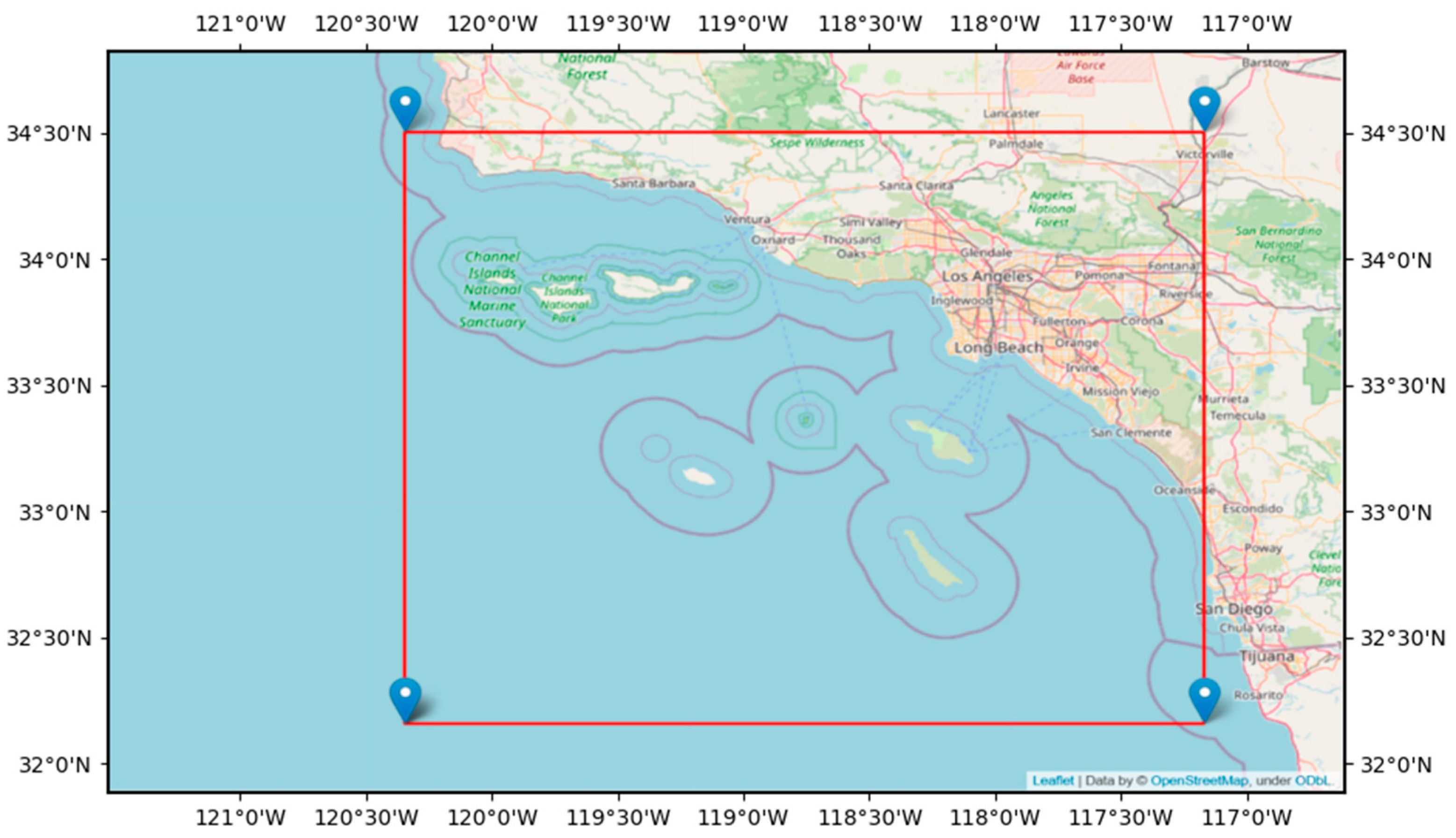
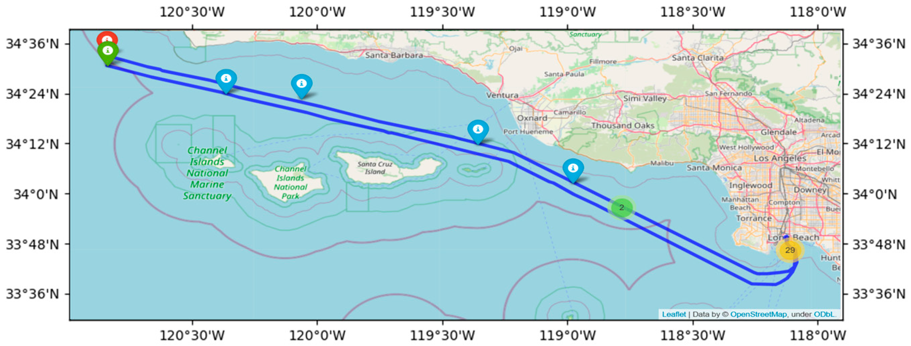
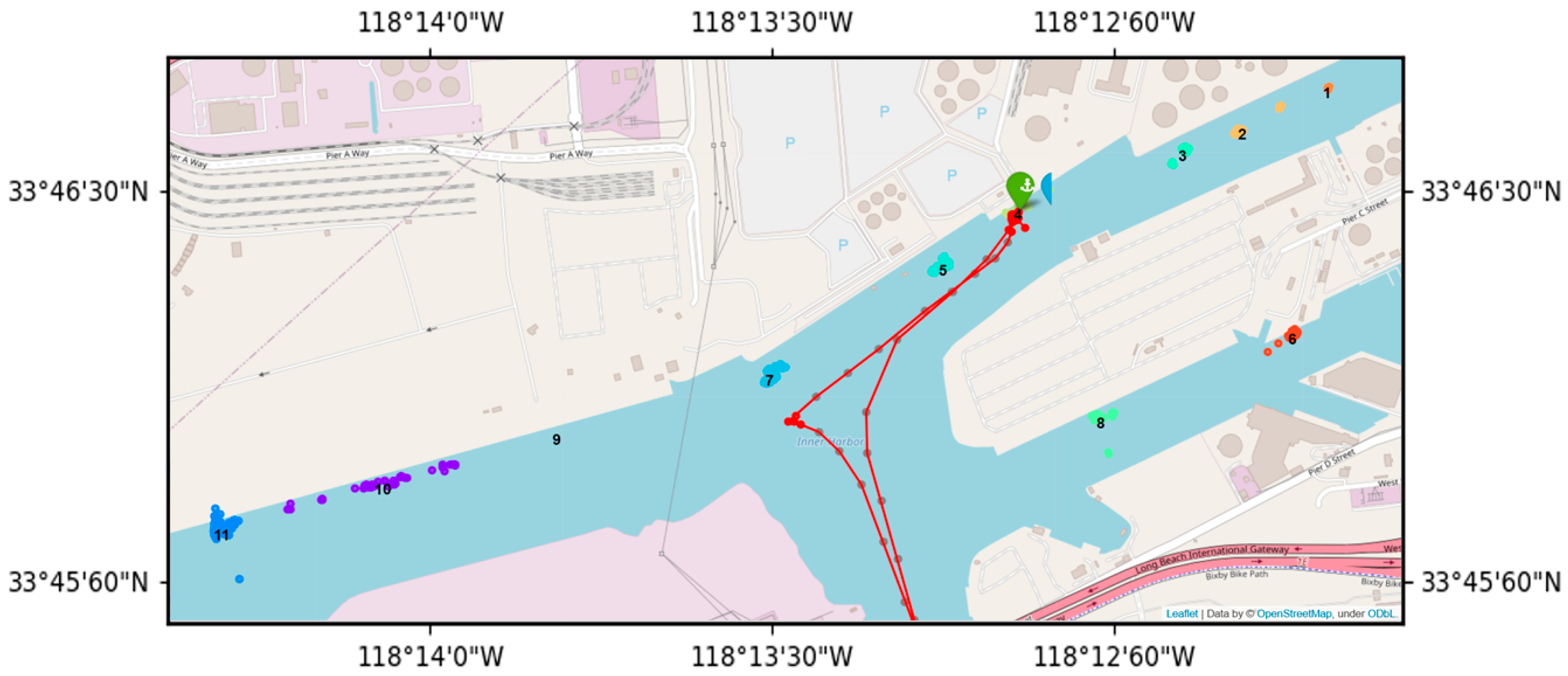
2.1. Research Area

The Port of Long Beach is one of the most important deep-water ports on the U.S. West Coast and one of the busiest container ports in the world. Located in Southern California near the city of Los Angeles, the Port of Long Beach serves as a key hub for U.S. foreign trade and plays a vital role in international trade and the global supply chain. With its modern infrastructure, an extensive network of shipping routes, and advanced cargo handling technology, the port efficiently processes goods from Asia, Latin America, and other regions, significantly driving economic development in California and the entire United States while also having a profound impact on the global trade system. The Port of Long Beach handles more than eight million TEUs (Twenty-foot Equivalent Units) annually, consistently ranking as the second-largest container port in the U.S., just behind the Port of Los Angeles. Covering an area of over 3200 hectares, the port features more than 70 berths and 22 container terminals, capable of accommodating and processing a large number of mega container ships simultaneously. Globally, the Port of Long Beach is regularly ranked among the top 20 container ports, earning a strong reputation for its efficient cargo handling capabilities and extensive network of shipping routes [34,35].

The AIS data for the Port of Long Beach, sourced from the website of the National Oceanic and Atmospheric Administration (NOAA), is utilized for the construction of the knowledge graph. AIS data include several types of information: Static information: Maritime Mobile Service Identity (MMSI), ship name, call sign, maximum static draught, vessel length, vessel width, and vessel type. Dynamic information: Coordinated Universal Time (UTC), longitude, latitude, course over ground (COG), speed over ground (SOG), Status, and Transceiver Class [36,37,38].

These AIS data messages essentially contain information related to a ship’s status during navigation, including both the vessel’s identity and its navigational position. The static information and dynamic information represent the vessel’s characteristics and its real-time location during navigation, respectively. By obtaining these two types of information, it is possible to uniquely identify a specific ship within a body of water. The AIS data types for vessels are as shown in

Table 1. Types of vessel AIS data.

Static Information	Dynamic Information
MMSI	UTC
ship name	longitude
call sign	latitude
maximum static draught	COG
vessel length	SOG
vessel width	heading
vessel type	Status
	Transceiver Class

.

Based on the ship’s purpose, vessels in a particular maritime area can be categorized into several types, including bulk carriers, liquid cargo ships (such as chemical tankers and oil tankers), passenger ships, container ships, roll-on/roll-off ships, and barges [39]. In AIS static data, the “vessel type” parameter predominantly encompasses the following categories: special-purpose ships, passenger ships, cargo ships, oil tankers, and other types of ships. These classifications correspond to the AIS message identifiers. The AIS codes for vessel types are as shown in

Table 2. AIS codes for vessel types.

Ship Type	AIS Main Ship Type Codes
Special-purpose ships	50–59
Passenger ships	60–69
Cargo ships	70–79
Oil tankers	80–89
Other types of ships	90–99

.

2.2. Methodology

2.2.1. AIS Data Preprocessing

This experiment collected 72 h of AIS data from the waters surrounding the Port of Long Beach, Los Angeles, as the basis for analyzing vessel navigation situation knowledge discovery. Additionally, a three-month dataset from a specific terminal within the Port of Long Beach was selected for berth knowledge discovery analysis. To ensure data quality and scientific validity, the raw data underwent stringent cleaning and correction procedures. The specific steps included removing all data records where the MMSI length was not 9 digits to exclude faulty or incorrectly identified records; Data entries with SOG values exceeding 30 knots or falling below 0 were removed, thereby minimizing the impact of outliers on the analysis of ship speed. Furthermore, records where the heading value was outside the 0–360 degrees range were removed to ensure the validity of heading data. Any records containing multiple outliers were also deleted to maintain dataset consistency and uniformity. These data-cleaning steps laid a solid foundation for the subsequent analysis [40,41].

To conduct an in-depth study of typical vessel navigation behaviors, this study focused primarily on cargo ship navigation data. The ship type field was strictly filtered, retaining only vessels with type codes between 70 and 79 to ensure the research was concentrated on cargo vessels. In addition, based on predefined latitude and longitude boundaries for the port area, a geospatial filter was applied to the AIS data to isolate vessels within the specified port region. This data processing not only effectively excluded non-target vessels but also ensured the spatial and behavioral consistency of the data, allowing for focused analysis of cargo vessel navigation dynamics [42,43].

In this study, vessels entering and exiting the port were chosen as the target sample, and only those with relatively complete trajectory data were selected for interpolation processing. To enhance the smoothness of the data, the Kalman filter was employed to process the AIS data of the target vessels [44]. Specifically, the latitude, longitude, SOG, and COG from the AIS data were used as the filter’s observations, while the state vector was assumed to consist of position and velocity. The Kalman filter combined the vessel’s motion model with actual observational data to smooth the trajectories and eliminate biases caused by sensor errors or environmental noise. During this process, the time interval was set to 1 min to ensure the accuracy and real-time performance of the smoothing process [45].

2.2.2. Vessel Navigation Knowledge Discovery

By analyzing AIS data, it is possible to effectively assess crossing, overtaking, and head-on situations between vessels. The key lies in the comprehensive analysis of key information such as SOG, COG, and latitude and longitude (LAT, LON). These factors are the primary basis for determining vessel situations. A crossing situation refers to a significant difference in the course of two vessels, with a potential point of intersection at a future moment [46]. The first step in determining a crossing situation is to calculate the course difference between the two vessels, analyzing whether there is sufficient deviation in their trajectories to predict a possible crossing. Here, ${\mathrm{C}\mathrm{O}\mathrm{G}}_1$ represents the course of the reference vessel and ${\mathrm{C}\mathrm{O}\mathrm{G}}_2$ represents the course of the target vessel. Assuming that calculations are performed in a planar coordinate system if the course difference $\Delta \mathrm{C}\mathrm{O}\mathrm{G}$ between the two vessels falls within 45° to 135°, this indicates a strong likelihood of a crossing situation. The specific formula can be found in Equation (1).

$$\Delta \mathrm{C}\mathrm{O}\mathrm{G}=\left|{\mathrm{C}\mathrm{O}\mathrm{G}}_1-{\mathrm{C}\mathrm{O}\mathrm{G}}_2\right|$$

(1)

By calculating the DCPA and the TCPA, the collision risk can be further assessed. The formula for calculating DCPA is provided in Equation (2), where $\mathrm{L}\mathrm{A}{\mathrm{T}}_1$, $\mathrm{L}\mathrm{O}{\mathrm{N}}_1$, $\mathrm{L}\mathrm{A}{\mathrm{T}}_2$, and $\mathrm{L}\mathrm{O}{\mathrm{N}}_2$ represent the latitude and longitude of the reference vessel and the target vessel, respectively. By combining the results of DCPA and TCPA calculations, a more accurate determination can be made regarding the potential for collision between the two vessels and the severity of the risk.

Furthermore, to determine when the two vessels will reach the closest point in the future, TCPA needs to be calculated. Calculating TCPA first requires determining the relative velocity vector between the two vessels, obtained by subtracting each vessel’s velocity vector from the other. The specific formula is shown in Equation (3), where ${\overrightarrow{\mathrm{V}}}_1$ and ${\overrightarrow{\mathrm{V}}}_2$ are the velocity vectors of each vessel, derived from their respective SOG and COG, and ${\overrightarrow{\mathrm{V}}}_{\mathrm{r}\mathrm{e}\mathrm{l}}$ represents the relative velocity vector between the vessels. In converting the course to vector components, a northward direction is taken as 0 degrees, increasing clockwise. Subsequently, the relative position vector between the vessels is calculated as specified in Equation (4). Using these vectors, TCPA can be computed by the formula shown in Equation (5), which calculates the time point when the rate of change in relative position between the vessels is at its minimum. A positive TCPA value indicates that the vessels will approach each other to the minimum distance at a future time, whereas a negative value suggests that the closest point has already passed [47].

$$\mathrm{D}\mathrm{C}\mathrm{P}\mathrm{A}=\sqrt{(\mathrm{L}\mathrm{A}{\mathrm{T}}_1-\mathrm{L}\mathrm{A}{\mathrm{T}}_2{)}^2+(\mathrm{L}\mathrm{O}{\mathrm{N}}_1-\mathrm{L}\mathrm{O}{\mathrm{N}}_2{)}^2}$$

(2)

$${\overrightarrow{\mathrm{V}}}_{\mathrm{r}\mathrm{e}\mathrm{l}}={\overrightarrow{\mathrm{V}}}_1-{\overrightarrow{\mathrm{V}}}_2$$

(3)

$${\overrightarrow{\mathrm{R}}}_{\mathrm{r}\mathrm{e}\mathrm{l}}=\left({\mathrm{L}\mathrm{O}\mathrm{N}}_2-{\mathrm{L}\mathrm{O}\mathrm{N}}_1,{\mathrm{L}\mathrm{A}\mathrm{T}}_2-{\mathrm{L}\mathrm{A}\mathrm{T}}_1\right)$$

(4)

$$\mathrm{T}\mathrm{C}\mathrm{P}\mathrm{A}=-{\displaystyle \frac{{\overrightarrow{\mathrm{R}}}_{\mathrm{r}\mathrm{e}\mathrm{l}}\cdot {\overrightarrow{\mathrm{V}}}_{\mathrm{r}\mathrm{e}\mathrm{l}}}{|{\overrightarrow{\mathrm{V}}}_{\mathrm{r}\mathrm{e}\mathrm{l}}{|}^2}}$$

(5)

An overtaking situation occurs when one vessel approaches and overtakes another from behind at a higher speed. In determining an overtaking situation, the first step is to calculate the course difference between the two vessels to assess whether they are on similar courses. Generally, if the course difference is less than 22.5°, the vessels can be considered to have aligned courses. Next, the relative speed is used to evaluate the rate at which the vessels are approaching each other, as calculated by Equation (6).

$$\Delta \mathrm{V}=\left|\mathrm{S}\mathrm{O}{\mathrm{G}}_1-\mathrm{S}\mathrm{O}{\mathrm{G}}_2\right|$$

(6)

Here, $\mathrm{S}\mathrm{O}{\mathrm{G}}_1$ and $\mathrm{S}\mathrm{O}{\mathrm{G}}_2$ represent the speeds of the two vessels, and $\Delta \mathrm{V}$ is the relative velocity between the reference vessel and the target vessel. By analyzing the relative velocity, the occurrence of an overtaking situation can be further assessed, as well as the time and distance involved in the overtaking process. If the relative velocity is greater than zero, the trailing vessel is catching up to the lead vessel, indicating an overtaking situation. In the case of a head-on situation, two vessels traveling in opposite directions with a course difference close to 180° can be considered to be in a head-on situation. If $\Delta \mathrm{C}\mathrm{O}\mathrm{G}$ is near 180°, the vessels are on a collision course. Additionally, by calculating DCPA and TCPA, the risk of collision in a head-on encounter can be further assessed. According to IMO Resolution A.422 and the COLREG Convention, a potential collision risk exists if the DCPA is less than 2 nautical miles or the TCPA is under 1 min.

A sliding window method is applied to AIS data to identify the acceleration and deceleration maneuvers of vessels. This approach captures short-term speed variations and enables detailed analysis of vessel dynamic behavior. Specifically, a fixed 10 min sliding window is set, and each window’s speed variation is calculated to identify any acceleration or deceleration events. To ensure detailed analysis at each time point in the time series, a sliding step of one minute is used. This means that the window advances by one minute each time, covering a new segment of data and allowing for continuous calculation and analysis across the entire time series. For each sliding window, the speed variation between the start and end points within the timeframe is calculated. The starting point of the window is designated as ${\mathrm{t}}_1$ and the endpoint as ${\mathrm{t}}_2$, with ${\mathrm{t}}_2-{\mathrm{t}}_1=10$ min. For the speed variation within this 10 min window, let $\mathrm{v}\left({\mathrm{t}}_1\right)$ be the speed at the starting time of the window and $\mathrm{v}\left({\mathrm{t}}_2\right)$ the speed at the endpoint. The speed change $\Delta \mathrm{v}$ can then be calculated using the formula in Equation (7).

$$\Delta \mathrm{v}=\mathrm{v}\left({\mathrm{t}}_2\right)-\mathrm{v}\left({\mathrm{t}}_1\right)$$

(7)

This formula provides an overview of the overall change in vessel speed within the window. Based on the calculated speed change $\Delta \mathrm{v}$, it is possible to determine whether acceleration or deceleration events have occurred. The specific criteria are as follows: when $\Delta \mathrm{v}>5$ knots, the event is classified as an acceleration event, indicating that the vessel’s speed has increased by more than 5 knots within the 10 min time window. Conversely, when $\Delta \mathrm{v}<-5$ knots, it signifies that the speed has decreased by more than 5 knots during that period, thus defining it as a deceleration event. Similarly, within each sliding window, the occurrence of a course change is assessed by calculating the change in heading between the start and end points of the window. Let the start time be denoted as ${\mathrm{t}}_1$ and the end time as ${\mathrm{t}}_2$, with the condition that ${\mathrm{t}}_2-{\mathrm{t}}_1=10$ min. The heading value at the start time, $\mathrm{H}\left({\mathrm{t}}_1\right)$, corresponds to the vessel’s heading at the beginning of the window, while $\mathrm{H}\left({\mathrm{t}}_2\right)$ represents the heading at the end time. The change in heading, $\Delta \mathrm{H}$, is expressed by the formula in Equation (8).

$$\Delta \mathrm{H}=\mathrm{H}\left({\mathrm{t}}_2\right)-\mathrm{H}\left({\mathrm{t}}_1\right)$$

(8)

To account for the cyclic nature of headings (i.e., from 0° to 360°), if the calculated heading change $\Delta \mathrm{H}$ exceeds 180°, adjustments need to be made. For example, when $\Delta \mathrm{H}>180°$, the heading change should be corrected using the formula $\Delta \mathrm{H}=\Delta \mathrm{H}-360°$. Conversely, when $\Delta \mathrm{H}<-180°$, the formula $\Delta \mathrm{H}=\Delta \mathrm{H}+360$ should be applied to ensure that the heading change reflects the shortest turning angle of the vessel. Based on the calculated heading change ΔH, a threshold can be set to identify turning events. For instance, when $\left|\Delta \mathrm{H}\right|>10°$, it is considered that the vessel made a significant turn within the time window. Specifically, if $\Delta \mathrm{H}>10°$, it is defined as a right-turn event; if $\Delta \mathrm{H}<-10°$, it is defined as a left-turn event. To comprehensively capture the dynamic behaviors of vessels, the sliding window begins at the starting point of the time series and progressively moves forward in 1 min increments. Each shift covers a new segment of data, allowing for the recalculation of speed and heading changes within that window. This stepwise sliding window approach enables continuous computation for each time point in the entire time series, ensuring that no acceleration, deceleration, or turning events are overlooked.

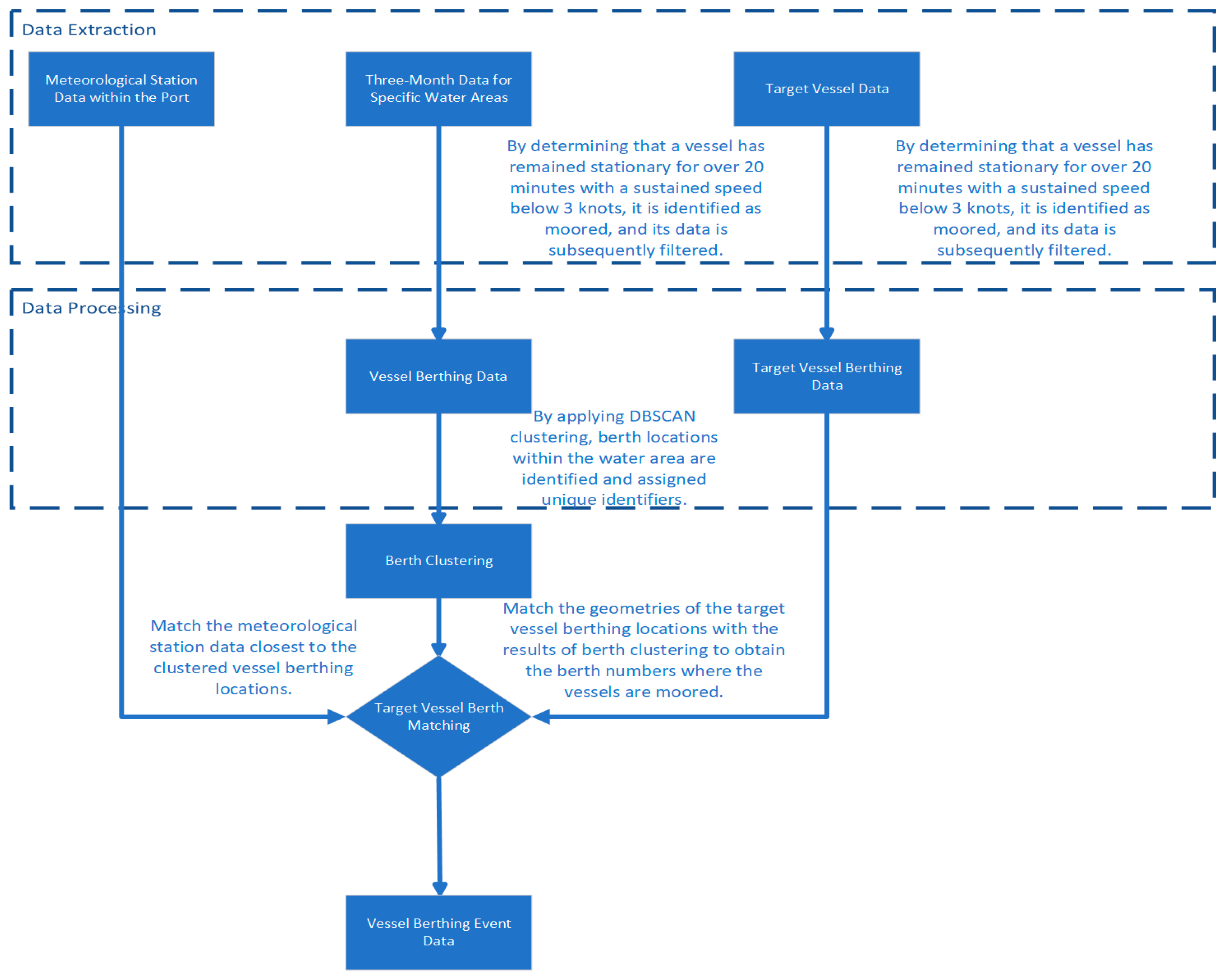
2.2.3. Berth Knowledge Discovery for Vessels

By filtering the cleaned AIS data, records with speeds below 3 knots are extracted to identify vessel mooring behavior, indicating that the vessels are in a low-speed state. The data for each vessel are then grouped, and mooring is determined based on time differences and vessel movement distances. Specifically, if a vessel’s speed remains below 3 knots for 10 min and its position shows little change, with a movement distance less than 0.0001 degrees (approximately 11 m), the vessel is marked as being in a moored state.

To determine the spatial distribution pattern of mooring points, the DBSCAN clustering analysis is employed. The DBSCAN effectively identifies nearby mooring points while excluding noise points. Since most vessels are currently under 400 m in length and their GPS units are installed on the compass deck towards the mid-to-rear section, we set the eps to 0.001 degrees to facilitate calculations. This establishes a clustering range with a radius of approximately 111 m. At the same berth, vessels are accurately grouped into a single cluster regardless of whether they are moored on the port or starboard side. Additionally, our experimental results have shown that this parameter setting yields effective outcomes. The DBSCAN algorithm recognizes areas with insufficient density as noise points. By setting min samples to 3, a point must have at least three neighboring points within a certain radius (eps) to be classified as a core point and form a cluster. This approach prevents isolated points from being mistakenly regarded as valid clusters and aids in filtering out outliers. After parameter settings are completed, the DBSCAN algorithm is applied to conduct a critical analysis of the extracted mooring points. DBSCAN clusters docking points that are sufficiently close and meet density criteria by examining the neighborhood of each point. Each cluster represents a potential mooring area or berth, while points aggregating into clusters are marked as noise points. The geometric center of each cluster is then calculated and designated as the mooring center’s location.

To identify the berth position of the vessels, an analysis of the target vessel’s behavioral data is conducted, particularly when the speed drops below 3 knots for more than 20 min, which typically indicates that the vessel is approaching or has already reached the berth. Based on this analysis, the nearest distance between the vessel’s position during this time period and predefined berth cluster points is calculated to determine the closest berth cluster, designating the corresponding dock as the vessel’s berth position. This process effectively combines vessel behavioral characteristics with geographical data, ensuring the accuracy of the berth position identification. Once the berth for the target vessel is determined, the geographical location information is used to find the nearest weather monitoring station in WeatherSpark, retrieving current weather information that primarily includes the temperature, wind speed, wind direction, and precipitation over the past two hours.

3. Results

3.1. Definitions of Vessel Navigation Entities and Relationships

In this experiment, data from a nearshore port area were selected, as 45.3% of maritime casualties and accidents occur in port areas, specifically during departure, arrival, and berthing or docking periods. The high density of vessels entering and leaving ports necessitates frequent maneuvers to avoid collisions [2]. Therefore, in this region, it is possible to detect a wide range of potential vessel events and information. The specific time range for the experimental data is from 29 March 2020 to 31 March 2020, with the spatial range defined as X Min = −120.792676, Y Min = 32.248706, X Max = −117.295349, and Y Max = 34.624237. The AIS data for vessels were cleaned and visualized to display the trajectories of all vessels in the area. Figure 1 illustrates the area from which the experimental data was extracted. The four blue markers indicate the corners of this data extraction region, and the red border lines delineate its boundaries. Mining the entity types and attributes in this area as shown in

Table 3. Entity types and attributes.

Entities	Attribute
Ship	MMSI, Vessel Type, Vessel Width, Vessel Length, Maximum Static Draught, COG, SOG
Navigation Event	Crossing Encounter, Head-on Encounter, Overtaking, Vessel Acceleration, Vessel Deceleration, Port Turn, Starboard Turn, Berthing, Departure from Berth
Berth	Berth Number
Weather Conditions	Wind speed, Wind Direction, Temperature, Precipitation Amount
Time	UTC

.

To identify vessels that had a complete record of entering the port, berthing, and departing during the period from 29 March 2020 to 31 March 2020, a port area filter was applied. The geographical boundaries were set to the red box region marked in Figure 2. X Min = −118.304224, Y Min = 33.705511, X Max = −118.163192, and Y Max = 33.777147. Vessels entering this port area with a vessel type code between 70 and 79 were considered cargo ships that had berthed in the port, as illustrated in Figure 2.

To develop a representative knowledge graph, we have selected a vessel that possesses comprehensive records of its port entry and exit activities. Through manual selection, a relatively complete vessel trajectory was chosen, which includes full information on entering and exiting the port. The vessel corresponding to this trajectory has the MMSI number 431816000. As shown in Figure 3, the red marker indicates the starting point of the recorded trajectory, while the green marker represents the endpoint.

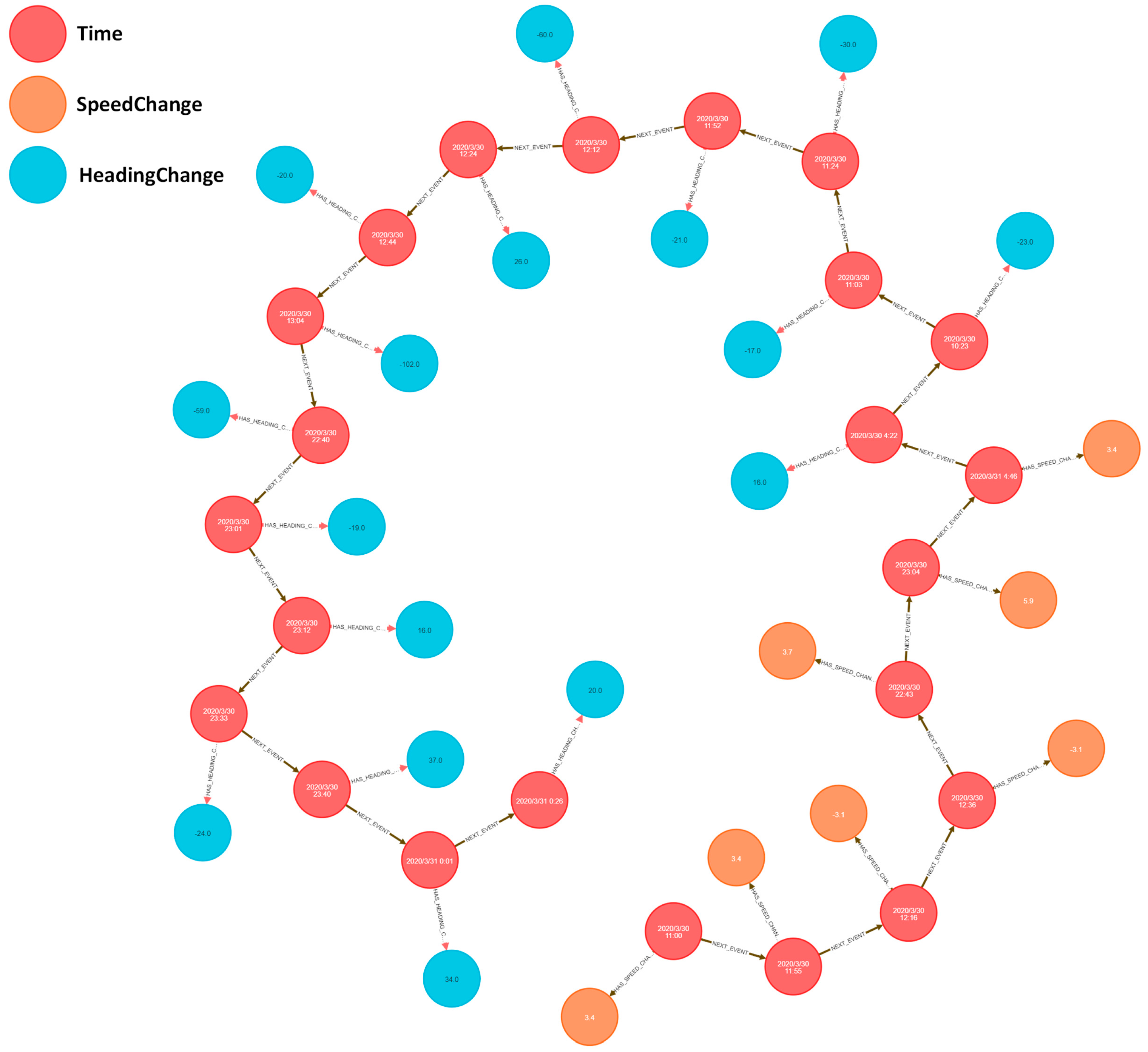
3.1.1. Extraction of Vessel Speed and Course Change Events

The data were loaded into a pre-built mathematical model, with the first step being the identification of acceleration, deceleration, and course change events for the target vessel. A sliding window method was used to analyze the vessel’s acceleration, deceleration, and turning events, and the results were visualized on an interactive map. The raw data containing the vessel’s trajectory were read from a CSV file, and the timestamp column was converted to a standard date and time format to ensure consistency in the time sequence. The data were then sorted chronologically to prepare for the sliding window analysis. To analyze the vessel’s acceleration and turning behavior, a sliding window was defined. The window size was set to 10 min, with a 1 min step. This means that each sliding window covered the vessel’s trajectory data for 10 min, ensuring that dynamic behavior during each period was captured. To identify acceleration and deceleration events, the speed change between the start and end of each window was calculated. If the speed increased or decreased by more than five knots, it was recorded as an acceleration or deceleration event. Turning events were identified based on the change in course, with heading changes exceeding 180° corrected to ensure accurate angle calculations. A course change of more than 15° was defined as a turning event. After identifying the events, the vessel’s trajectory, as well as acceleration, deceleration, and turning events, was visualized. On the map, the locations of acceleration and deceleration events were marked, with green representing acceleration, red representing deceleration, and orange used to mark turning events. Figure 4 illustrates the vessel’s acceleration, deceleration, and turning events. The orange markers represent turning events, the red markers indicate deceleration events, and the green markers signify acceleration events.

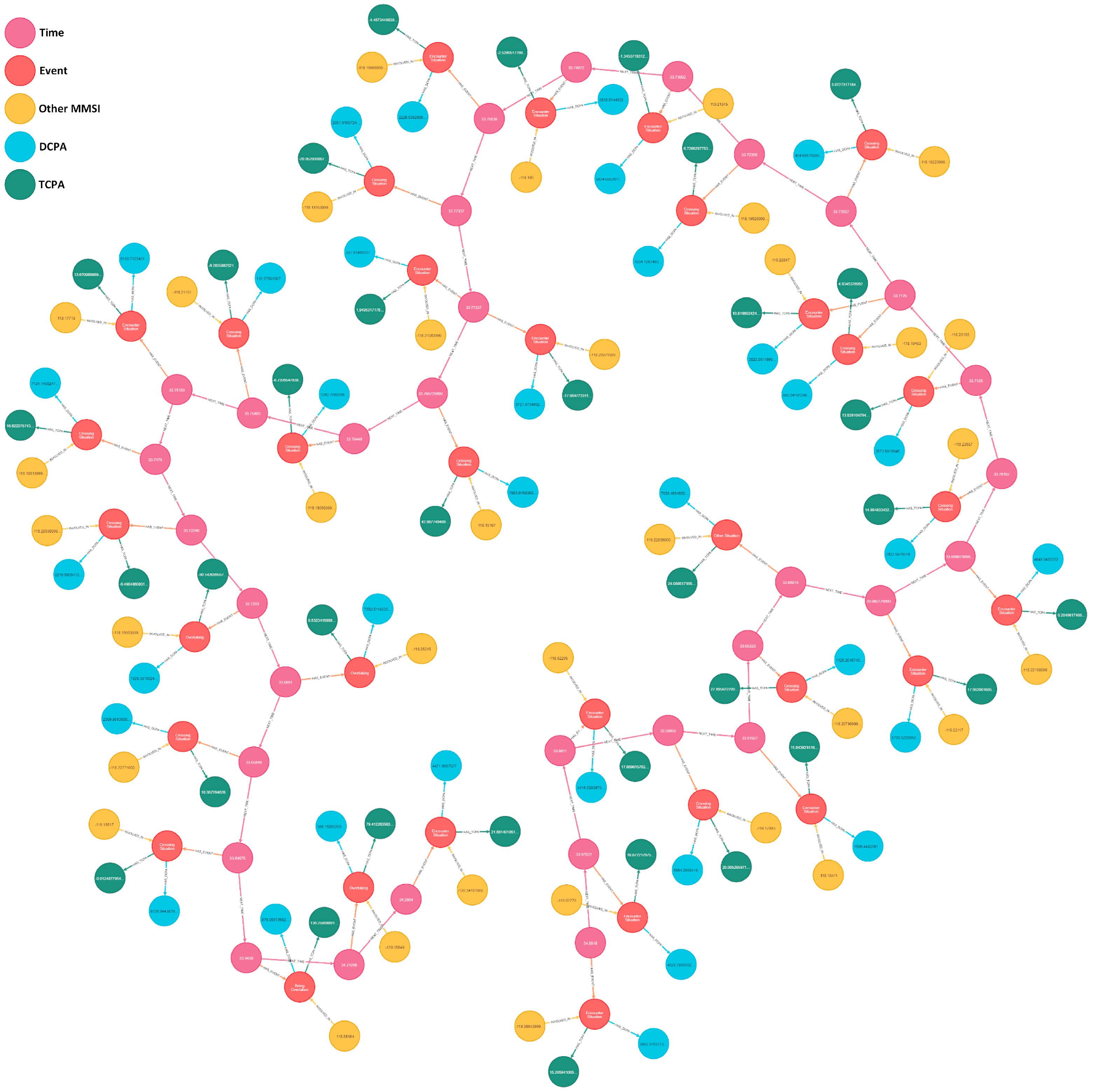
3.1.2. Extraction of Vessel Encounter Events

This analysis examines the navigational situations encountered by the vessel with MMSI 431816000 during its entry and exit from the port in relation to other nearby vessels. From the navigational data, trajectory points meeting specific conditions are selected by identifying points from other vessels within a two-nautical-mile range of MMSI 431816000. This filtering reduces irrelevant data and lowers the computational load by screening the timestamps in all AIS data. Only data points within 30 min before the start time and 30 min after the end time of MMSI 431816000’s movement are retained. To ensure the accuracy of subsequent calculations, latitude and longitude data must be converted from degrees to radians, as the BallTree data structure requires input in radians. The conversion formulas for latitude and longitude are provided in Equations (9) and (10).

$$LA{T}_{\mathrm{r}\mathrm{a}\mathrm{d}}=LAT\times {\displaystyle \frac{\pi }{180}}$$

(9)

$$LO{N}_{\mathrm{r}\mathrm{a}\mathrm{d}}=LON\times {\displaystyle \frac{\pi }{180}}$$

(10)

In this context, $LAT$ and $LON$ represent the latitude and longitude from the original data, while $LA{T}_{\mathrm{r}\mathrm{a}\mathrm{d}}$ and $LO{N}_{\mathrm{r}\mathrm{a}\mathrm{d}}$ are the corresponding values converted into radians. The experiment filtered the target vessel’s data from all available records. To efficiently locate neighboring points around the trajectory points of the target vessel, the experiment employed the BallTree spatial search algorithm. This algorithm can quickly find nearby points on a sphere. BallTree uses the Haversine formula to calculate the great-circle distance between two points. The search range was set to two nautical miles, which was then converted into radians, since the Earth’s radius is approximately 3440.065 nautical miles. The conversion formula from nautical miles to radians is given in Equation (11).

$$\mathrm{r}={\displaystyle \frac{2}{3440.065}}$$

(11)

This formula converts a distance of two nautical miles into spherical radians, allowing for spatial queries within the BallTree. Next, the spherical distance between two points is calculated using the Haversine formula, as shown in Equation (12).

$$d_{\mathrm{h}}=2R\cdot \arcsin \left(\sqrt{{\mathit{sin}}^2\left({\displaystyle \frac{\Delta \varphi }{2}}\right)+\mathit{cos}\left({\varphi }_1\right)\cdot \mathit{cos}\left({\varphi }_2\right)\cdot {\mathit{sin}}^2\left({\displaystyle \frac{\Delta \lambda }{2}}\right)}\right)$$

(12)

Here, $d_{\mathrm{h}}$ represents the Haversine distance between two points in radians; $R$ is the Earth’s radius; $\Delta \varphi ={\varphi }_2-{\varphi }_1$ is the latitude difference between the two points; $\Delta \lambda ={\lambda }_2-{\lambda }_1$ is the longitude difference between the two points. ${\varphi }_1,{\varphi }_2$ denote the latitudes of the two points, while ${\lambda }_1, {\lambda }_2$ denote the longitudes. This formula is used to calculate the distance from each trajectory point of the reference vessel to all trajectory points of other vessels.

Using this formula, all points within two nautical miles of each trajectory point are calculated. Using the BallTree. query_radius method, the experiment queried each trajectory point of the target vessel to retrieve all other points within a two-nautical-mile radius. Each set of nearby points identified through the queries was stored in a results list. The results list was then merged into a single database. Since vessels might occupy the same spatial position at different times but still be within two nautical miles of each other, duplicate entries were removed. After filtering based on distance, the current AIS data consisted of the target vessel’s trajectory points and those within two nautical miles of the target vessel’s trajectory. However, since vessel encounters are events that occur in the same time and space, an additional filter was applied, focusing on both time and space. This filter selected data where the time difference between the target vessel’s trajectory points and the other vessels’ points was less than 2 min, and the distance was less than two nautical miles. As shown in Figure 5, the green marker denotes the starting point of the ship’s trajectory, the red marker indicates its endpoint and the blue markers represent events where the ship was within two nautical miles of another vessel.

The final vessel encounter data are used to identify the navigational situation of the target vessel. By analyzing the COG and SOG of both vessels, the relationship between them is determined, allowing us to assess whether the navigational situation is a head-on encounter, crossing encounter, overtaking, or another scenario. Additionally, for each encounter, the DCPA and TCPA are calculated to assess the urgency of the vessel encounter situation.

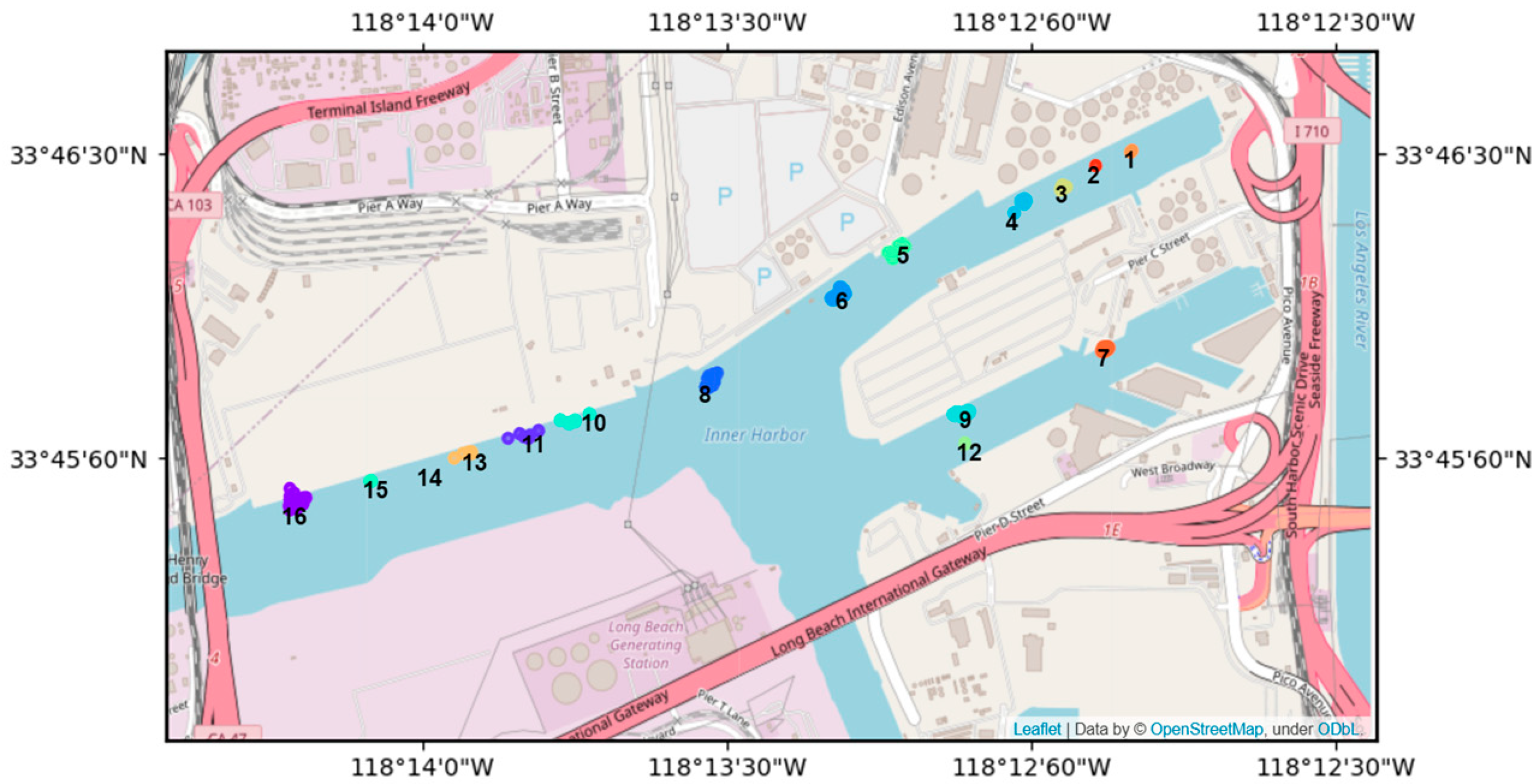
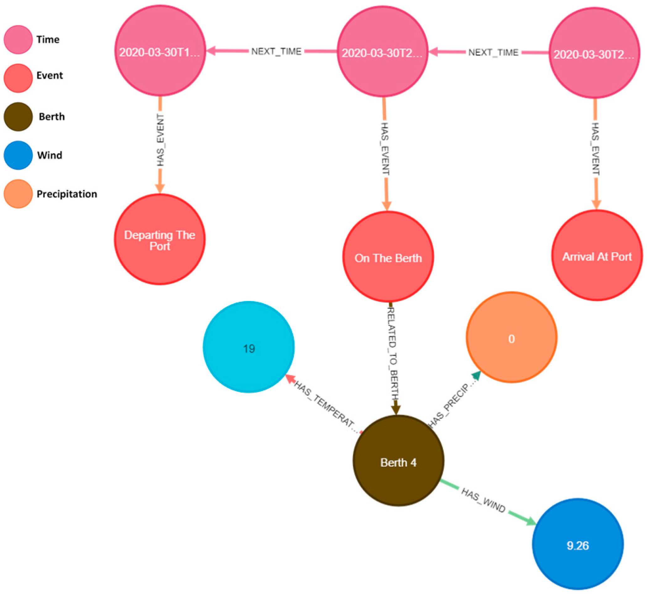
3.1.3. Extraction of Vessel Berthing Events

Specifically, the port water areas are predefined. When a vessel enters this designated area, it is recorded as an arrival event. The vessel’s speed, positional movement distance, and dwell time are then used as criteria to identify records where the vessel remains in a particular location for an extended period with minimal movement, categorizing these as berthing events. After a period of berthing, when the vessel’s SOG remains below three knots and begins to change, this moment is logged as a departure event. The departure event concludes when the vessel exits the defined port water area [48]. The specific extraction process of vessel berthing events can be seen in Figure 6.

For each vessel’s unique identifier, the MMSI, the time difference between consecutive records, is calculated, and latitude and longitude are used to determine the vessel’s movement distance during each interval. Points where the speed is below three knots, and the movement distance remains nearly unchanged within a 20 min timeframe are marked as “berthing points”. This marking method effectively identifies vessels that remain at the dock or a specific location for an extended period. The density clustering algorithm DBSCAN is then applied to the identified berthing points for clustering analysis. DBSCAN aggregates nearby berthing points into clusters by setting a radius (eps = 0.001 degrees) and a minimum sample size (min_samples = 3) while ignoring potential noise points. Each cluster represents the distribution of berthing points for vessels in different locations. From each cluster, a representative point is selected and sorted by latitude from north to south to visually present the distribution of vessels across various berthing areas. Finally, the folium library is utilized to visualize the berthing points and clustering results. Each berthing point is assigned a different color to distinguish between various clusters, and numbered labels are added to the representative points of each cluster. The resulting vessel berth clustering is illustrated in Figure 7.

To determine the geometric center of each cluster, the average latitude and longitude of all berthing points within the cluster are calculated, designating this center as the representative point for the berths. This representative point is used for subsequent trajectory-matching operations. The distance between the target vessel’s low-speed trajectory points (defined as points with speeds less than 3 knots) and these berth representative points are assessed to identify the nearest berth. Each low-speed trajectory point of the target vessel is iterated by querying the nearest distance to all berth representative points using BallTree. The distance between each low-speed trajectory point and the nearest berth point is recorded, along with the corresponding berth index, thereby documenting the matching relationship between the berth and the low-speed trajectory point. Subsequently, the number of matches for each berth is tallied. Whenever a low-speed trajectory point finds its nearest berth, the match count for that berth is incremented. Among all berths, the one with the highest number of trajectory point matches is considered the final berthing point for the vessel, identifying the berth with the most matches. Green denotes the ship’s final berthing position. The identification of vessel berthing points is illustrated in Figure 8.

Once the berthing point for the target vessel is determined, the current weather information is retrieved from the nearest weather monitoring station to its geographical location in WeatherSpark. The key meteorological data include the temperature, wind speed, wind direction, and precipitation over the past two hours [49].

4. Discussion

4.1. Maritime Traffic Knowledge Construction

To analyze the pre-saved triples file containing vessel speed and heading change events, the vessel encounter data are first read, and the timestamp field is processed to ensure the data are ordered chronologically. This organized data will ultimately be stored in a Neo4j graph database to support future data storage. For each speed and heading change event, event nodes are created in the graph database. These nodes include attributes such as “start time”, “end time”, “event type”, “speed change”, “latitude”, “longitude”, and “heading change”. These data represent various events that occur within a specific timeframe, capturing the vessel’s speed and heading changes, as well as geographical coordinate information, as explained in

Table 4. The node and relationship of vessel heading and speed changes.

Node Labels	Relationship Types
Event	NEXT_EVENT
Speed Change	HAS_ Speed_ Change
Heading Change	HAS_ Heading_ Change

. In cases of speed and heading changes, corresponding nodes for speed changes and heading changes are created, connecting them to the relevant event nodes through relationships. Additionally, events are categorized into speed changes and heading changes, with positive values assigned for acceleration events and negative values for deceleration events. Similarly, right turns are assigned positive values, while left turns are assigned negative values, which are all noted in the attributes of each event. The time knowledge graph of vessel heading and speed changes is shown in Figure 9.

In Neo4j, nodes representing time are created, with corresponding attributes added to these time nodes based on properties such as target latitude, longitude, speed, and heading from the triples. Next, an Other MMSI node is created to record relevant latitude, longitude, speed, and heading information. Vessel encounter event nodes are then established in Neo4j and connected to the time nodes and Other MMSI nodes through relationships (HAS_EVENT and INVOLVED_IN). Additionally, the DCPA and TCPA nodes are linked to the event nodes through relationships (HAS_DCPA and HAS_TCPA). To ensure the sequential relationship between the time nodes, logic is included to handle the time series, as explained in

Table 5. The node and relationship of Vessel Navigation Encounters.

Node Labels	Relationship Types
Time	NEXT_TIME
Other MMSI	INVOLVED_IN
Event	HAS_EVENT
DCPA	HAS_DCPA
TCPA	HAS_TCPA

. If the current time does not match the previous time node, a NEXT_TIME relationship is created between the two time nodes to maintain the integrity of the temporal sequence in the knowledge graph. The knowledge graph of vessel navigation encounters is illustrated in Figure 10.

The provided triples include nodes such as berths, temperature, wind, precipitation, and time. These nodes represent relevant information and environmental conditions at specific time points during the vessel’s entry and exit from the port. Relationships between the nodes are defined, interconnecting them to form a meaningful knowledge structure. During the vessel’s arrival and departure periods, three main event nodes are established: name: Arrival At Port; name: On The Berth; name: Departing The Port, linking these events to their corresponding event nodes, as explained in

Table 6. The node and relationship of Vessel Arrival and Departure Events.

Node Labels	Relationship Types
Berth	RELATED_TO_BERTH
Temperature	HAS_TEMPERATURE
Wind	HAS_WIND
Precipitation	HAS_PRECIPITATION
Time	NEXT_TIME
Event	HAS_EVENT

. Additionally, the specific berth of the On The Berth event is associated, and the climatic conditions at the port, such as temperature, precipitation, and wind, are linked with the berth. This constructs a comprehensive knowledge graph of the vessel’s complete arrival and departure events, as illustrated in Figure 11.

By sorting the timestamps of all vessel navigation events, time nodes are progressively created, establishing temporal relationships among them to form a “time chain (NEXT)” that describes the sequence of events. Corresponding event nodes are then created based on different types of scenarios, such as “encounter situations”, “overtaking”, “crossing situations”, and “passing”, and these nodes are connected to the time nodes. Specific attribute nodes are added as needed, such as DCPA” and TCPA. “For berth operation events, the berth nodes are connected using the “At Berth (AT_BERTH)” relationship. For operational changes such as “acceleration”, “deceleration”, “left turn”, “right turn”, “Speed Change (Speed Change)”, and “Course Change (Course Change)” nodes are used to describe these actions. During the vessel’s arrival and departure periods, three main event nodes are established: “Arrival At Port”, “On The Berth”, and “Departing The Port”, linking these events to the corresponding berth, time, and climatic conditions. This constructs a comprehensive knowledge graph of the vessel’s arrival and departure events, as illustrated in Figure 12.

4.2. Maritime Traffic Knowledge Discovery

During a ship’s voyage, many events are intrinsically connected, though these connections may not be readily apparent. Knowledge graphs can represent complex entities and their relationships in a structured and semantic manner, enabling a comprehensive expression of associations among multi-source heterogeneous data. Moreover, they allow for reasoning to uncover hidden knowledge, such as inferring congestion causes or identifying critical nodes in the transportation domain. Here, we utilized the Cypher query language in Neo4j to analyze two non-adjacent time nodes, 30 March 2020 12:12:00 and 30 March 2020 23:01:00. By exploring the connection paths between these two time nodes, we aimed to uncover implicit information hidden within them. Given that the number of possible paths between nodes in a complex knowledge graph can approach infinity, we limited the number of intermediate nodes to fewer than six to constrain the number of discovered paths. as illustrated in Figure 13.

Additionally, it is possible to query two different events to uncover the relationships between them. For example, by querying the “Turns to port” event and the “Crossing Situation” event, we aim to identify their connections. Similarly, to limit the number of discovered paths, we set the number of intermediate nodes to three in this case, as illustrated in Figure 14.

In Figure 13, it is evident that the ship experienced “Turns to port” events at both 30 March 2020 12:12:00 and 30 March 2020 23:01:00. Figure 14 shows that “Turns to port” and “Crossing Situation” events frequently occur at adjacent time nodes. This observation aligns well with real-world maritime navigation, where ships often need to execute turning maneuvers during crossing situations to ensure safe navigation.

5. Conclusions

The temporal knowledge graph effectively models the complex relationships of vessels, such as encounters, crossing situations, and overtaking, providing rich semantic information that aids vessels in making intelligent decisions when faced with sudden events. By incorporating temporal information, the knowledge graph not only reflects the current vessel situation but also enables trend predictions, such as collision warnings and route planning, thereby enhancing the system’s intelligence level. Furthermore, this study not only relies on AIS data but also semantically fuses meteorological data with dynamic vessel data to construct a more comprehensive temporal knowledge graph. This fusion of multi-source data enables smart vessels to understand their own navigation status as well as that of other vessels, allowing for more complex reasoning and decision-making in response to changes in the marine environment.

By utilizing sliding window techniques and the DBSCAN clustering algorithm, this study can automatically identify key events during vessel navigation (such as acceleration, deceleration, turning, and encounters) and model them as dynamic event nodes within the knowledge graph. This event identification and modeling approach significantly enhances the automation and data processing capabilities of the system. Integrating dynamic event modeling within the knowledge graph not only captures vessel behaviors but also facilitates intelligent situational analysis and reasoning, providing technical assurance for safe navigation. Moreover, the proposed method is applicable not only to the dynamic data processing of individual vessels but can also be extended to monitor and perceive large-scale groups of vessels. Through efficient data preprocessing and event identification processes, the system maintains high processing performance even when confronted with a large volume of real-time vessel data. The system exhibits excellent scalability capable of handling extensive vessel datasets while performing effectively in complex ports or densely trafficked shipping areas, supporting global monitoring and situational analysis for multiple vessels. It can also flexibly adapt to different marine areas and port environments by dynamically adjusting event identification and modeling parameters, ensuring efficient performance under various conditions. The proposed method for constructing a temporal knowledge graph provides strong data and decision support for the autonomous navigation of smart vessels. Through the knowledge graph, the system can automatically identify potential risks and environmental changes, reducing human errors in operations and enhancing the automated navigation capabilities of vessels. The temporal knowledge graph offers real-time, comprehensive situational awareness, assisting vessels in autonomously responding to complex navigation conditions.

Although the proposed knowledge graph construction method based on multi-source data has shown promising results in supporting situational awareness for intelligent ships, there are still some shortcomings that require further improvement and optimization. Firstly, while this study integrates AIS data and meteorological data, other critical data sources—such as radar data, satellite imagery, and ship automatic navigation system information—have yet to be fully incorporated. Comprehensive fusion of multi-source heterogeneous data is essential for intelligent ships to achieve a more accurate understanding of complex environments. Moreover, this study primarily focuses on proposing a method for constructing a maritime traffic knowledge graph. However, the limited dataset results in constrained information discovery, underscoring the need for larger datasets to enable more robust knowledge extraction.

The construction of the temporal knowledge graph partially supports the modeling and expression of dynamic events. However, due to the high real-time requirements of vessel navigation data, achieving efficient real-time updates of the knowledge graph remains a challenge. AIS data are characterized by high-frequency dynamics, and when handling these dynamic changes, the knowledge graph requires a more flexible and efficient updating mechanism; otherwise, it may struggle to meet the real-time demands of practical applications. In large-scale vessel navigation scenarios, the vast amount of data and complex environments may pose challenges to the scalability of the knowledge graph and the adaptability of the system. Maintaining efficient storage, retrieval, and analysis performance under massive data conditions, as well as adapting to different vessel behavior patterns in various marine areas and port environments, requires further optimization and enhancement.

References

1. Xin, X.; Liu, K.; Loughney, S.; Wang, J.; Li, H.; Ekere, N.; Yang, Z. Multi-scale collision risk estimation for maritime traffic in complex port waters. Reliab. Eng. Syst. Saf. 2023, 240, 109554. [Google Scholar] [CrossRef]
2. Hwang, T.; Youn, I.H. Collision Risk Situation Clustering to Design Collision Avoidance Algorithms for Maritime Autonomous Surface Ships. J. Mar. Sci. Eng. 2022, 10, 1381. [Google Scholar] [CrossRef]
3. Chen, X.Q.; Chen, W.P.; Wu, B.; Wu, H.F.; Xian, J.F. Ship visual trajectory exploitation via an ensemble instance segmentation framework. Ocean Eng. 2024, 313, 119368. [Google Scholar] [CrossRef]
4. Zhang, K.; Huang, L.W.; He, Y.X.; Wang, B.; Chen, J.H.; Tian, Y.F.; Zhao, X.Y. A real-time multi-ship collision avoidance decision-making system for autonomous ships considering ship motion uncertainty. Ocean Eng. 2023, 278, 114205. [Google Scholar] [CrossRef]
5. Gao, P.; Zhou, L.; Zhao, X.; Shao, B. Research on ship collision avoidance path planning based on modified potential field ant colony algorithm. Ocean Coast. Manag. 2023, 235, 106482. [Google Scholar] [CrossRef]
6. Filipiak, D.; Wecel, K.; Strózyna, M.; Michalak, M.; Abramowicz, W. Extracting Maritime Traffic Networks from AIS Data Using Evolutionary Algorithm. Bus. Inf. Syst. Eng. 2020, 62, 435–450. [Google Scholar] [CrossRef]
7. Liu, T.; Ma, J.W. Ship Navigation Behavior Prediction Based on AIS Data. IEEE Access 2022, 10, 47997–48008. [Google Scholar] [CrossRef]
8. Kim, J.S.; Park, H.J.; Shin, W.; Park, D.; Han, S.W. WAY: Estimation of Vessel Destination in Worldwide AIS Trajectory. IEEE Trans. Aerosp. Electron. Syst. 2023, 59, 5961–5977. [Google Scholar] [CrossRef]
9. Huang, I.L.; Lee, M.C.; Nieh, C.Y.; Huang, J.C. Ship Classification Based on AIS Data and Machine Learning Methods. Electronics 2024, 13, 98. [Google Scholar] [CrossRef]
10. Chen, W.J.; Chen, J.H.; Geng, J.J.; Ye, J.; Yan, T.; Shi, J.; Xu, J.H. Monitoring and evaluation of ship operation congestion status at container ports based on AIS data. Ocean Coast. Manag. 2023, 245, 106836. [Google Scholar] [CrossRef]
11. D’Afflisio, E.; Braca, P.; Willett, P. Malicious AIS Spoofing and Abnormal Stealth Deviations: A Comprehensive Statistical Framework for Maritime Anomaly Detection. IEEE Trans. Aerosp. Electron. Syst. 2021, 57, 2093–2108. [Google Scholar] [CrossRef]
12. Huang, Y.; Chen, L.; Chen, P.; Negenborn, R.R.; van Gelder, P.H.A.J.M. Ship collision avoidance methods: State-of-the-art. Saf. Sci. 2020, 121, 451–473. [Google Scholar] [CrossRef]
13. Murray, B.; Perera, L.P. Ship behavior prediction via trajectory extraction-based clustering for maritime situation awareness. J. Ocean Eng. Sci. 2022, 7, 1–13. [Google Scholar] [CrossRef]
14. Wang, Q.; Zhang, Q.; Wang, Y.; Hu, Y.; Guo, S. Event-triggered adaptive finite time trajectory tracking control for an underactuated vessel considering unknown time-varying disturbances. Transp. Saf. Environ. 2023, 5, tdac078. [Google Scholar] [CrossRef]
15. Ha, J.; Roh, M.I.; Lee, H.W. Quantitative calculation method of the collision risk or collision avoidance in ship navigation using the CPA and ship domain. J. Comput. Des. Eng. 2021, 8, 894–909. [Google Scholar] [CrossRef]
16. Wang, Y.; Perera, L.P.; Batalden, B.-M. Localized advanced ship predictor for maritime situation awareness with ship close encounter. Ocean Eng. 2024, 306, 117704. [Google Scholar] [CrossRef]
17. Chen, X.; Wu, H.; Han, B.; Liu, W.; Montewka, J.; Liu, R.W. Orientation-aware ship detection via a rotation feature decoupling supported deep learning approach. Eng. Appl. Artif. Intell. 2023, 125, 106686. [Google Scholar] [CrossRef]
18. Ju, M.R.; Niu, B.; Hu, Q. SARGAN: A Novel SAR Image Generation Method for SAR Ship Detection Task. IEEE Sens. J. 2023, 23, 28500–28512. [Google Scholar] [CrossRef]
19. Liu, J.; Liu, L.; Xiao, J.R. Ellipse Polar Encoding for Oriented SAR Ship Detection. IEEE J. Sel. Top. Appl. Earth Obs. Remote Sens. 2024, 17, 3502–3515. [Google Scholar] [CrossRef]
20. Xu, X.Q.; Wu, B.; Xie, L.; Teixeira, A.P.; Yan, X.P. A Novel Ship Speed and Heading Estimation Approach Using Radar Sequential Images. IEEE Trans. Intell. Transp. Syst. 2023, 24, 11107–11120. [Google Scholar] [CrossRef]
21. Wu, Y.; Chu, X.M.; Deng, L.; Lei, J.Y.; He, W.; Królczyk, G.; Li, Z. A new multi-sensor fusion approach for integrated ship motion perception in inland waterways. Measurement 2022, 200, 111630. [Google Scholar] [CrossRef]
22. Liu, W.W.; Liu, Y.C.; Gunawan, B.A.; Bucknall, R. Practical Moving Target Detection in Maritime Environments Using Fuzzy Multi-sensor Data Fusion. Int. J. Fuzzy Syst. 2021, 23, 1860–1878. [Google Scholar] [CrossRef]
23. Jiang, J.H.; Zuo, Y.; Xiao, Y.; Zhang, W.J.; Li, T.S. STMGF-Net: A Spatiotemporal Multi-Graph Fusion Network for Vessel Trajectory Forecasting in Intelligent Maritime Navigation. IEEE Trans. Intell. Transp. Syst. 2024, 25, 21367–21379. [Google Scholar] [CrossRef]
24. Xiao, Y.; Li, X.C.; Yin, J.J.; Liang, W.; Hu, Y.P. Adaptive multi-source data fusion vessel trajectory prediction model for intelligent maritime traffic. Knowl. -Based Syst. 2023, 277, 110799. [Google Scholar] [CrossRef]
25. Liu, X.; Tang, J.; Yuan, C.; Gao, F.; Ding, X. Examining the characteristics between time and distance gaps of secondary crashes. Transp. Saf. Environ. 2023, 6, tdad014. [Google Scholar] [CrossRef]
26. Bi, Z.; Cheng, S.Y.; Chen, J.; Liang, X.Z.; Xiong, F.Y.; Zhang, N.Y. Relphormer: Relational Graph Transformer for Knowledge Graph Representations. Neurocomputing 2024, 566, 127044. [Google Scholar] [CrossRef]
27. Peng, C.Y.; Xia, F.; Naseriparsa, M.; Osborne, F. Knowledge Graphs: Opportunities and Challenges. Artif. Intell. Rev. 2023, 56, 13071–13102. [Google Scholar] [CrossRef]
28. Guan, N.N.; Song, D.D.; Liao, L.J. Knowledge graph embedding with concepts. Knowl. -Based Syst. 2019, 164, 38–44. [Google Scholar] [CrossRef]
29. Liu, W.Q.; Liu, J.; Wu, M.M.; Abbas, S.; Hu, W.; Wei, B.F.; Zheng, Q.H. Representation learning over multiple knowledge graphs for knowledge graphs alignment. Neurocomputing 2018, 320, 12–24. [Google Scholar] [CrossRef]
30. Hu, J.L.; Zhou, W.X.; Zheng, P.J.; Liu, G.Y. A Novel Approach for the Analysis of Ship Pollution Accidents Using Knowledge Graph. Sustainability 2024, 16, 5296. [Google Scholar] [CrossRef]
31. Xie, C.X.; Zhang, L.M.; Zhong, Z.G. A Novel Method for Constructing Spatiotemporal Knowledge Graph for Maritime Ship Activities. Electronics 2023, 12, 3205. [Google Scholar] [CrossRef]
32. Zhang, Y.T.; Xu, R.Q.; Lu, W.P.; Mayer, W.; Ning, D.; Duan, Y.C.; Zeng, X.; Feng, Z.W. Multi-Modal Spatio-Temporal Knowledge Graph of Ship Management. Appl. Sci. 2023, 13, 9393. [Google Scholar] [CrossRef]
33. Tamasauskaite, G.; Groth, P. Defining a Knowledge Graph Development Process Through a Systematic Review. ACM Trans. Softw. Eng. Methodol. 2023, 32, 27. [Google Scholar] [CrossRef]
34. Knatz, G. Port mergers: Why not Los Angeles and Long Beach? Res. Transp. Bus. Manag. 2018, 26, 26–33. [Google Scholar] [CrossRef]
35. Gu, B.M.; Liu, J.G.; Ye, X.H.; Gong, Y.; Chen, J.H. Data-driven approach for port resilience evaluation. Transp. Res. Part E Logist. Transp. Rev. 2024, 186, 103570. [Google Scholar] [CrossRef]
36. Wang, C.L.; Han, P.H.; Zhu, M.D.; Osen, O.; Zhang, H.X.; Li, G.Y. AIS Data-Based Hybrid Predictor for Short-Term Ship Trajectory Prediction Considering Uncertainties. IEEE Trans. Intell. Transp. Syst. 2024, 25, 20268–20279. [Google Scholar] [CrossRef]
37. Guan, M.; Cao, Y.; Cheng, X. Research of AIS Data-Driven Ship Arrival Time at Anchorage Prediction. IEEE Sens. J. 2024, 24, 12740–12746. [Google Scholar] [CrossRef]
38. Duan, Y.S.; Huang, J.Q.; Lei, J.L.; Kong, L.H.; Lv, Y.B.; Lin, Z.L.; Chen, G.H.; Khan, M.K. AISChain: Blockchain-Based AIS Data Platform With Dynamic Bloom Filter Tree. IEEE Trans. Intell. Transp. Syst. 2023, 24, 2332–2343. [Google Scholar] [CrossRef]
39. Sciancalepore, S.; Tedeschi, P.; Aziz, A.; Di Pietro, R. Auth-AIS: Secure, Flexible, and Backward-Compatible Authentication of Vessels AIS Broadcasts. IEEE Trans. Dependable Secur. Comput. 2022, 19, 2709–2726. [Google Scholar] [CrossRef]
40. Brcko, T.; Luin, B. A Decision Support System Using Fuzzy Logic for Collision Avoidance in Multi-Vessel Situations at Sea. J. Mar. Sci. Eng. 2023, 11, 1819. [Google Scholar] [CrossRef]
41. Ferreira, M.D.; Sadeghi, Z.; Matwin, S. Exploring autoregression patterns for automatic vessel type classification. J. Supercomput. 2024, 80, 9532–9553. [Google Scholar] [CrossRef]
42. Li, D.W.; Wong, Y.D.; Tan, K.H.; Wang, N.X.; Yuen, K.F. Real-time prediction and detection of contacts between vessels and facilities based on AIS: A multivariate time-series classification approach. Expert Syst. Appl. 2024, 257, 125109. [Google Scholar] [CrossRef]
43. Peng, W.H.; Bai, X.W. Prospects for improving shipping companies? profit margins by quantifying operational strategies and market focus approach through AIS data. Transp. Policy 2022, 128, 138–152. [Google Scholar] [CrossRef]
44. Zheng, J.; Yan, D.W.; Yan, M.; Li, Y.; Zhao, Y.B. An Unscented Kalman Filter Online Identification Approach for a Nonlinear Ship Motion Model Using a Self-Navigation Test. Machines 2022, 10, 312. [Google Scholar] [CrossRef]
45. Liu, C.; Li, S.; Chen, S.; Chen, Q.; Liu, K. Research on the navigational risk of liquefied natural gas carriers in an inland river based on entropy: A cloud evaluation model. Transp. Saf. Environ. 2023, 6, tdad018. [Google Scholar] [CrossRef]
46. Jia, C.F.; Ma, J.; He, M.R.; Su, Y.D.; Zhang, Y.; Yu, Q. Motion primitives learning of ship-ship interaction patterns in encounter situations. Ocean Eng. 2022, 247, 110708. [Google Scholar] [CrossRef]
47. Shi, Z.Q.; Zhen, R.; Liu, J.L. Fuzzy logic-based modeling method for regional multi-ship collision risk assessment considering impacts of ship crossing angle and navigational environment. Ocean Eng. 2022, 259, 111847. [Google Scholar] [CrossRef]
48. Wang, X.; Arnesen, M.J.; Fagerholt, K.; Gjestvang, M.; Thun, K. A two-phase heuristic for an in-port ship routing problem with tank allocation. Comput. Oper. Res. 2018, 91, 37–47. [Google Scholar] [CrossRef]
49. Del Mondo, G.; Peng, P.; Gensel, J.; Claramunt, C.; Lu, F. Leveraging Spatio-Temporal Graphs and Knowledge Graphs: Perspectives in the Field of Maritime Transportation. ISPRS Int. J. Geo-Inf. 2021, 10, 541. [Google Scholar] [CrossRef]
Figure 1. Visualization of the extracted water area.
Jmse 12 02333 g001
Figure 2. Port area and cargo ship trajectories entering the port.
Jmse 12 02333 g002
Figure 3. Visualization of the target cargo ship’s trajectory.
Jmse 12 02333 g003
Figure 4. Visualization of vessel acceleration, deceleration, and turning events trajectory.
Jmse 12 02333 g004
Figure 5. Visualization of vessel encounter event locations.
Jmse 12 02333 g005
Figure 6. Extraction process of vessel berthing events.
Jmse 12 02333 g006
Figure 7. Visualization of port berth clustering.
Jmse 12 02333 g007
Figure 8. Target vessel berthing point identification.
Jmse 12 02333 g008
Figure 9. Time knowledge graph of vessel heading and speed changes.
Jmse 12 02333 g009
Figure 10. Knowledge graph of vessel navigation encounters.
Jmse 12 02333 g010
Figure 11. Knowledge graph of vessel arrival and departure events.
Jmse 12 02333 g011
Figure 12. Comprehensive knowledge graph of vessel navigation.
Jmse 12 02333 g012
Figure 13. Knowledge discovery based on time nodes.
Jmse 12 02333 g013
Figure 14. Knowledge discovery based on event nodes.
Jmse 12 02333 g014