Article

Numerical Permeation Models to Predict the Annulus Composition of Flexible Pipes

by
João Marcos B. Vieira
and
José Renato M. de Sousa
*
LACEO—Laboratory of Analysis and Reliability of Offshore Structures, Civil Engineering Department, COPPE/UFRJ—Post Graduate Institute of the Federal University of Rio de Janeiro, Avenida Pedro Calmon, S/N, Cidade Universitária, Ilha do Fundão, Rio de Janeiro 21941-596, RJ, Brazil
*
Author to whom correspondence should be addressed.
J. Mar. Sci. Eng. 2024, 12(12), 2294; https://doi.org/10.3390/jmse12122294
Submission received: 22 November 2024 / Revised: 9 December 2024 / Accepted: 11 December 2024 / Published: 13 December 2024
(This article belongs to the Special Issue Advanced Research in Flexible Riser and Pipelines)

Abstract

:
The migration of acid gases through the pressure sheath of flexible pipes may induce a corrosive environment that can lead to steel armors’ failure by SCC (stress corrosion cracking). This permeation process depends on temperature, partial pressures, materials, and the pipe’s geometry. However, there are few works related to permeation modeling in flexible pipes, and these works usually contain significant simplification in pipes’ geometry. Hence, this work proposes two finite element (FE) permeation models and discusses the effects of the pipe’s characteristics. The models were developed in Ansys®, considering two- (2DFE) and three-dimensional (3DFE) approaches, and rely on gas fugacities instead of concentrations to describe the mass transport phenomenon. A radial temperature gradient is also considered, and the heat transfer is uncoupled from the mass transfer. Dry and flooded annulus analyses were conducted with the proposed models. In dry conditions, the results obtained with the 2DFE and the 3DFE approaches showed no significant differences, demonstrating that 3D effects are irrelevant. Hence, the permeation phenomenon is ruled by the permeation properties of the polymeric layers (pressure and outer sheaths) and possible shield effects promoted by the metallic armors. In contrast, the flooded annulus analyses resulted in a non-uniform fugacity distribution in the annulus with significant differences between the 2DFE and the 3DFE approaches, showing the importance of modeling the helical geometries of the metallic armors in this condition. Finally, a conservative 2DFE approach, which neglects the contribution of the pressure sheath, is proposed to analyze the flooded annulus condition, aiming to overcome the high computational cost demanded by the 3DFE approach.

1. Introduction

Offshore oil and gas exploitation frequently involves using flexible pipes [1] (Figure 1) to connect subsea wellheads to platforms or floating production units. These pipes are composite multi-layered structures, each layer having a specific function, resulting in a structure with a low bending stiffness, combined with high strength and stiffness in the axial and radial directions.
In a typical unbonded flexible pipe, the metallic layers, such as the interlocked carcass, the pressure armor, and the tensile armors, resist the acting mechanical loads. The interlocked carcass is made from profiled stainless-steel strips wound at angles close to 90°, mainly resisting radial inward forces. The pressure armor is usually made from Z-shaped high-carbon steel wires (one or two) wound at angles close to 90°, supporting the system’s internal pressure and radial inward forces. On the other hand, the tensile armors comprise several rectangular high-carbon steel wires laid in two or four layers, cross-wound at angles varying between 20° and 55° to resist tension, torque, and pressure end-cap effects. During operation, the relative movement of the metallic layers may induce friction forces and wear in the metallic layers, which are minimized by antiwear polymeric tapes. Moreover, as the metallic layers are not leakproof, inner and outer polymeric sheaths seal the pipe. Finally, other layers, such as insulation or high-strength tapes, may also be present, depending on the application, as described in API RP 17B [1].
Flexible pipes are subjected to several multi-physical phenomena during operation, such as fluid flow, pressure, and temperature changes, which affect their performance and integrity. Notably, one critical challenge related to the operation of flexible pipes is stress corrosion cracking (SCC), a material fracture in a favorable environment when neither the tension nor the corrosion, acting singly, would induce the fracture [2]. Revie and Uhlig [2] indicate that the first studies on chemical corrosion and tension were conducted at the beginning of the 20th century. However, although the phenomenon has been known for almost a century, just in 2017, with the progress in the pre-salt exploitation of hydrocarbons in the Brazilian shelf, the Brazilian National Petroleum Agency (ANP) noted the first occurrence of SCC due to CO2 (SCC-CO2) in flexible pipes [3].
The SCC mechanism is a significant concern in the offshore oil and gas industry because of its potential to cause sudden and catastrophic failure, leading to severe losses and environmental damage. After its first occurrence in 2017, this failure mode has been noted in several flexible pipes during line recoveries for investigation [4]. Although SCC in flexible pipes has several aspects to be investigated, it is known [4,5] that the phenomenon initiation depends on the simultaneous action of three key factors: tensile stresses, susceptible material, and a favorable environment. The tensile stresses in the tensile armors’ wires arise from the acting mechanical loads, such as tension, torsion, internal and external pressures, and bending. As shown by mass transport and structural mechanics coupling [6], the tensile zones concentrate more corrosive species and further the SCC. Also, these wires are composed of high-strength steel, which is highly susceptible to SCC [4,5], and, finally, the water ingress and the presence of acid gases develop a favorable environment for corrosion.
In flexible pipes, acid gases, such as CO2 or H2S, may permeate the pressure sheath and access the pipe annulus (space between the inner and outer sheaths), which can be under flooded or dry annulus conditions. The flooded condition means water presence in the annulus due to external sheath damage [7,8] that allows seawater ingress. Instead, the dry condition implies an intact outer sheath, i.e., the pipe is externally sealed. However, even if the outer sheath is intact, water may be present in the annulus due to the diffusion of vapor water through the pressure sheath (following a process like the one related to the acid gases) and/or due to direct condensation [7,8]. Hence, a favorable environment for SCC development can be found in the annulus of flexible pipes in both conditions, dry or flooded.
Therefore, it is essential to understand species diffusion in flexible pipes to manage the risk associated with SCC effectively. Diffusion, the movement of matter from high to low chemical potential, plays a vital role in the SCC-induced unexpected failure of flexible pipes. As indicated, the transport of acid species, especially CO2, from the bore to the annulus by diffusion may lead to favorable conditions for initiating the SCC mechanism.
Since the early 2000s, numerical models have been proposed to predict the annulus composition of flexible pipes during operation. However, with the rise of SCC incidents in offshore structures, more theoretical models have been developed to predict and understand diffusion in flexible pipes. These models use numerical techniques such as the finite element (FE) method or the finite difference (FD) method to analyze the molecules’ permeation from the bore into the annulus of the pipe.
Kristensen [9] developed one of the first works on diffusion in flexible pipes to understand the mechanisms related to gases’ permeation through the pressure sheath, including potential damage, such as armor wires’ corrosion or the burst of the outer sheath due to increased annulus pressure. Kristensen [9] assumed some hypotheses to model the diffusion mechanism, i.e., a Fickian diffusion process through the sheaths and an ideal gas behavior to calculate the annulus pressure. Then, one- and two-dimensional models were constructed employing the FD method to solve the continuity differential equation. The one-dimensional model assumed a concentration gradient just along the radial direction. In contrast, the two-dimensional model simulated the pipe layers as concentric rings, allowing radial and axial concentration gradients. The model also accounted for the possibility of a region over the pressure sheath with no gas flux in the radial axis, simulating the presence of a steel wire (shield effect). The study concluded that the two-dimensional premise reduces the gas concentration in the annulus space and amplifies the necessary time to reach the stationary state.
Benjelloun-Danaghi et al. [10] proposed a two-dimensional axisymmetric model based on the FE method. The model assumed that the metallic layers could be simulated as rings, like Kristensen’s [9] model. Additionally, some simplifying assumptions were adopted, such as using Arrhenius’ law to estimate temperature dependence in the diffusion parameters, Fick’s law for diffusion through the pipe, Henry’s law for modeling the interface between different layers, and the Peng–Robinson cubic equation to calculate the thermodynamic equilibrium in the annulus space. The model also considered the presence of gas-release valves. Through this methodology, the authors presented a simulation to consider the diffusion of CO2, CH4, H2S, and H2O. The model calculates the temperature gradient along the polymeric layers, the partial pressure of each species in the annulus, and the volume of condensed water per structure length over time. Despite its primary use in analyzing pipes under dry annulus conditions, flooded conditions may also be considered. Finally, the model was verified with experimental tests presented by Taravel-Condat et al. [11] and was implemented in a computer program called MOLDI™.
Last et al. [12] conducted a comparative study in partnership with various offshore oil and gas corporations. The study aimed to evaluate the results and characteristics of eight permeation models from different companies, but no information regarding the models’ development or theoretical basis was presented. The models were compared against mid-scale, full-scale, and field tests. The mid-scale test measured CH4 permeation through a polyethylene (PE) sheath. Full-scale tests considered an actual pipe segment under different bore conditions, while the field tests were performed on three structures: two gas injection risers and a production riser. The authors compared the models with the experimental results and found that models based on fugacity had better agreement with the experimental measurements than those based on partial pressures. Also, the study highlighted a high model sensitivity to the permeation data and an effective default shielding factor of 0.5, addressing the blockage promoted by the pressure armor contact with the pressure sheath (shield effect) in the diffusion process.
In a recent study, Lefbrev et al. [13] improved the model proposed by Benjelloun-Danaghi et al. [10], highlighting several key parameters that affect the permeation phenomenon in flexible pipes. The main improvements were the possibility of a flooded annulus condition, thermodynamic equilibrium through a cubic plus association equation (CPA), and a new approach considering a three-dimensional simplified pipe. Moreover, a simplified three-dimensional FE model was proposed, and its predictions were compared to those obtained with the model developed by Benjelloun-Danaghi et al. [10]. Ultimately, the authors pointed out that the flooded condition led to higher fugacity levels than the dry condition. Furthermore, the difference in fugacity between the flooded and dry annulus conditions highly depended on the permeability of the pressure and outer sheaths.
As perceived, there are a few works published concerning the permeation in flexible pipes, and these studies still leave many questions about the phenomenon, such as the modeling of the polymeric tapes and the impact of some geometric assumptions, such as axisymmetry. Thus, this work uses two models based on the FE method constructed in Ansys® (Release 2023 R1) [14] software to understand and investigate some aspects of the diffusion phenomenon in flexible pipes. The models are divided into two- and fully three-dimensional, aiming to analyze the geometric effects of diffusion, especially in flooded annulus conditions.
The methodology for deriving the proposed diffusion models is detailed in the following sections, including mass transfer modeling and the related physical parameters, thermodynamic equilibrium modeling, and heat transfer modeling. Then, each numerical model is introduced, and the relevant characteristics are described. Finally, a case study is conducted, and the results and conclusions obtained are presented.

2. Modeling Principles

Mass transport in flexible pipes occurs from the bore into the annulus space. Initially, the molecules of the acid gases in the bore adhere to the polymeric surface, a phenomenon known as adsorption. Subsequently, these species migrate through the polymeric matrix and reach the annulus space, creating a corrosive environment. Hence, this section presents the fundamental modeling of permeation in flexible pipes, divided into the following sub-sections: mass transport, heat transfer (as temperature affects permeation), the estimation of physical properties in mass transport, and thermodynamic equilibrium.

2.1. Mass Transport

Mass transport in flexible pipes begins with the fluid’s adsorption on the pressure sheath. Adsorption is an interfacial phenomenon characterized by physical or chemical adherence to liquid or solid surfaces. After adsorption equilibrium, the molecules migrate by diffusion through the pressure sheath. Diffusion is a transport phenomenon governed by a driving force called chemical potential. Therefore, mass transport is divided into adsorption on the interface and diffusion through the body.
The mass transport literature contains some theories about the adsorption of gases and liquids on polymeric membranes. Based on Frisch’s [15], this work employs Henry’s law to evaluate the adsorption equilibrium between interfaces. According to Frisch [15], for polymers above their glass temperature and species above their critical temperature, the adsorption is governed by Henry’s law. These conditions are usually present in flexible pipes’ bores. Henry’s law evaluates the amounts of adsorbed species from a linear relation with their partial pressures. However, Last et al. [12] demonstrated that changing the partial pressure reference for the species fugacity improves the results compared to experimental data. Fugacity is a thermodynamic property related to the partial pressure of a species in a system, accounting for its non-ideal behavior. This parameter often substitutes the pressure in problems involving real gases or liquids, mainly where deviations from the ideal behavior are significant. Therefore, this work uses Henry’s law in terms of fugacity to address possible non-ideal behaviors, i.e., Equation (1).
c i = S i j f i
where c i is the adsorbed concentration of species i on an interface, f is the fugacity of species i , and S i j is the solubility coefficient of species i on surface j .
The fluid in the bore of a flexible pipe is usually a mixture of chemical species. The Maxwell–Stefan theory describes the simultaneous transport of multiple species. However, according to Frisch [15], mass transport follows Fick’s law under specific conditions, such as a polymer above its glass temperature and a species above its critical temperature. Furthermore, Fick’s law admits that each species’ flux is independent, describing the mass diffusion of a single solute through a homogeneous solvent barrier [6]:
h i = m i j μ i
where h i is the flux vector of species i , μ i is species’ i chemical potential, and m i j is the mobility parameter of the i solute in the j solvent.
The mobility term in Equation (2), assuming isobaric and isothermal conditions, is given by [16]
m i j = c i   D i j R   T
where D i j is the diffusivity coefficient of species i in j medium, T is the considered temperature, and R is the universal gas constant.
Equation (3) describes the mass flux through the chemical potential driving force. However, this work adopts a change in driving force reference to simplify the equation solution and represents the transport phenomenon in a single variable: the species fugacity. The chemical potential μ i relates to the fugacity of one species in a mixture [17]:
μ i = μ i 0 + R T ln f i f i 0
where μ i and μ i 0 are, respectively, the chemical potential and the fugacity of species i in a reference state, typically an ideal gas state. In this case, the fugacity becomes equal to the partial pressure of the species. Now, applying Equations (3) and (4) in Equation (2), Fick’s law is obtained in another reference system:
h i = c i   D i j f i f i
Hemond and Fechner [18] suggest a linear relationship between the species’ fugacity and its concentration in a medium. The solubility coefficient S i j is the material property that links the species ( i ) concentration and fugacity in a medium ( j ). Also, this statement is analogous to Henry’s law for sorption phenomena at different phases’ interfaces. This coefficient measures the solvent’s ability to dissolve a solute. Therefore, Equation (6) rewrites Fick’s law as a function of the solubility coefficient:
h i = S i j   D i j f i
The accumulation of species over time is obtained by applying the mass balance law to Equation (6). Moreover, considering S i j as time-independent, Equation (6) becomes
S i j f i ˙ = · S i j   D i j f i
The boundary conditions regarding fugacity can be determined once the mass transport law has been written. In contrast to the law in concentration reference, the fugacity is continuous at the interface between different materials. Moreover, adsorption equilibrium is assumed at the pressure sheath’s interface, and the fugacity equals the fluid’s fugacity. On the other hand, the fugacity on the outer sheath’s external surface equals zero, as it assumes that the gas permeation does not impact the vast amount of seawater that washes the gas concentration. Finally, when the fluid’s bore consists of many substances, Equation (7) must be solved for each component, as Fick’s law admits that the permeation of each element is independent.

2.2. Physical Parameters in Mass Transport

The diffusive properties, i.e., the diffusivity coefficient D and the solubility coefficient S , highly depend on the permeation medium. Moreover, these parameters vary with temperature and may depend on the species concentration. As a result, this section presents information regarding the methods considered for determining these properties. This section is divided into three sub-sections: dry annulus, flooded annulus, and polymers, according to the medium permeation. In all models developed in this work, the metallic layers are assumed to be impermeable, i.e., no diffusion occurs in these layers.

2.2.1. Dry Annulus

Fuller et al. [19] propose an equation to evaluate the diffusivity coefficient D (cm2/s) of a gas component i in a gas medium j . The equation depends on the mean pressure of the medium P (atm), the diffusion volume of the components V , the temperature T (K), and the molar mass of each species m ¯ (g/mol):
D i = 10 3   T 1.75 1 m ¯ i + 1 m ¯ j 1 2 P V i 1 3 + V j 1 3 .
The diffusion volume is an empirical parameter, and Fuller et al. [19] present its value for several gases. Hence, Equation (8) is initially employed assuming the mean pressure P equals 1 atm. After that, the diffusivity coefficient can be updated considering the new pressure in the annulus.
Furthermore, the ideal gas law can be applied to determine the solubility coefficient within the annulus space. Given the absence of the bore’s species concentration within the annulus and the relatively low-pressure condition, this approach is deemed appropriate at the process’s inception. It follows that, from ideal behavior, the fugacity is equivalent to the partial pressure of the gas, leading to
S i j t = 0 = 1 R T .
From Equation (9), two approaches may be established. The first approach assumes that, in dry annulus conditions, the solubility remains constant and equivalent for all species, following the methodology proposed by Kristensen [9]. The second approach involves updating the solubility over time. Bengelloun-Dabaghi et al. [10] admit a parameter correction by calculating fugacity through an equation of state (EOS), using the pressure obtained from the concentration and the annulus’ volume. However, this study suggests a temporal properties’ correction through the species concentration determined by the EOS, as the FE models proposed in this work directly calculate the fugacity, as described in Section 3.
The approach rectifies the parameter through the concentration of each species obtained by an equation of state (EOS). For example, assuming that the one substance occupies all the annulus’ volume, it is possible to obtain the annulus concentration of each component by an EOS, and this property is recalculated by
S i j t 0 + t = c i p v ¯ T f i t 0 .
where c i p v ¯ T is the concentration obtained through the EOS.

2.2.2. Flooded Annulus

The diffusivity coefficient in wet annulus conditions measures the capacity of a gas to permeate through the water. Chang and Wilke [20] present an empirical expression to evaluate this property for any gas substance percolating inside an aqueous medium:
D i j = 5.06 · 10 10 T η   v ¯ i 0.6
where diffusivity is D (cm2/s), temperature is T (K), η (poise) is the water viscosity, and v ¯ (in cm3/mol) is the molar volume of the solute.
Regarding the fugacity capacity, Lefbrev et al. [13] use the Kontogeorgis et al. [21] model to obtain this property for different gases in water. The model employs a type of CPA EOS with the disadvantage of requiring several experimental data and a complex mathematical solution. Instead, Diamond and Akinfiev’s [22] provide a more straightforward closed-form equation to calculate Henry’s coefficient, i.e., the inverse of the solubility coefficient. The expression proposed by Diamond and Akinfiev [22] needs three experimental parameters, which, for several components, are given by the authors. However, a second study published by Diamond and Akinfiev [23] showed excellent accuracy for CO2, the main acid gas in SCC phenomena in flexible pipes, even under extreme pressure and temperature conditions:
S i j = exp { { 1 ξ ln f * + ξ ln R T m ¯ * ρ * + 2 ρ * [ a + b 1000 T 0.5 ] } } 1
where a (cm3/g), b (cm3 K0.5/g), and ξ are the experimental parameters of the evaluated species and ρ * (g/cm3), f * (MPa), and m ¯ * (g/mol) are the water’s density, fugacity, and molar mass under prescribed pressure and temperature conditions.
Figure 2 compares the model proposed by Kontogeorgis et al. [21] and the equation from Diamond and Akinfiev [23], Equation (12), with experimental measurements presented by Lefbrev et al. [13]. The results related to Diamond and Akinfiev [23] were obtained considering Henry’s law, Equation (1), combined with Equation (12). The fugacity capacities were evaluated under 25 °C and 50 °C, typical temperatures in flexible pipes’ annuli. In the end, comparing the equations with the experimental results, Equation (12) better agrees with the experimental results at 25 °C than the Kontogeorgis model. On the other hand, the Kontogeorgis model showed better accuracy at 50 °C, but, at pressures greater than 10 MPa, both converge to similar results. Hence, this work considers Equation (12) to calculate the solubility of the species in water due to its simplicity and good agreement with the tested conditions. However, it is recognized that further investigations to verify the applicability of this equation to other gases and conditions are required.

2.2.3. Polymeric Barriers

Arrhenius’s law describes the temperature dependence for solubility and diffusivity coefficients in polymeric materials:
D i j = D i j , 0 exp E i j , D R   T
S i j = S i j , 0 exp E i j , S R   T
where D i j , 0 and S i j , 0 are, respectively, the diffusion coefficient and the fugacity capacity when the temperature tends to infinity and E i j , D and E i j , S are the activation energies.
These parameters are experimentally measured for each pair of gas/polymer. Flaconnèche et al. [24] present experimental data from permeation tests on the diffusivity and solubility coefficients for gases and polymers in flexible pipes’ industry under different temperatures. From these data, it is possible to estimate an Arrhenius equation for both properties for a pair of gas/polymer.

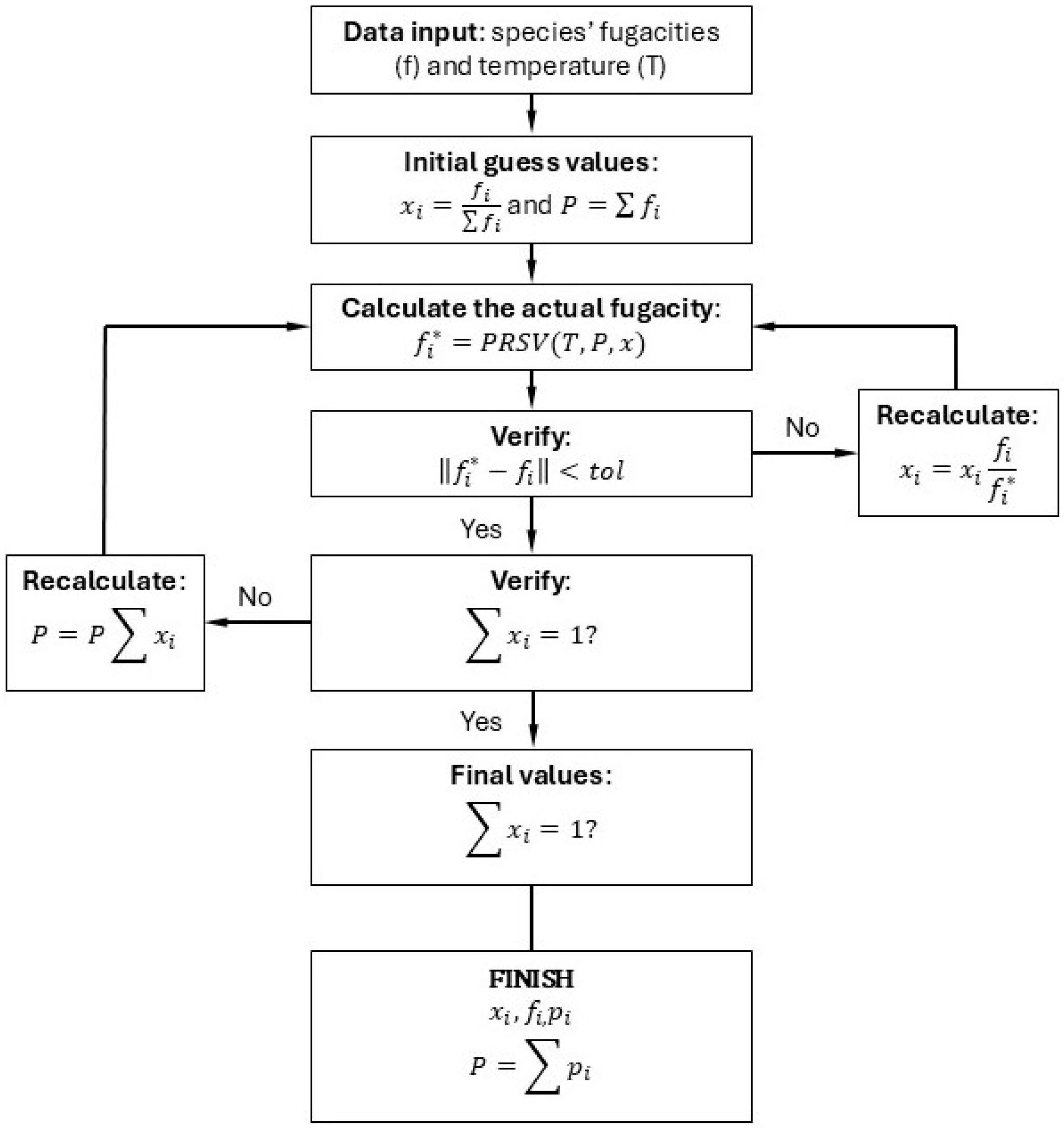
2.3. Thermodynamic Equilibrium in the Annulus

The species’ fugacity and pressure in the annulus increase with the permeation of the gases from the bore either in dry or flooded annulus conditions, implying a variation in the diffusivity and solubility coefficients with time, as can be perceived in Equations (8)–(12). Therefore, the fugacity and the pressure in the annulus should be updated considering its actual composition, requiring using an equation of state (EOS) to evaluate the thermodynamic equilibrium. This work assumes the Peng–Robinson–Stryjek–Vera (PRSV) EOS [25], as Appendix A describes.
The annulus pressure is calculated assuming that only gaseous substances are present. In such cases, the global system’s molar composition becomes the phase molar composition, and the algorithm shown in Figure 3 requires only species’ fugacities as input to estimate the molar composition and pressure. This algorithm is a back substitution to evaluate the fugacity through the PRSV equation until it matches the calculated annulus fugacity.

2.4. Heat Transfer in Flexible Pipes

The temperature significantly affects mass transport, so it is necessary to evaluate the pipe’s temperature profile to model the mass transport correctly. Fourier’s law describes the heat transport in stiff and isotropic materials under a temperature gradient [6]:
ρ   c s   T ˙ = k   2 T
where ρ , c s , and k are, respectively, the material’s density, specific heat, and thermal conductivity.
This work applies simplified hypotheses to simulate heat transport in flexible pipes, such as considering just heat transport by conduction and neglecting gaps in the annulus. Hence, Equation (8) is simplified to a one-dimensional cylindrical equation. Other hypotheses concern the stationary time of the phenomenon, i.e., while mass transport may take years to reach the permanent regime, heat transfer takes hours. Thus, the heat and mass transfer in flexible pipes are uncoupled phenomena, and Equation (8) can be reduced to the one-dimensional steady-state form:
1 r r   k r T r = 0
where r is the radial position of a point in a pipe layer.
This approach’s advantage is the possibility of solving Equation (16) analytically. The boundary conditions in Equation (16) are the bore’s fluid and seawater temperatures, assuming perfect contact between each layer. The method employed in this study is based on the work of Benjelloun-Dabaghi et al. [10], where further details can be obtained.
In the solution of Equation (16), the polymeric layers present a temperature gradient along their thicknesses due to the low thermal conductivity. At the same time, the steel armors exhibit a uniform temperature due to their high conductivity. The temperature has a direct impact on the materials’ diffusive properties. Nonetheless, a study conducted as part of this research [26] indicates that considering mean temperatures in the pipe’s polymeric layers leads to acceptable results compared to studies that evaluate the temperature gradient along the layer.

3. Numerical Model

3.1. Assumptions

This section describes the characteristics of permeation modeling in Ansys® software [14], divided into a primary section describing the main hypotheses and three other sub-sections referring to the modeling domain. The domain can be two- or three-dimensional. The two-dimensional model (2DFE) proposes an axisymmetric permeation domain, assuming the armor layers and intermediary tapes as rings. In contrast, the three-dimensional approach (3DFE) aims to detail the flexible pipe annulus space.
All models treat the mass transport problem through a fugacity reference, as it offers some advantages, such as the following:
  • Non-ideal representation of the species behavior, as discussed in Section 2;
  • Continuity in the annulus of the pipe, including at the layers’ interfaces. In contrast, the concentration of the species has a discontinuous distribution;
  • Better agreement with experimental measurements, according to Last et al. [10].
However, the model was developed in Ansys®, where no elements with fugacity as a degree of freedom are available. The software has specific finite elements to solve the mass transfer phenomenon, but it is developed in terms of concentration. Therefore, to avoid the development of a new finite element using fugacity as a degree of freedom, this work proposes an analogy between mass and heat transport.
Fourier’s law and Fick’s law are analogous parabolic equations, so it is possible to calibrate Fourier’s law parameters for amounting to Fick’s law. Therefore, this work assumes a thermal element with the temperature as the degree of freedom to evaluate the mass transport in fugacity reference. The analogy relies on the following:
  • Equaling temperature T and fugacity f ;
  • Equaling thermal conductivity k and permeability P e = S · D ;
  • Matching the specific heat capacity c s with the solubility coefficient S ;
  • Assuming density ρ as unitary.
Figure 4 indicates typical two- and three-dimensional FE meshes. The meshes are generated for the gaps between the discontinuous layers (tapes and armor layers) and the polymeric layers, which are assumed to be the porous medium. Their main characteristics are described next.

3.2. Two-Dimensional FE Model (2DFE)

The two-dimensional model (2DFE) employs an isoparametric element with one degree of freedom, temperature, at each node to describe the permeation domain (polymeric sheaths and annulus), as seen in Figure 4. This element, named PLANE177 in Ansys® [14], has eight nodes in its quadrangular shape (non-degenerated form) and considers three potential behavior possibilities: plane state, plane with thickness, and axisymmetric. Also, it has a quadratic interpolation. Moreover, the element requires three material properties, i.e., thermal conductivity, density, and specific heat, which are transformed to deal with the mass transport problem following the analogy described in the introduction of this section.
Calibration has been conducted to ensure equivalence between rings and layers in the case of modeling tapes and wires, which possess a helicoidal geometry. This equivalence ensures that the ring’s volume, surface area, and length are equivalent to the helicoidal geometry, similar to Benjelloun-Dabaghi et al. [10]. Equation (17) indicates the width s (Figure 5) of the space between two profiles:
s = 2 π R m tan φ n   w sin φ
where n is the number of wires or tapes, R m is the mean radius, w is the width profile, and, finally, φ is the laying angle.
Figure 4. Mesh and boundary conditions: (a) 2DFE model and (b) 3DFE model.
Jmse 12 02294 g004
Nevertheless, this equivalence is not straightforward for the pressure armor layers. Although all discontinuous layers (tapes and wires) are described as rectangular profiles, this assumption does not hold for the pressure armor, which usually has a Z cross-section (Figure 5). Hence, the intralayer gap length s is calculated through the wires’ width to ensure an equivalent shielding effect, as illustrated in Figure 5. This approach guarantees that the blocking surface over the pressure sheath is the same for both profiles.
Furthermore, one fundamental assumption in the modeling process pertains to the tapes, which can be classified as antiwear or anti-buckling. Unfortunately, the existing literature lacks information about the modeling of these tapes. Hence, this study proposes a hypothesis that considers the antiwear layers to be impermeable. This hypothesis assumes that the flux through the polymeric material can be neglected due to its low permeability. Therefore, the gas flows only through the gaps between the tapes. On the other hand, the anti-buckling tape, composed of aramid tissue, is intrinsically permeable due to its voids. Hence, this layer is treated as free volume, and a penalty factor is applied to simulate the actual free volume since gas cannot occupy spaces occupied by aramid.
Moreover, contact elements guarantee the interaction between layers, assuming no fugacity dissipation at the model’s interfaces (perfect contact). These contact elements are defined in pairs and are named CONTA174 and TARGE170 in Ansys®. In the proposed model, CONTA174 elements are placed on the annulus interfaces, while TARGE170 elements are placed on the opposite contact surface. If the contact is established between a polymeric sheath or a tape or armor layer, the CONTA174 elements are placed on the sheath surface, while TARGE170 elements are in the tape or armor layer interface.
The metallic layers and the polymeric tapes are admitted as impermeable (white regions in the two-dimensional model, Figure 4). Hence, following Benjelloun-Dabaghi et al. [10]’s remark, a “modeling” gap between the polymeric tape–armor layer interface was considered to avoid gas trapping, leading to an artificial pressure build-up. This gap was assumed to be 1% of the armor layer thickness in each interface and was modeled as an annulus region.
Regarding the boundary conditions, it is assumed that there is no mass flux through the ∂Ω borders (Figure 4). The inner surface of the pressure sheath is in phase equilibrium with the bore’s fluid, meaning that the fugacity of the bore’s fluid is equal to the absorbed gas fugacity on the pressure sheath. Conversely, the outer sheath is in equilibrium with seawater, which is admitted to flush out any gas escaping through the sheath, resulting in a fugacity equal to zero over the outer polymeric sheath’s external surface. Instead, the fugacity in the internal surface of the pressure sheath equals the fugacity of the gas in the bore. Additionally, equilibrium is maintained at each ∂Ψ interface between different layers, ensuring that the fugacity is equal on the contact regions.
The proposed model is suitable for both steady-state and transient analysis. However, in this work, only transient analyses were conducted. These analyses required a time step equivalent to 3 h to achieve suitable results. The FE meshes were constructed with a maximum element length of 0.5 mm, and a total length higher than 1.5 linear pitches of the pressure armor is sufficient to represent the phenomena.

3.3. Three-Dimensional FE Model (3DFE)

The three-dimensional model represents, in detail, the geometry of the pipe. Hence, isoparametric three-dimensional solid elements describe the permeation domain, as seen in Figure 4. This element is named SOLID238 in Ansys® and has 20 nodes in its hexahedral non-degenerated form and 10 nodes in a degenerated tetrahedral form, suitable to model irregular geometries.
Compared to the two-dimensional model, the actual modeling of the layers’ cross-section and lay angle makes the geometric equivalences and the interface gaps unnecessary. The detailed modeling of the cross-sections is achieved by using structured and unstructured FE meshes to capture the irregular geometry of the metallic layers and the annulus space. Moreover, the helical geometry of the tapes and the armor wires avoid trapping [13].
The contact between layers is established with the same contact elements employed in the two-dimensional model. However, the trustworthy representation of the three-dimensional domain increases the computational costs due to the layers’ detailed modeling and the necessity of many elements to couple continuous and discontinuous layers properly. In addition, Ansys® requires a minimal coincidence between contact surfaces to generate coupling equations, as establishing contact over the entire polymer and the wire surface would produce equations that link excessively distant nodes and produce incorrect results. The continuous layers are generated by rotating a plane around a Cartesian axis. In contrast, discontinuous layers are developed along the layer’s lay angle (Figure 6). Thus, achieving surface proximity between nodes from different layers requires high discretization, and the contact regions were discretized using elements having a maximum dimension of 0.2 mm after a few FE mesh tests. In all other areas, the same maximum element dimension assumed in the two-dimensional model was considered (0.5 mm). The length of the model should be higher than 1.5 linear pitches of the pressure armor.
Finally, the same time step as the 2DFE approach (3 h) was employed in the analyses with the three-dimensional model.

3.4. Implementation

The 2DFE and the 3DFE models are automatically generated with an APDL (Ansys Parametric Design Language) macro. Moreover, the macro controls the problem solution, updating the annulus diffusivity and solubility coefficients, relying on a user subroutine that calculates the annulus pressure with the algorithm presented in Figure 3 and Equations (8)–(10). Finally, the macro controls the solution of the problem, setting the sparse direct solver as the solution procedure.

4. Case Study

4.1. Description

A typical eight-layer 6″ flexible pipe layout was analyzed to evaluate the permeation phenomena. Table 1 describes its main characteristics. Despite an inner carcass in the pipe, this layer is not considered in the numerical analyses. The carcass profile allows fluid passage due to its interlocked cross-section, as seen in Figure 1. The fluid reaches the internal surface of the pressure sheath, and the imposed internal pressure typically opens a gap between the carcass and the pressure sheath [27]. Hence, a possible shield effect can also be conservatively neglected.
Furthermore, Table 2 presents the thermal conductivity in each layer and the Arrhenius parameters related to CO2 and CH4 for the PA11 and HDPE materials. The tapes and the metallic layers are assumed to be impermeable by hypothesis, as discussed in Section 2.2. The diffusivity and solubility of the annulus in dry and wet annulus conditions are calculated with the approach described in Section 2.2.1 and Section 2.2.2.
Finally, as the main objective of this work is to compare the two- and three-dimensional FE models’ responses when focusing on the SCC-CO2 phenomena, the following conditions were considered:
  • Internal and external temperatures of 60 °C and 5 °C, respectively;
  • Internal and external pressures of 500 bar and 200 bar, respectively;
  • CO2 and CH4 fugacities of 100 bar and 190 bar, respectively. These fugacities correspond to a bore composition of 60% CH4 and 40% CO2;
  • Both wet and dry conditions;
  • Total permeation analysis time of 2 years.
Next, a thermal analysis was conducted to determine the temperature in each layer, allowing the computation of the diffusive properties (diffusivity and solubility). Then, the permeation analyses’ results are presented and discussed.

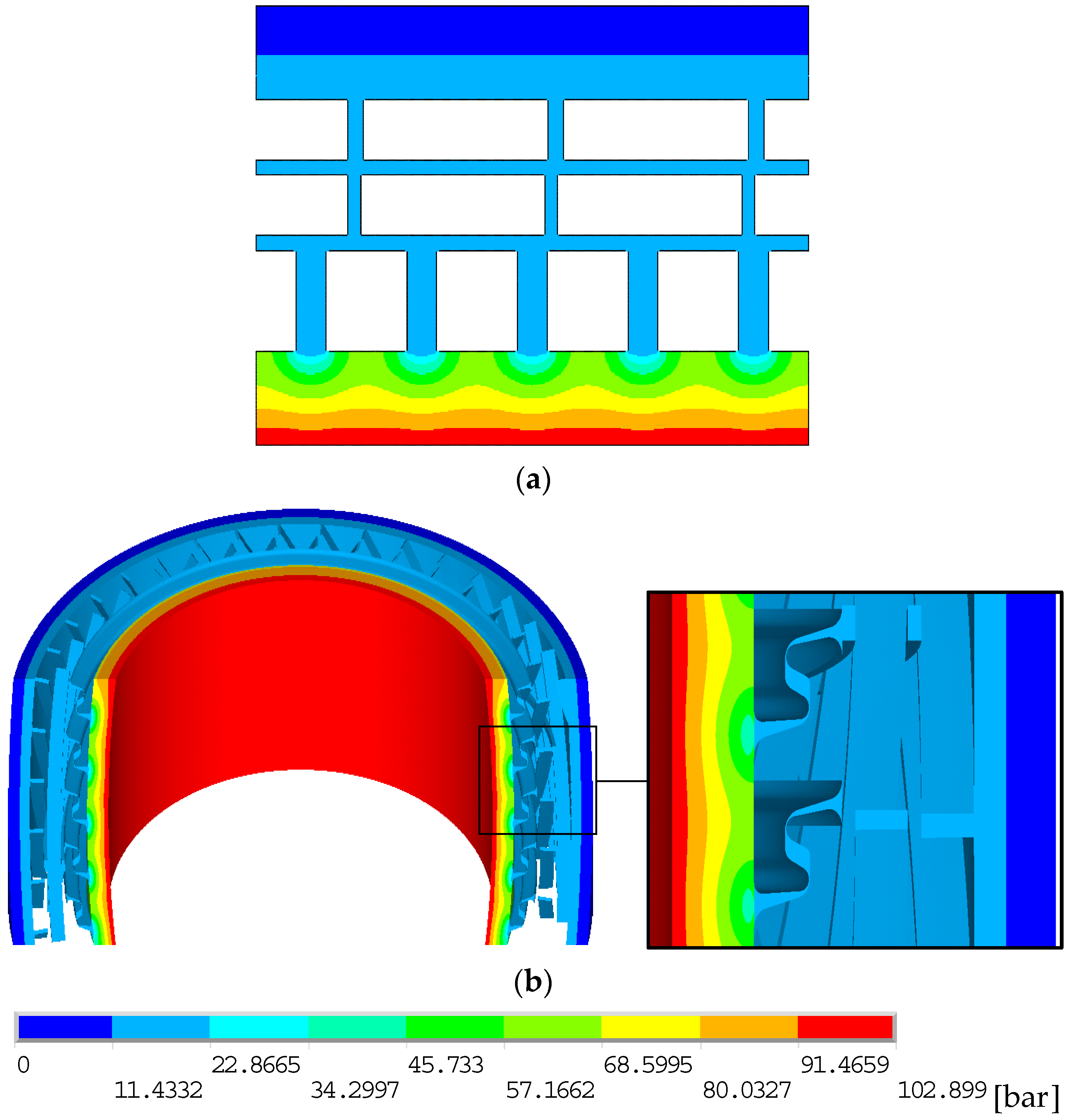
4.2. Thermal Analysis

The first step of a permeation analysis is to evaluate the thermal equilibrium through the material properties and the external and internal temperatures. Figure 7 shows the pipe’s temperature profile along the radial direction.
As expected, the analysis indicates that the polymeric sheaths are responsible for the pipe’s thermal insulation, while the metallic layers freely conduct the heat. The temperature linearly increases from 5 °C at the external surface of the outer sheath to about 23 °C at its internal surface. Analogously, a linear increase from 32 °C to the bore temperature (60 °C) is observed along the pressure sheath, evidencing the reasonable capacity of the sheaths to insulate the transported fluid. Moreover, it should be highlighted that these values are valid both for dry and wet annulus conditions, as pointed out in [26].
Once the temperature profile over the layers is evaluated, the diffusivity and the solubility of the CO2 and the CH4 in the permeation media are calculated with Equations (8)–(14) and Table 2. This work admits the mean temperature in each layer to obtain uniform permeabilities along the same layer.

4.3. Permeation Analyses

First, Figure 8 depicts the CO2 fugacity distribution across the pipe domain, demonstrating the homogeneous annulus fugacity distribution under dry annulus conditions after an operation time of 2 years. A similar distribution was obtained for CH4.
This uniformity arises from the high diffusivity in the annulus space, which offers no resistance to gas permeation. Consequently, when the fluid enters the annulus space, it fills all available volume. Therefore, as long as the structure remains sealed, the geometric effects occur only at the surfaces between a sheath and a discontinuous metallic sheath (pressure armor). The molecules become trapped beneath the impermeable profiles at these interfaces because the fluid cannot freely permeate through the polymeric matrix, resulting in the shielding effect (Figure 8). Thus, as the annulus internal geometry has minimal resistance and does not affect permeation, the 2DFE and 3DFE approaches are almost equivalent, as the annulus volume and the surface between the barrier and the metallic layer are equal in both models.
However, Figure 8 only qualitatively characterizes the approaches, highlighting the annulus scenario under a CO2 stationary flux regime and a dry condition. Subsequently, the models were separately evaluated to access the CO2 and CH4 fugacities’ variation over time, which are presented in Figure 9. This figure indicates that the two- and three-dimensional models agreed well, evidencing the significant potential of the two-dimensional model in accurately representing the permeation phenomenon in dry annulus conditions, in addition to considerably reducing the computational costs. The total time to simulate 2 years of operation was 20 min and 3 h for the 2DFE and 3DFE models, respectively. Moreover, the maximum CO2 fugacity is about 17.0 bar, while the maximum CH4 fugacity is 13.5 bar. These values correspond to 17% and 7% of the CO2 and CH4 fugacities in the bore and were reached after about 0.2 years and 0.6 years, respectively.
On the other hand, when the annulus is flooded, the water induces considerable resistance to the CO2 flow, and the annulus geometry plays a significant role in permeation. Hence, the annulus fugacity becomes non-homogeneous along the pipe length, presenting higher values close to the pressure sheath than in regions close to the outer sheath (Figure 10 and Figure 11). Observing only the 2DFE model, Figure 10 highlights some interesting permeation aspects. First, the geometric arrangement affects the annulus fugacity along the pipes’ length once the fugacity is low in locations with narrower escape paths. This effect results from the resistance induced by water that traps the molecules inside the complex annulus locations, allowing the molecules to flow only through the interconnected gaps, consequently reducing the fugacity in these zones.
Now, looking at the geometric aspects resulting from a three-dimensional analysis (Figure 11), other relevant effects arise. Figure 11 shows a significant difference in fugacity levels along the pipe’s circumference. Cross-section AA shows a fugacity profile that is different from the one in cross-section BB. This variation results from the non-axisymmetry of the free spaces, as the gaps between the wires are helicoidal in this model. Consequently, the molecules escape only at the intersection of these gaps.
Figure 12 depicts the contact between the inner tensile armor and the antiwear tape intralayer gaps. In the 3DFE model, the tapes are assumed to be impermeable, allowing molecules to only move from the tape gap to the tensile armor gaps. It is worth remarking that other layers are also impermeable, reducing the possible movement of molecules. In Figure 12, when the gas reaches the flooded gap of the antiwear tape, CO2 remains trapped until it can escape through the nearest opening, i.e., a contact region with a gap in the inner tensile armor. Hence, the diffusion restriction caused by water presence associated with the restrictions imposed by the impermeable layers results in high CO2 fugacities, which are reduced in regions where the molecules can freely permeate, as shown in Figure 12. This phenomenon is consistently observed at the interfaces of discontinuous layers, such as pressure and tensile armors and antiwear tapes. Finally, it is worth remarking that all these remarks regarding the flooded condition are also valid for the CH4 fugacity distribution.
Next, the CO2 and the CH4 annulus fugacities’ build-up were analyzed with the 2DFE and 3DFE approaches. As illustrated by Figure 10, Figure 11 and Figure 12, the annulus fugacity distribution is non-homogeneous. Hence, Figure 13 indicates the minimum and maximum CO2 and CH4 fugacities obtained with different approaches in SCC critical zones, i.e., in the pressure and inner tensile armors of the analyzed flexible pipe.
Comparing the 2DFE and 3DFE models, Figure 13 demonstrates that non-axisymmetry plays a critical role in predicting the composition of the annulus. In the 2DFE model, a “modeling” gap (represented as a continuous layer) is required at the interface between two discontinuous layers to prevent fluid trapping, allowing the gases to permeate freely from one discontinuous layer to another. On the other hand, in the 3DFE model, the fluid must find a connected gap (as shown in Figure 6 and Figure 12) to escape. Regarding the CO2, which is critical to the SCC mechanism in flexible pipes, these permeation characteristics result in maximum fugacity levels in the 3DFE model, being 2.7 and 1.8 times higher in the pressure and tensile armor spaces, respectively. Conversely, due to the continuous permeation path, the 2DFE model exhibits a higher minimum CO2 fugacity in the tensile armor. In contrast, the 3DFE approach has regions where molecules may become trapped or fail to occupy certain areas due to the dependence on the points of intersection between successive gaps. Hence, the 3DFE model shows higher maximum fugacities than the 2DFE model, where the CO2 may freely permeate. Analogous conclusions can be stated for the CH4.
Moreover, assessing the impact of a flooded annulus compared to a dry condition in the 2DFE and 3DFE approaches is crucial to the SCC-CO2 phenomenon. Therefore, Figure 14 illustrates the stationary CO2 fugacities along the radius of the pipe for the different proposed models and annulus conditions. However, as the geometry of the annulus induces a longitudinal gradient of the CO2 fugacity, this work proposes an envelope of fugacities. The envelope assumes the maximum and minimum fugacity values in each layer’s inner and outer radius. Through these results, a linear variation of the fugacity is considered in the layer.
Figure 14 shows that water significantly elevates CO2 levels within the annulus. In the pressure armor layer, the 3DFE model demonstrates a fugacity 6.1 times higher than the dry condition, while the 2DFE model indicates an increase of 4.2 times. Similarly, in the inner tensile armors, the 3DFE and 2DFE models exhibit CO2 levels 3.2 and 2.1 times higher, respectively, compared to the dry annulus. However, the dry annulus condition exhibited fugacity levels higher than the flooded condition in the top region due to the absence of resistance after passing the armors, making it easier for the gas to reach this region.
Additionally, when comparing the envelopes of the 2DFE and 3DFE models, Figure 14 indicates that the 3DFE model, constrained by its geometric limitations, increases fugacity levels throughout most radius sections of the pipes, except for the uppermost regions. The lower CO2 concentration in the upper region of the pipe can be attributed to the confined annulus geometry employed by the 3DFE model, which traps fluid in the lower annulus region, hindering CO2 from reaching the uppermost areas. However, the maximum fugacity value in the pressure sheath and the pressure armor obtained with the 3DFE model is close to the CO2 fugacity in the bore, while much lower values are predicted by the 2DFE model.
Nevertheless, as discussed in the dry annulus analyses, the 2DFE model requires much lower computational effort compared to the 3DFE model. Hence, a modified 2DFE model is proposed, aiming to approximate the maximum annulus fugacity values with those obtained with the most complex geometry represented in the 3DFE model.
A 2DFE analysis was conducted considering the same boundary conditions employed in the previously discussed flooded analysis but imposing the bore fugacities at the interface between the pressure sheath and the pressure armor, i.e., the diffusion through the pressure sheath was neglected. Figure 15 compares the 3DFE fugacity envelopes with those obtained with this modified 2DFE approach.
The results revealed that considering the bore’s fugacity in the pressure armor layers influences the 2DFE fugacity envelope, leading to a more conservative scenario across most of the free annulus space, except for the top of the pressure armor layer. These elevated values stem from the confinement geometry of the pressure armor’s Z profile in the 3DFE approach, which allows gas permeation only in specific zones, thereby increasing the fugacity levels in those trapping zones. Additionally, due to the confinement geometry, the 3DFE model consistently exhibits a significantly smaller minimum fugacity than the 2DFE model. This discrepancy arises because the continuous geometry of the 2DFE strategy facilitates a more uniform distribution of gas concentration, as shown in Figure 8. Nevertheless, apart from the higher levels at the top of the pressure armor layer, the 2DFE model, with the new boundary conditions, yields more conservative values in the more critical areas, the tensile armors. Specifically, the CO2 levels in the inner and outer tensile armors are 1.8 and 2.5 times higher in the 2DFE model compared to the 3DFE model.

5. Conclusions

This research aimed to develop and indicate numerical strategies for predicting the gas permeation from the bore into the flexible pipes’ annulus, focusing on CO2 permeation. Two FE models were developed that differ in the geometric domain. The first assumed an axisymmetric geometry of the annulus space, which reduced the three-dimensional domain to a two-dimensional domain, diminishing the number of degrees of freedom and the computational cost. On the other hand, a full three-dimensional model was admitted to evaluate the consequences of the geometry simplification.
Initially, both models underwent simulation and comparison under a dry annulus condition. The results obtained during this phase demonstrate a remarkable agreement between the 2DFE and 3DFE approaches. The fact that both models yielded similar annulus fugacity values underscores the negligible resistance offered by the dry condition to gas permeation, rendering the annulus geometry insignificant in this phenomenon. As a result, the study confirmed that the 2DFE approach is an excellent method for evaluating annulus composition under dry conditions, as its simplified geometry accurately represents the complete geometry without compromising precision while significantly reducing the computational time by approximately 115 times.
Sequentially, both models were evaluated and compared under a flooded annulus condition. The first observed consequence of a flooded annulus was the nonhomogeneity of fugacity values within the annulus. Consequently, at this stage, the fugacity results along the pipes’ radial axis were treated as an envelope of fugacities, which involved evaluating the maximum and minimum values within specific layer zones.
Therefore, the initial study compared the fugacity of a dry annulus under stationary conditions with the fugacity envelope obtained for a wet annulus condition. The findings revealed a significant increase in fugacity levels within the annulus. Specifically, the 2DFE exhibited 2.1 times higher fugacity under flooded conditions in the tensile armors’ region compared to the dry condition. Conversely, the 3DFE model demonstrated an even higher CO2 fugacity than the dry conditions, approximately 3.2 times higher. Hence, significant differences were observed between the 2DFE and the 3DFE models, making the 2DFE model less conservative.
Aiming to approximate the fugacities predicted by the 2DFE model to those evaluated in the 3DFE model under wet annulus conditions, a modified 2DFE model was constructed disregarding the pressure sheath. By doing that, the pressure armor’s fugacities equal the bore’s fugacity. The results obtained with this approach showed higher fugacities compared to the 3DFE model. Hence, this modified model may be an alternative to a more conservative design regarding SCC-CO2, demanding much lower computational effort.
Finally, this article dealt with different numerical approaches to predict flexible pipes’ annulus compositions during operation, assuming either dry or flooded conditions. However, several other aspects must be studied to adequately address crucial phenomena, such as SCC-CO2, e.g., the impact of the polymeric tapes in the diffusion phenomena; the presence of other acid gases and, more critically, water vapor in the diffusion process; the quantification of the corrosion phenomenon under different acid gases’ fugacities; and comparisons with experimental tests, which are critical to validate the proposed models.

Author Contributions

J.M.B.V.: Conceptualization, Methodology, Formal Analysis; Writing—original draft. J.R.M.d.S.: Conceptualization, Methodology, Supervision, Writing—review and editing. All authors have read and agreed to the published version of the manuscript.

Funding

The first author would like to acknowledge the financial support from ANP (the Brazilian National Agency for Petroleum, Natural Gas and Biofuels) implemented through its Program of Human Resources (code PRH 9.1), during his post-graduate studies at COPPE/UFRJ. Morover, this work was partially supported by the Brazilian funding agencies CNPq (Conselho Nacional de Desenvolvimento Científico e Tecnológico), grant number 308625/2022-6, and CAPES (Coordenação de Aperfeiçoamento de Pessoal de Nível Superior), finance code 001.

Data Availability Statement

The input and output data from the results of the analyses are available from the corresponding author upon reasonable request.

Conflicts of Interest

The authors declare no conflicts of interest.

Appendix A

Using cubic equations of state, such as the Peng–Robinson EOS, associated with the van der Waals mixing rule, is frequently employed to solve the problem of thermodynamic equilibrium in mixtures. However, this equation was used in this work but considering the modification proposed by Stryjek and Vera [25] (PRSV). The Peng–Robinson equation is given by:
p = R · T v b ¯ a ¯ v 2 + 2 · b ¯ · v b ¯ 2
where v is the molar volume of the system and a and b are parameters of the EOS. In a mixture, these parameters are obtained by combining the values of the pure components (van der Waals mixing rule):
a ¯ = i = 1 n f j = 1 n f x i · x j · a i , j
b ¯ = i = 1 n f x i · b i
where x is the molar fraction of each of the n f components in the mixture. In this work, n f equals 2 ( i , j = 1 to 2), as only CO2 and CH4 are considered. Moreover,
a i , j =           α i · p R · T 2 ,        i = j a i , i · a j , j · ( 1 k i , j ) ,        i j
α i = 0.457235 · R 2 · T C i 2 p C i · 1 + κ i · 1 T T C i 2
b i = β i · p R · T
β i = 0.077796 · R 2 · T C i 2 p C i
where p C and T C are the critical pressure and temperature of species i , and k is an interaction parameter, which, for the interaction between CO2 and CH4, equals 0.102. The parameter κ is given, according to Stryjek and Vera [25], by
κ i = κ i 0 + κ i 1 · 1 + T T C i · 0.7 T T C i
where κ i 0 equals 0.397 and 0.673 for CH4 and CO2, respectively, while κ i 1 is −0.0225 and −0.0679 for CH4 and CO2, in this order.
Equation (A1) may be written in the cubic polynomial form:
Z 3 ( 1 b ¯ ) Z 2 + ( a ¯ 2 b ¯ 3 b ¯ 2 ) Z ( a ¯ b ¯ b ¯ 2 b ¯ 3 ) = 0
where Z is the compressibility factor, which is stated as
Z = p · v R · T
Solving Equation (A1) by considering the parameters given by Equations (A2)–(A9), the compressibility factor Z is calculated. After that, the fugacity coefficient ϕ i may be obtained with
l n ϕ i = l n Z b ¯ + b i b ¯ · Z 1 a ¯ 2 2 b ¯ · 2 · j = 1 n f x i · a i , j a ¯ b i b ¯ · l n Z + 1 + 2 · b ¯ Z + 1 2 · b ¯
Finally, the fugacity of species i in the analyzed conditions is given by
f i = ϕ i · x i · P
where P is the system’s internal pressure.

References

  1. API. API RP 17B: Recommended Practice for Flexible Pipe, 6th ed.; American Petroleum Institute: Washington, DC, USA, 2024. [Google Scholar]
  2. Revie, R.W.; Uhlig, H.H. Corrosion and Corrosion Control: An Introduction to Corrosion Science and Engineering, 4th ed.; Wiley-Interscience: Hoboken, NJ, USA, 2008; pp. 150–166. [Google Scholar]
  3. ANP. Stress Corrosion Due to CO2 (SCC-CO2). Security Alert 001. Agência Nacional do Petróleo. 2017. Available online: https://www.gov.br/anp/pt-br/assuntos/exploracao-e-producao-de-oleo-e-gas/seguranca-operacional/incidentes/arquivos-alertas-de-seguranca/alerta-01/alerta-de-seguranca_001_ssm_scc-co2_pt.pdf (accessed on 19 November 2024). (In Portuguese)
  4. Fonseca, D.; Tagliari, M.R.; Guaglianoni, W.C.; Tamborim, S.M.; Borges, M.F. Carbon Dioxide Corrosion Mechanisms: Historical Development and Key Parameters of CO2-H2O Systems. Int. J. Corros. 2024, 2024, 5537767. [Google Scholar] [CrossRef]
  5. de Motte, R.; Joshi, G.; Chehuan, T.; Legent, R.; Kittel, J.; Désamais, N. CO2-SCC in Flexible Pipe Carbon Steel Armour Wires. Corrosion 2022, 78, 547–562. [Google Scholar] [CrossRef]
  6. Gurtin, M.E.; Fried, E.; Anand, L. The Mechanics and Thermodynamics of Continua; Cambridge University Press: Cambridge, UK, 2010. [Google Scholar]
  7. Eide, J.T.W.; Muren, J. Lifetime assessment of flexible pipes. In Proceedings of the ASME 2014 33rd International Conference on Offshore Mechanics and Arctic Engineering (OMAE2014), San Francisco, CA, USA, 8–13 June 2014. [Google Scholar]
  8. Eriksen, M.; Engelbreth, K.I. Outer cover damages on flexible pipes—Corrosion and integrity challenges. In Proceedings of the ASME 2014 33rd International Conference on Offshore Mechanics and Arctic Engineering (OMAE2014), San Francisco, CA, USA, 8–13 June 2014. [Google Scholar]
  9. Kristensen, A.B. Diffusion in Flexible Pipes. Master’s Dissertation, Technical University of Denmark, Lingby, Denmark, 2000. [Google Scholar]
  10. Benjelloun-Dabaghi, Z.; Hemptinne, J.-C.; Jarrin, J.; Leroy, J.-M.; Aubry, J.-C.; Saas, J.N.; Condat, C.T. MOLDITM: A Fluid Permeation Model to Calculate the Annulus Composition in Flexible Pipes. Oil Gas Sci. Technol. 2002, 57, 177–192. [Google Scholar]
  11. Taravel-Condat, C.; Guichard, M.; Martin, J. MOLDITM: A Fluid Permeation Model to Calculate the Annulus Composition in Flexible Pipes—Validation With Medium Scale Tests, Full Scale Tests and Field Cases. In Proceedings of the OMAE03 22nd International Conference on Offshore Mechanics and Arctic Engineering, Cancun, Mexico, 8–13 June 2003. [Google Scholar]
  12. Last, S.; Groves, S.; Rigaud, J.; Taravel-Condat, C.; Wedel-Heinen, J.; Clements, R.; Buchner, S. Comparison of Models to Predict the Annulus Conditions of Flexible Pipe. In Proceedings of the Offshore Technology Conference, Houston, TX, USA, 6–9 May 2002. [Google Scholar]
  13. Lefebvre, X.; Khvoenkova, N.; de Hemptinne, J.C.; Lefrançois, L.; Radenac, B.; Pignoc-Chicheportiche, S.; Plennevaux, C. Prediction of Flexible Pipe Annulus Composition by Numerical Modeling: Identification of Key Parameters. Sci. Technol. Energy Transit. 2022, 77, 1–11. [Google Scholar] [CrossRef]
  14. Ansys, Inc. Ansys® Mechanical APDL (Release 2023 R1); ANSYS, Inc.: Canonsburg, PA, USA, 2023. [Google Scholar]
  15. Frisch, H.L. Sorption and Transport of Penetrants in Glassy Polymers. Polym. Eng. Sci. 1980, 20, 2–13. [Google Scholar] [CrossRef]
  16. Prausnitz, J.M.; Poling, B.E.; O’Connell, J.P. Properties of Gases and Liquids, 5th ed.; McGraw-Hill Education: New York, NY, USA, 2001. [Google Scholar]
  17. Lewis, G.N.; Randal, M. Thermodynamics and the Free Energy of Chemical Substances, 1st ed.; McGraw-Hill Book Company: New York, NY, USA, 1923. [Google Scholar]
  18. Hemond, H.F.; Fechner, E.J. Chemical Fate and Transport in the Environment, 4th ed.; Elsevier: San Diego, CA, USA, 2022. [Google Scholar]
  19. Fuller, E.N.; Schettler, P.D.; Giddings, C.J. New method for prediction of binary gas-phase diffusion coefficients. Ind. Eng. Chem. 1966, 58, 19–27. [Google Scholar] [CrossRef]
  20. Chang, P.; Wilke, C.R. Some Measurements of Diffusion in Liquids. J. Phys. Chem. 1955, 59, 592–596. [Google Scholar] [CrossRef]
  21. Kontogeorgis, G.; Voutsas, E.; Yakoumis, I.; Tassios, D. An Equation of State for Associating Fluids. Ind. Eng. Chem. Res. 1996, 45, 4310–4318. [Google Scholar] [CrossRef]
  22. Diamond, L.W.; Akinfiev, N.N. Thermodynamic description of aqueous nonelectrolytes at infinite dilution over a wide range of state parameters. Geochim. Cosmochim. Acta 2003, 67, 613–629. [Google Scholar]
  23. Diamond, L.W.; Akinfiev, N.N. Solubility of CO2 in water from −1.5 to 100 °C and from 0.1 to 100 MPa: Evaluation of literature data and thermodynamic modeling. J. Chem. Thermodyn. 2003, 208, 265–290. [Google Scholar] [CrossRef]
  24. Flaconnèche, B.; Martin, J.; Klopffer, M.H. Permeability, Diffusion and Solubility of Gases in Polyethylene, Polyamide 11 and Poly (Vinylidene Fluoride). Oil Gas Sci. Technol. 2001, 56, 261–278. [Google Scholar] [CrossRef]
  25. Stryjek, R.; Vera, J. PRSV—An Improved Peng-Robinson Equation of State for Pure Compounds and Mixtures. Can. J. Chem. Eng. 1986, 64, 323–333. [Google Scholar] [CrossRef]
  26. Vieira, J.M.B. Numerical Models to Predict Gases Diffusion in the Annulus of Flexible Pipes. Master’s Dissertation, Federal University of Rio de Janeiro, Rio de Janeiro, Brazil, 2023. Available online: http://www.coc.ufrj.br/pt/dissertacoes-de-mestrado/661-2022-5/10176-joao-marcos-bastos-vieira-3 (accessed on 19 November 2023). (In Portuguese).
  27. de Sousa, J.R.M.; de Sousa, F.J.M.; de Siqueira, M.Q.; Sagrilo, L.V.S.; de Lemos, C.A.D. A Theoretical Approach to Predict the Fatigue Life of Flexible Pipes. J. Appl. Math. 2012, 2012, 983819. [Google Scholar] [CrossRef]
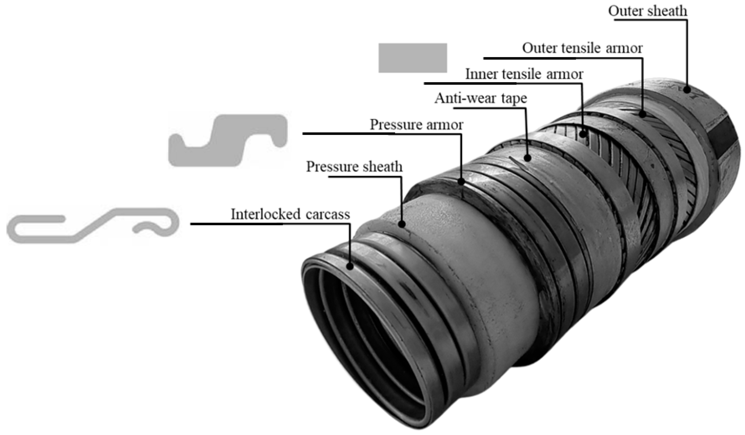
Figure 1. Unbonded flexible pipe.
Jmse 12 02294 g001
Figure 2. Comparison between capacity fugacity of CO2 in water from Kontogeorgis et al. [21], Diamond and Akinfiev [23], and experimental data [13].
Jmse 12 02294 g002
Figure 3. Algorithm to estimate the annulus pressure P.
Jmse 12 02294 g003
Figure 5. Equivalence for non-rectangular cross-sections.
Jmse 12 02294 g005
Figure 6. FE mesh in the interface between continuous and discontinuous layers.
Jmse 12 02294 g006
Figure 7. Radial temperature distribution in the analyzed 6″ flexible pipe.
Jmse 12 02294 g007
Figure 8. CO2 fugacity distribution in the annulus of the 6″ pipe with dry conditions after 2 years of operation: (a) 2DFE and (b) 3DFE.
Jmse 12 02294 g008
Figure 9. Fugacities’ build-up in the annulus space of the 6″ flexible pipe with dry conditions: (a) CO2 and (b) CH4.
Jmse 12 02294 g009
Figure 10. CO2 fugacity distribution in the annulus of the 6″ pipe with flooded conditions after 2 years of operation: 2DFE model.
Jmse 12 02294 g010
Figure 11. CO2 fugacity distribution in the annulus of the 6″ pipe with flooded conditions after 2 years of operation: 3DFE model.
Jmse 12 02294 g011
Figure 12. CO2 fugacity distribution in the gaps between the antiwear tape and the inner tensile armor of the 6″ pipe with flooded conditions after 2 years of operation.
Jmse 12 02294 g012
Figure 13. CO2 and CH4 fugacities’ build-up in the 6″ flexible pipe with flooded annulus conditions: (a) pressure armor, CO2; (b) inner tensile armor, CO2; (c) pressure armor, CH4; (d) inner tensile armor, CH4.
Jmse 12 02294 g013
Figure 14. CO2 fugacity envelopes considering dry and flooded annulus conditions: (a) 2DFE and (b) 3DFE.
Jmse 12 02294 g014
Figure 15. CO2 fugacity envelopes considering flooded annulus conditions: 2DFE with modified boundary conditions and 3DFE.
Jmse 12 02294 g015
Table 1. The 6″ (ID = 152.4 mm) flexible pipe characteristics.
No.Layer (Material)Properties
1Inner carcass 1
(stainless steel)
Thickness = 7.5 mm; Width = -; No of wires = 1;
Lay angle = 87.8°; intralayer gap, s = -
2Pressure sheath
(PA11)
Thickness = 9.3 mm
3Pressure armor
(carbon steel)
Thickness = 10.0 mm; Width = 10.5 mm; No. of wires = 2;
Lay angle = 87.6°; intralayer gap, s = 3.9 mm
4Antiwear tape
(polymeric tape)
Thickness = 1.5 mm; Width = 60.0 mm; No. of tapes = 1;
Lay angle = 79.7°; intralayer gap, s = 3.0 mm
5Inner tensile armor
(carbon steel)
Thickness = 6.0 mm; Width = 14.0 mm; No. of wires = 2;
Lay angle = 35.0°; intralayer gap, s = 1.3 mm
6Antiwear tape
(polymeric tape)
Thickness = 1.5 mm; Width = 60.0 mm; No. of tapes = 1;
Lay angle = 79.7°; intralayer gap, s = 3.0 mm
7Outer tensile armor
(carbon steel)
Thickness = 6.0 mm; Width = 14.0 mm; No. of wires = 2;
Lay angle = −35.0°; intralayer gap, s = 1.7 mm
8Anti-buckling tape
(aramid fiber)
Thickness = 2.3 mm
9Outer sheath (HDPE)Thickness = 9.3 mm
1 This layer is disregarded in the model, but the models maintain the ID of the pressure sheath. Hence, the width and the intralayer gap are not required.
Table 2. Thermal conduction coefficient, diffusivity, and solubility parameters for Arrhenius equations [24].
Material k
(W/mK)
Gas D 0
(cm2/s)
E D
(J/mol)
S 0
(cm3(STP)/cm3)
E S
(J/mol)
Stainless steel15.0CO2----
CH4----
Carbon steel45.0CO2----
CH4----
Polymeric tape0.24CO2----
CH4----
Aramid fiber0.20CO2----
CH4----
PA110.24CO20.4036,0005.40 × 10−3−12,000
CH44.5045,0007.50 × 10−20
HDPE0.54CO20.2032,0003.00 × 10−3−15,000
CH40.5036,0002.50 × 10−2−7000
Disclaimer/Publisher’s Note: The statements, opinions and data contained in all publications are solely those of the individual author(s) and contributor(s) and not of MDPI and/or the editor(s). MDPI and/or the editor(s) disclaim responsibility for any injury to people or property resulting from any ideas, methods, instructions or products referred to in the content.

