A LES-ALM Study for the Turbulence Characteristics of Wind Turbine Wake Under Different Roughness Lengths

Abstract

To investigate the characteristics of wind turbine wakes under different aerodynamic roughness lengths, a series of LES-ALM simulations were carried out in this study. First, a sensitivity analysis of the time step of the simulation results was performed. Then, the study compared the power and thrust of wind turbines under different roughness conditions. Finally, the mean velocity deficit, added turbulence intensity, and Reynolds shear stresses in the wake were analyzed under different roughness conditions. This study finds that a 0.1 s time step can provide satisfactory results for the LES-ALM compared to a 0.02 s time step. Furthermore, for the same hub-height wind speed, the thrust coefficient varies from 0.75 to 0.8 under the different roughness levels. As the roughness length increases, the time-averaged velocity deficit and added turbulence intensity decreases, and the wake recovers more quickly at the incoming level. However, the effect of roughness length on the Reynolds shear stress is weak within the downstream range of x = 6D to 10D. For the velocity deficit, a single Gaussian function is not able to describe its vertical distribution. Additionally, under higher roughness conditions, the height of the wake center is distinctively higher than the hub height as the wake develops downstream. The findings of this paper are beneficial for selecting the approximate numerical parameters for the wake simulations and provide deeper insights into the turbulence mechanisms of wind turbine wake, which are crucial for establishing analytical models to predict the wake field.

1. Introduction

1.1. Research Background

The Global Wind Report of 2023 claimed that, by the end of 2022, an additional 77.6 gigawatts (GW) of new wind power capacity had been successfully integrated into electrical grids across the globe [1]. This substantial increase brought the total global installed capacity of wind power to an impressive 906 GW. Along with this growth, the increase in wind farms and the enlargement of wind turbine sizes have led to smaller distances between wind turbines, intensifying mutual interference, known as the wake effects [2,3,4,5,6]. The airflow that drives the rotation of wind turbines converts part of its energy into the mechanical energy of the turbine’s rotation, creating a wake region characterized by reduced wind velocity and increased turbulence intensity. Figure 1 provides a schematic diagram of wind turbine wake. In wind farms, the wake can reduce the annual power generation by 10–20% [7]. Field measurement data from the Horns Rev wind farm show that the power output of the last row of turbines can be as low as 50–60% of the first row [8,9]. Furthermore, the presence of velocity deficits results in an added shear layer between the ambient flow and the wake, increasing turbulence intensity which will exacerbate the fatigue loads on downstream horizontal axis turbines [10,11,12] and vertical axis turbines [13,14]. The wake of wind turbines is strongly influenced by the inflow conditions which are controlled by roughness length and atmospheric stability [15,16,17,18,19,20]. Especially for some offshore wind turbines near the coast, the roughness lengths vary with wind direction. When the wind blows from the land, the roughness length is higher and the wind shear is stronger compared to when the wind blows from the sea. A detailed understanding of the turbulent features of wind turbine wake is essential for developing more accurate analytical models to predict the time-averaged velocity of a wake as well as the added turbulence intensity. This helps in calculating and analyzing the power output and fatigue loads of downstream turbines, optimizing onshore and offshore wind farm layouts, real-time control, and cost reduction, ultimately maximizing economic value.

1.2. Literature Review

Computational fluid dynamics (CFD) have been the primary tool for studying wind turbine wakes. In terms of turbulence model selection, compared to RANS methods such as k-epsilon and k-omega, LES can provide numerical simulation results that are more consistent with reality. Numerical simulations that fully model the actual shape of wind turbine blades require very fine mesh generation, leading to high computational demands and long modeling times, making them less frequently used. To address these challenges, alternative methods such as the actuator line method (ALM) have been developed [21,22,23]. This method simplifies the turbine blades into a line with aerodynamic force distribution along the radial direction, which is then applied to the body force term in the Navier–Stokes equations to simulate the interaction of the blades with the atmospheric boundary layer (ABL) wind field. Previous research has compared the effects of different grid resolutions [24,25,26,27], body force projection widths [28,29], and sub-grid stress coefficients [25] on wake characteristics. However, to simulate complex vortex structures induced by the blades, the time step may be strictly limited, ideally not exceeding the ratio of the grid size near the blade tip to the blade tip speed. In practical engineering, the space between wind turbines is typically 5–10D (D denotes the diameter of wind rotor), and the focus is often on the far wake characteristics rather than the near wake region. Therefore, it is necessary to compare the numerical simulation results of ALM under different time steps to provide more time-efficient parameter choices for wake simulations. This comparison can help optimize the trade-off between computational efficiency and simulation accuracy, ensuring that the simulations are both practical and informative for wind farm design and operation.

Full-scale wind turbine wake simulations better reflect the turbulent characteristics of the wake. While wind tunnel experiments can provide good wind turbine wake data, they suffer from inherent limitations due to the Reynolds number effects, making it difficult to fully reproduce full-scale wakes. Porté-Agel conducted relevant wind turbine wake experiments and found that the velocity distribution in the near wake is unimodal rather than the actual bimodal distribution [30,31]. This is mainly due to the inability of the wind turbine nacelle to scale accurately. Studies on the turbulent characteristics of wakes provide a data foundation for establishing wind turbine wake models. Early on, for ease of application in engineering, Jensen proposed the famous top-hat analytical model [32]. In Jensen’s work, it has been mentioned that the lateral profile of velocity deficit may better fit a Gaussian distribution. In 2014, Bastankhah and Porté-Agel raised the Gaussian wake model based on the Gaussian function [33]. Subsequently, Ishihara and Qian, Sun and Yang, Zhang et al., Tian et al., Ge et al. and others made corrections to the Gaussian model [34,35,36,37,38,39,40]. A Gaussian distribution is reasonable for the horizontal profile of velocity deficit because the boundaries of the wake can be assumed to be infinitely far. However, for the vertical distribution, a simple Gaussian distribution may produce some errors to predict the wake velocity deficit. Therefore, analyzing the lateral and vertical distribution characteristics of wake velocity deficit under different roughness length conditions through numerical simulations is of significant engineering importance.

As previously mentioned, the wake generates added turbulence intensity, significantly increasing the fatigue loads on wind turbines that are located in the wake region. The existing numerical simulations [22,26,41], wind tunnel experiments [34,42,43], and field measurements [44,45] observed enhanced turbulence intensity in the wake. These studies have revealed that the added turbulence intensity exhibits clear three-dimensional spatial distribution characteristics. Although some analytical models have been developed to predict added turbulence intensity, they often overlook the relationship between turbulence intensity and velocity deficit, leading to prediction inaccuracies [46,47,48]. Furthermore, in the layout of wind farms and the real-time control strategies of wind farms [49,50], the accurate prediction of added turbulence intensity is essential. This ensures that the fatigue loads on wind turbines within the wind farm are evenly distributed, thereby reducing maintenance costs and improving the overall efficiency and reliability of the wind farm. Roughness length not only affects the distribution and recovery of wake velocity deficits but also influences the spatial distribution characteristics of added turbulence intensity. Therefore, investigating its mechanisms and spatial distribution characteristics is also significant to calculate the fatigue loads of wind turbines and the maintenance costs of a wind farm.

1.3. Contributions of Paper

This paper uses a combined approach of ALM-LES to study and analyze wake characteristics under different roughness conditions. As mentioned earlier, there is a lack of investigation into the sensitivity of wake turbulence to time step using the ALM. Additionally, few studies systematically examine wake characteristics under different roughness lengths and analyze their added turbulence intensity and Reynolds stress levels. Therefore, the main contributions of this paper are: (1) This paper analyzes the thrust and power and the turbulent features of the wind turbine wake under the different time steps within the ABL flow. This analysis helps to understand the sensitivity of the simulation results to the choice of time step, which is crucial for optimizing computational efficiency while maintaining accuracy; (2) The study investigates how the thrust and power vary with changes in roughness lengths. This is important for designing wind turbines that can operate efficiently under different roughness lengths, including onshore and offshore conditions; (3) The paper explores the turbulent features of wakes and their spatial distribution properties under different roughness lengths. The simulation results provide insights into how roughness conditions affect the wake structure and turbulence, which is essential for optimizing wind farm layout and improving the overall performance of wind turbines.

The structure of the paper is as follows: Section 2 introduces the framework of LES and ALM. Section 3 presents the verification of time step independence and the reliability of the numerical simulation methods. Section 4 discusses the thrust and power of wind turbine as well as the wake turbulent characteristics, including mean velocity deficit, turbulence intensity and Reynolds shear stress. Finally, conclusions and summaries are provided.

2. Numerical Simulation Method

All numerical simulations are conducted on the SOWFA platform developed by NREL using OpenFOAM 2.4.X [15,51]. The LES is chosen as the turbulence model in this study, and the governing equations for LES and ALM will be provided in this section.

2.1. LES Framework

In order to simulate the wind flow, filtered incompressible Navier–Stokes Equations are solved to capture the resolved large-eddy scale flow feature, given as

$${\displaystyle \frac{\mathsf{\partial }{\overline{u}}_i}{\mathsf{\partial }{x}_i}}=0$$

(1)

where the overbar represents spatial filtering and ${\overline{u}}_i$ denotes the resolved-scale velocity vector. The filtered momentum Equation is

$$\underset{(1)}{\underbrace{{\displaystyle \frac{\mathsf{\partial }{\overline{u}}_i}{\mathsf{\partial }t}}}}+\underset{(2)}{\underbrace{{\displaystyle \frac{\mathsf{\partial }}{\mathsf{\partial }{x}_j}}({\overline{u}}_j{\overline{u}}_i)}}=\underset{(3)}{\underbrace{-2{\epsilon }_{i3k}{\mathrm{\Omega }}_3{\overline{u}}_k}}-\underset{(4)}{\underbrace{{\displaystyle \frac{\mathsf{\partial }\tilde{p}}{\mathsf{\partial }{x}_i}}}}-\underset{(5)}{\underbrace{{\displaystyle \frac{1}{{\rho }_0}}{\displaystyle \frac{\mathsf{\partial }}{\mathsf{\partial }{x}_i}}{\overline{p}}_0(x,y)}}-\underset{(6)}{\underbrace{{\displaystyle \frac{\mathsf{\partial }}{\mathsf{\partial }{x}_j}}({\tau }_{ij}^D)}}-\underset{(7)}{\underbrace{{\displaystyle \frac{gz}{{\rho }_0}}{\displaystyle \frac{\mathsf{\partial }}{\mathsf{\partial }{x}_i}}{\rho }_b}}+\underset{(8)}{\underbrace{{\displaystyle \frac{1}{{\rho }_0}}{f}_i^T}}$$

(2)

where Term 1 and Term 2 denote acceleration term and convective term, respectively; Term 3 represents the Coriolis force, which arises due to the Earth’s rotation; Term 4 describes the gradient of a modified pressure variable; Term 5 is the background driving pressure gradient; Term 6 represents the gradient of shear stress, which includes the viscous stress effects and sub-grid stress effects. Term 7 uses the Boussinesq approximation to compute the effects of density differences; Term 8 denotes the body force, namely the force calculated by the ALM.

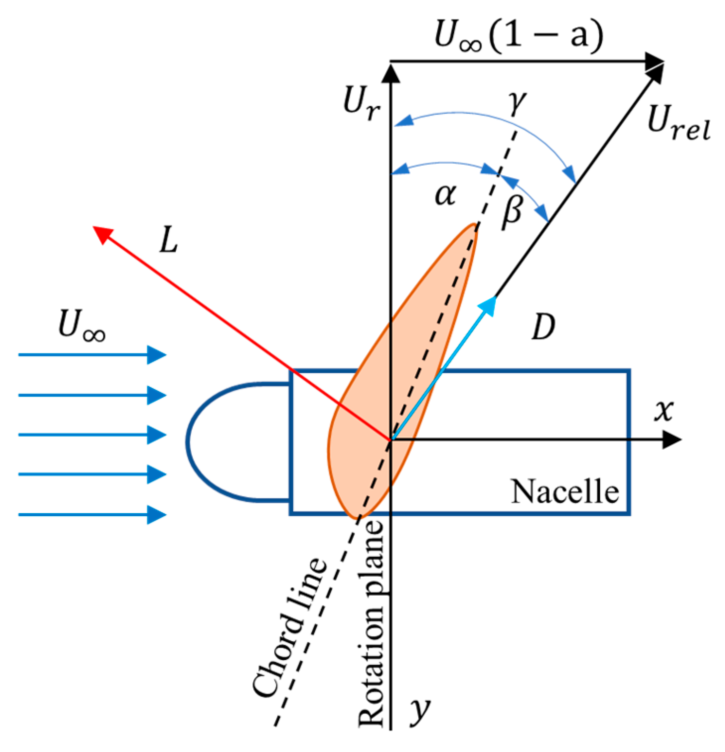
2.2. ALM Framework

This paper employs the ALM to calculate the forces induced by the wind rotor. To compute the aerodynamic force exerted on the turbine blades, we utilize the blade-element theory [52]. Figure 2 illustrates the relationship between wind velocity and the forces acting upon a blade element of a length $dr$.

Where $\alpha$ denotes the attack angle, $\beta$ represents the local pitch angle, $\gamma$ represents the angle between the resultant velocity and rotation plane. $d{F}_{\mathrm{L}}$ and $d{F}_{\mathrm{D}}$ denote the lift and drag forces, respectively, as follows

$$d{F}_{\mathrm{L}}={\displaystyle \frac{1}{2}}\rho U_{rel}^{2}c{C}_{\mathrm{L}}dr, d{F}_{\mathrm{D}}={\displaystyle \frac{1}{2}}\rho U_{rel}^{2}c{C}_{\mathrm{D}}dr$$

(3)

where $c$ represents the chord length, $C_{\mathrm{L}}$ and $C_{\mathrm{D}}$ denote lift and drag coefficient, respectively, $U_{rel}$ is the local resultant velocity, which is defined as $U_{rel}=\sqrt{U_{\infty }^2{(1-a)}^2+{(\mathrm{\Omega }r-U_r)}^2}$, where $U_{\infty }$ and $U_r$ denotes the inflow velocity and tangential velocity of the incident flow, $\mathrm{\Omega }$ is the rotating angular velocity of wind rotor.

At each location of blade element, a Gaussian distribution function is used to smooth the volume forces to multiple surrounding grid points

$$f={\displaystyle \frac{dF}{{\epsilon }^3{\pi }^{3/2}}}\exp {(-{\displaystyle \frac{r}{\epsilon }})}^2$$

(4)

where $\epsilon$ denotes a constant parameter of the Gaussian distribution, r denotes the distance between the mesh to the actuator point.

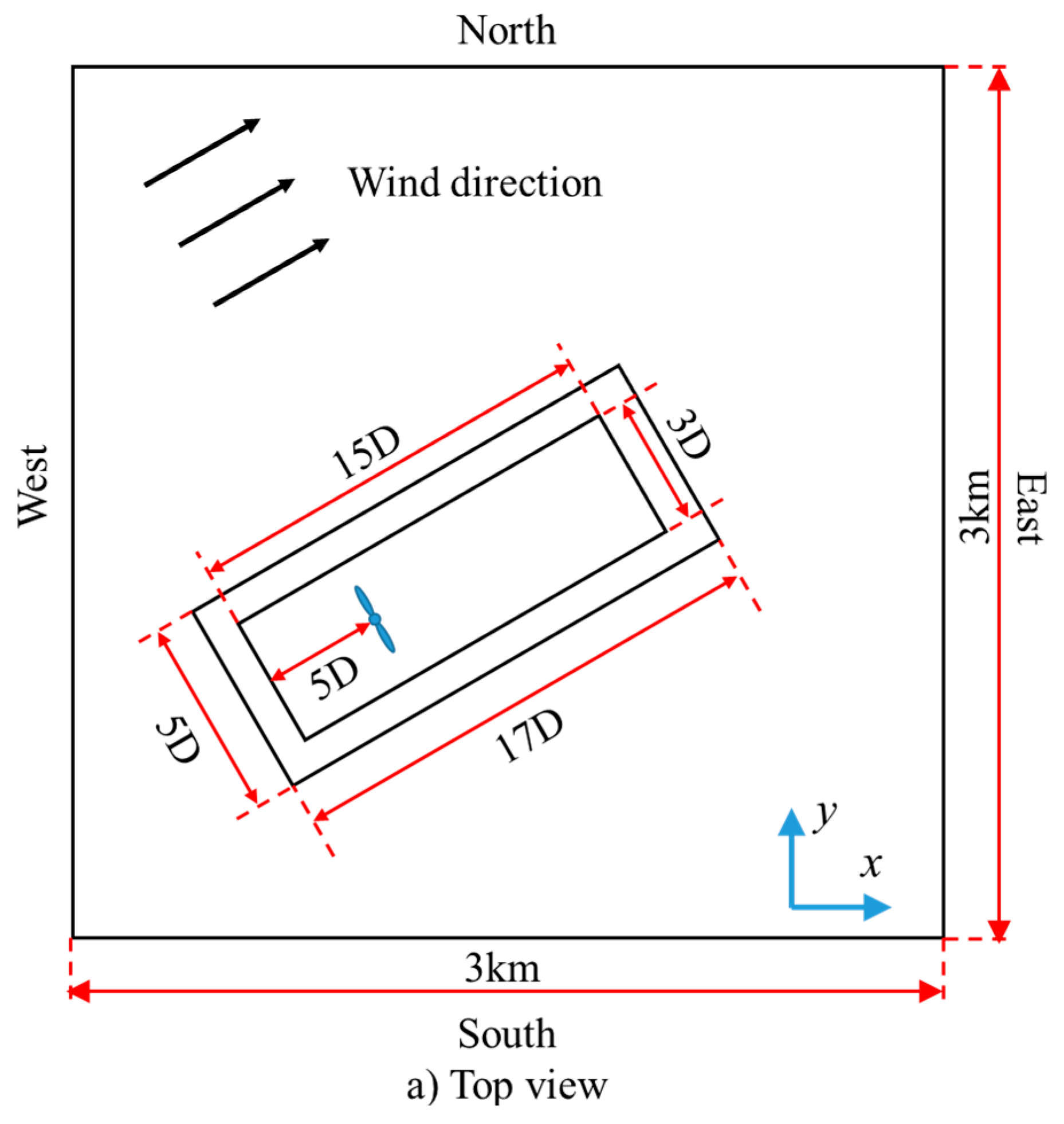
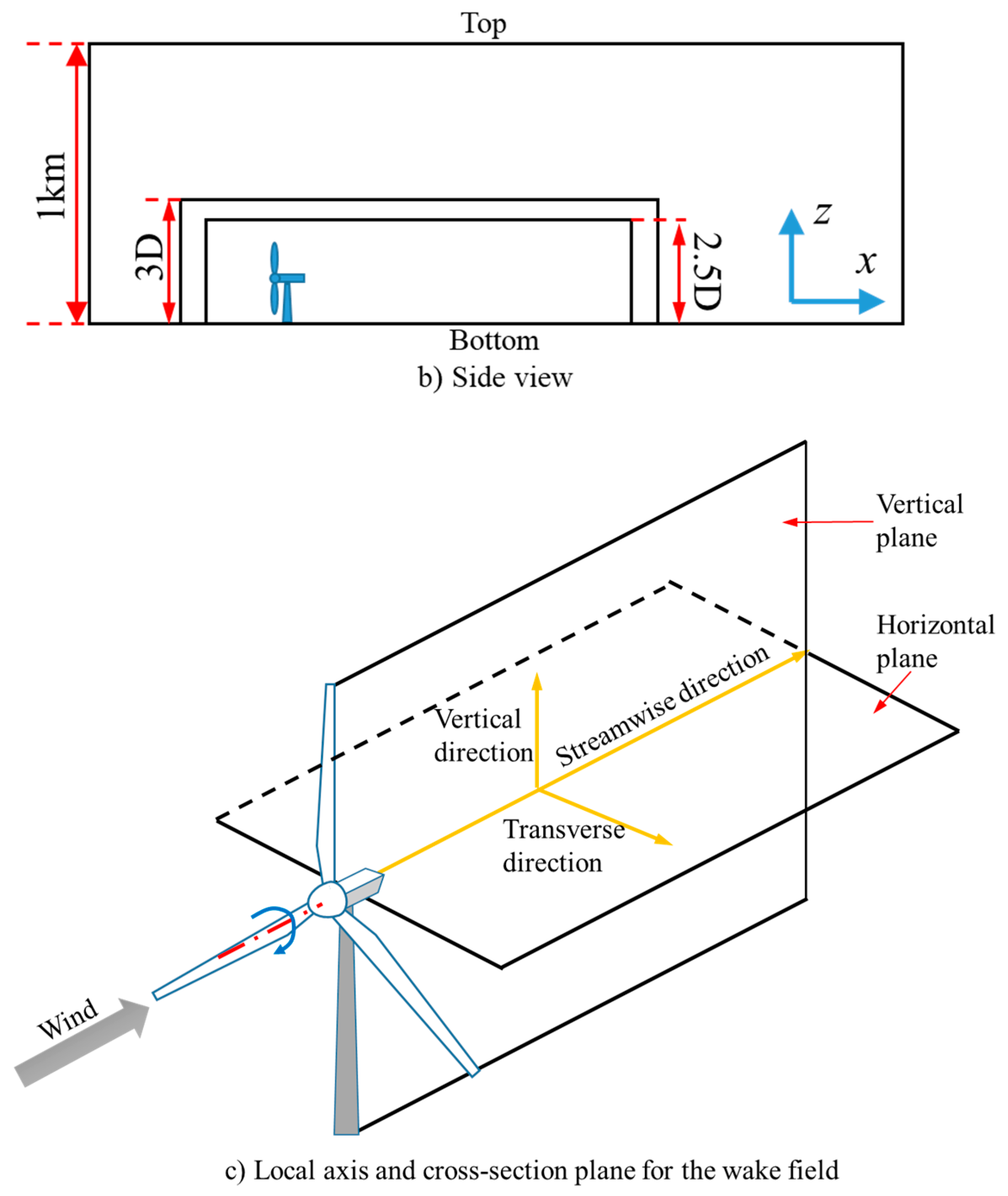
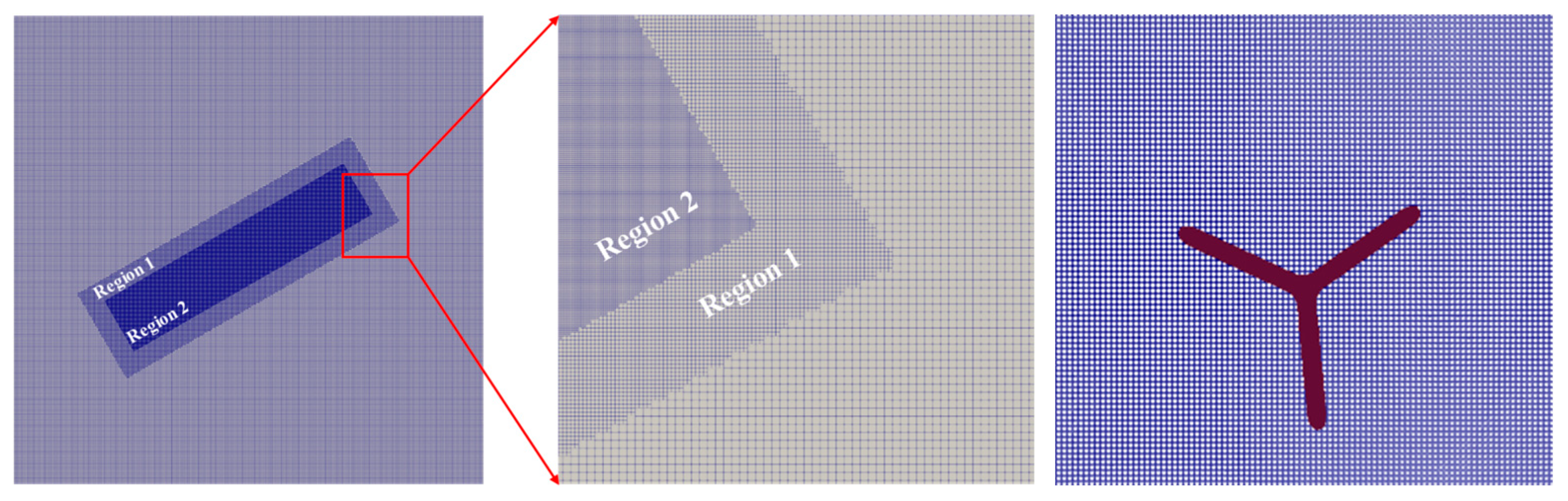
2.3. Domain Size and Mesh Distribution of Numerical Simulation

The accuracy of ABL simulations depends significantly on selecting a computational domain of sufficient size. Figure 3 provides a schematic diagram of the computational domain, as well as the local axis and cross-section plane for the wake field. Following the previous works [15,16,51,53], the numerical simulation domain size adopted in the present numerical simulation is 3 × 3 km horizontally and 1 km vertically. This domain size has been commonly selected for most relevant numerical simulations, and the size of wind turbines used in these simulations are similar, such as NREL 5 MW or Vestas V80-2 MW. Therefore, the discussion of the domain size will not be covered in this section. From Figure 3, the ABL direction is not parallel to the x-axis but rather forms an angle with it. This angle is fixed at 30 degrees. The cause for this selection is that if the inflow direction is parallel to the x-axis, i.e., parallel to the line connecting West and East, some very large turbulent structures would be fixed at certain crosswind positions (in the y-direction), which would not ensure a uniform distribution of mean wind speed at the same height [15,54].

Figure 4 provides a schematic picture of the grid generation for computational domain. For the ABL wind field, the computational domain is uniformly divided in three directions with a grid resolution of 10 m, which has $n_x\times n_y\times n_z=300\times 300\times 100$ grid cells. According to the guideline documents of SOWFA, the maximum grid resolution for ABL wind field is 20 m; therefore, the grid resolution used in this paper meets the requirements. When simulating the wind turbine wake to obtain more detailed information on the wake, local refinement is performed in the upstream region of the wind turbine, the wake region, and on both sides of the wind turbine. The grid resolution within Region 1 is 5 m and within Region 2 it is 2.5 m. The interval between the turbine model and the upstream boundary of Region 2 is 5D, and the distance to the downstream boundary of Region 2 is 10D. The transverse width of Region 2 is 1.5D. The vertical heights of Region 2 and Region 1 are 2D and 2.5D, respectively.

2.4. Numerical Parameters and Boundary Conditions of Simulation

The simulations process in this paper are primarily divided into two parts: the ABL wind field and the wake. The method used for simulating the ABL wind field is the precursor simulation approach. The precursor simulation approach involves conducting a separate simulation in a different computational domain before the wind turbine wake simulation, using periodic boundary conditions to simulate the ABL wind field. Firstly, an initial mean wind field is assigned to the numerical domain and then the numerical simulation is conducted to generate the turbulent fluctuations. Once the wind field reaches a steady state, instantaneous boundary data will be saved and adopted as the inlet condition for the wake numerical simulation. Moving forward, we will implement computational simulations to analyze the wake. The initial flow field is provided from the precursor simulation for ABL wind, with the previously saved boundary results serving as the inlet condition of wake simulation. The ALM is subsequently incorporated into the computational domain, after which the numerical simulation is executed. Figure 5 provides a flowchart of the numerical simulation process for this study.

The Reynolds numbers for atmospheric boundary layer flows typically range from 10⁶ to 10⁷, indicating that the boundary layer near the surface is very thin and almost impossible to resolve with a computational grid. To account for the effects of a rough surface on the ABL wind field, SOWFA incorporates the wall model based on the one proposed by Ref. [55]. This method can calculate the shear stress of the ground through the log law profile and the friction velocity. For the domain top, a slip boundary condition is employed. This boundary condition specifies that the normal velocity gradient of the boundary is equal to the normal gradient inside the computational cell adjacent to the boundary, while the normal velocity itself is zero. This ensures that there is a reasonable velocity gradient available when calculating the generation term for turbulent kinetic energy.

The streamwise ABL velocity at hub height, namely z = 90 m, is adopted as 8 m/s. The potential temperature is employed to be 300 K within the range from 0 m to 700 m, and it gradually raises to 308 K in the inversion layer ranging from 700 m to 800 m. The potential temperature gradient is 0.003 K/m at altitudes exceeding 800 m. The presence of the inversion layer beyond the top of ABL serves to dampen the increase in velocity with height during the simulation. The ABL wind field simulation is run for 18,000 s with a time step of 0.5 s and an adaptive maximum Courant number set to 0.75. After the wind field stabilizes, the data from the West and South boundaries between 18,000 and 21,000 s are saved to serve as the inlet boundary conditions for the wake simulation. In this part of numerical simulation, the time step is fixed at 0.1 s. During the wake numerical simulation, the first 500 s of data are discarded and not used for analysis, only the average flow field data for the last 2500 s are analyzed.

The characteristics of the ABL wind field are mainly controlled due to roughness lengths and atmospheric stability [42,56]. As the roughness increases, the wind shear within the ABL intensifies, further leading to increased turbulence. The turbulence intensity level significantly affects the turbulent features of the wake, such as the recovery rate of the wake and the distribution of velocity deficit and turbulence within the wake. Therefore, three different roughness length values are selected to compare the turbulent features of the wake under different terrain conditions.

Table 1. Specific roughness lengths adopted in the simulations [16].

Roughness Lengths z0 (m)	Roughness Category
0.00005	Calm sea
0.005	Short grasses (3 cm)
0.5	Long grass (60 cm), Crop

provides the specific surface roughness values used in the simulations along with their corresponding terrain types.

The NREL-5 MW wind turbine is a standard model designed by NREL in 2009, referencing existing conceptual wind turbine models and actual wind turbines at the time, as well as the minimum rated power that offshore wind turbines should have for a reasonable return on investment.

Table 2. Related parameters of NREL-5 MW.

Parameter Name	Parameter Values
Number of blades	3
Hub height	90 m
Diameter of wind rotor	126 m
Diameter of hub	3 m
Length of nacelle	6 m
Rotor tile angle	5°
Rotor cone angle	2.5°

provides some important parameters for the NREL-5 MW model. Under the rated condition, the corresponding rated rotational speed is 12.1 rpm. In this study, we adopt a rotor rotational speed of 9.1552 rpm, corresponding to the hub-height wind speed. TSR is 7.55 according to the inflow conditions and rotational speed. Table 2 lists the relevant parameters of the NREL-5 MW wind turbine.

3. Validation of Numerical Simulation Method

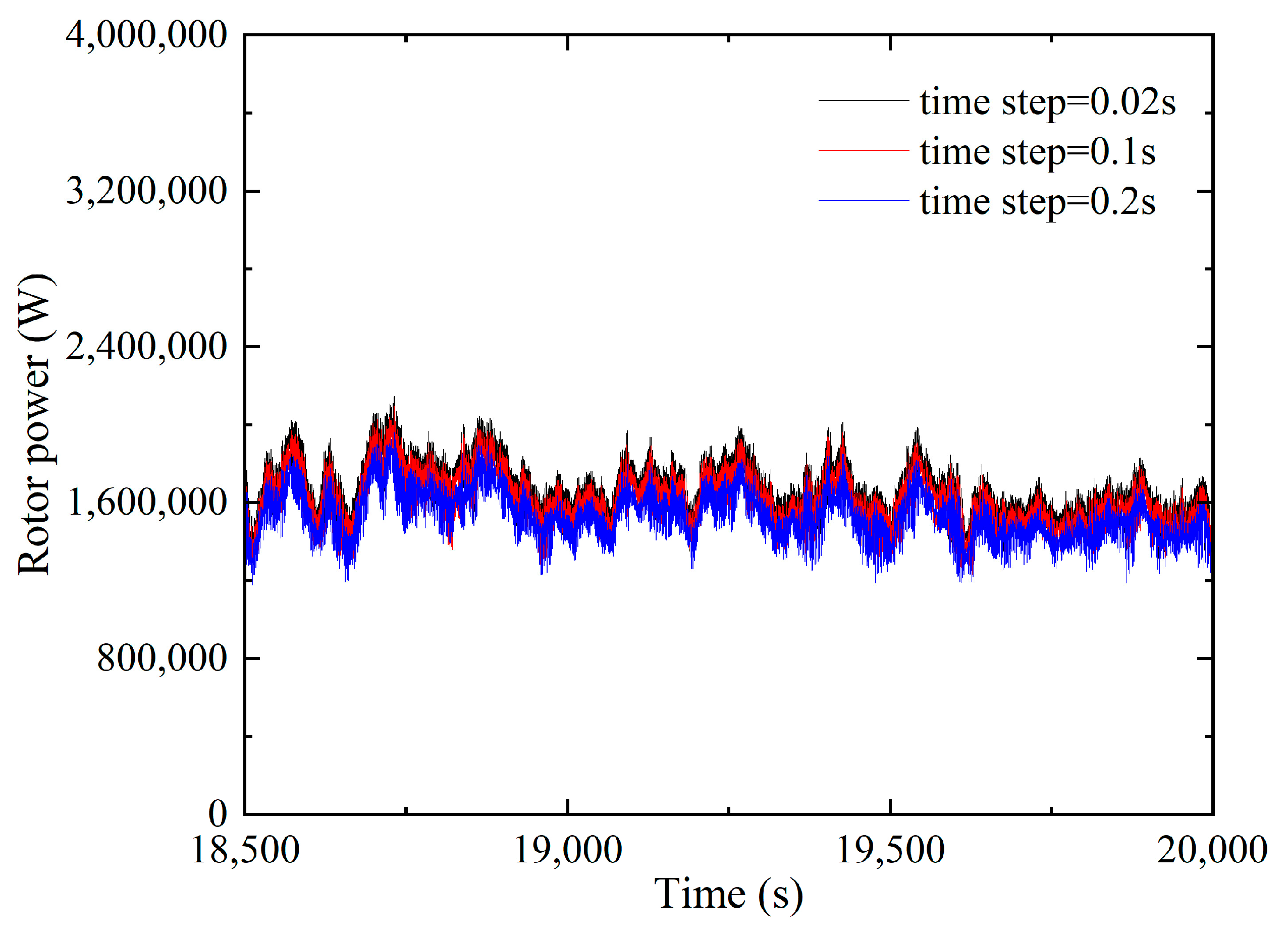
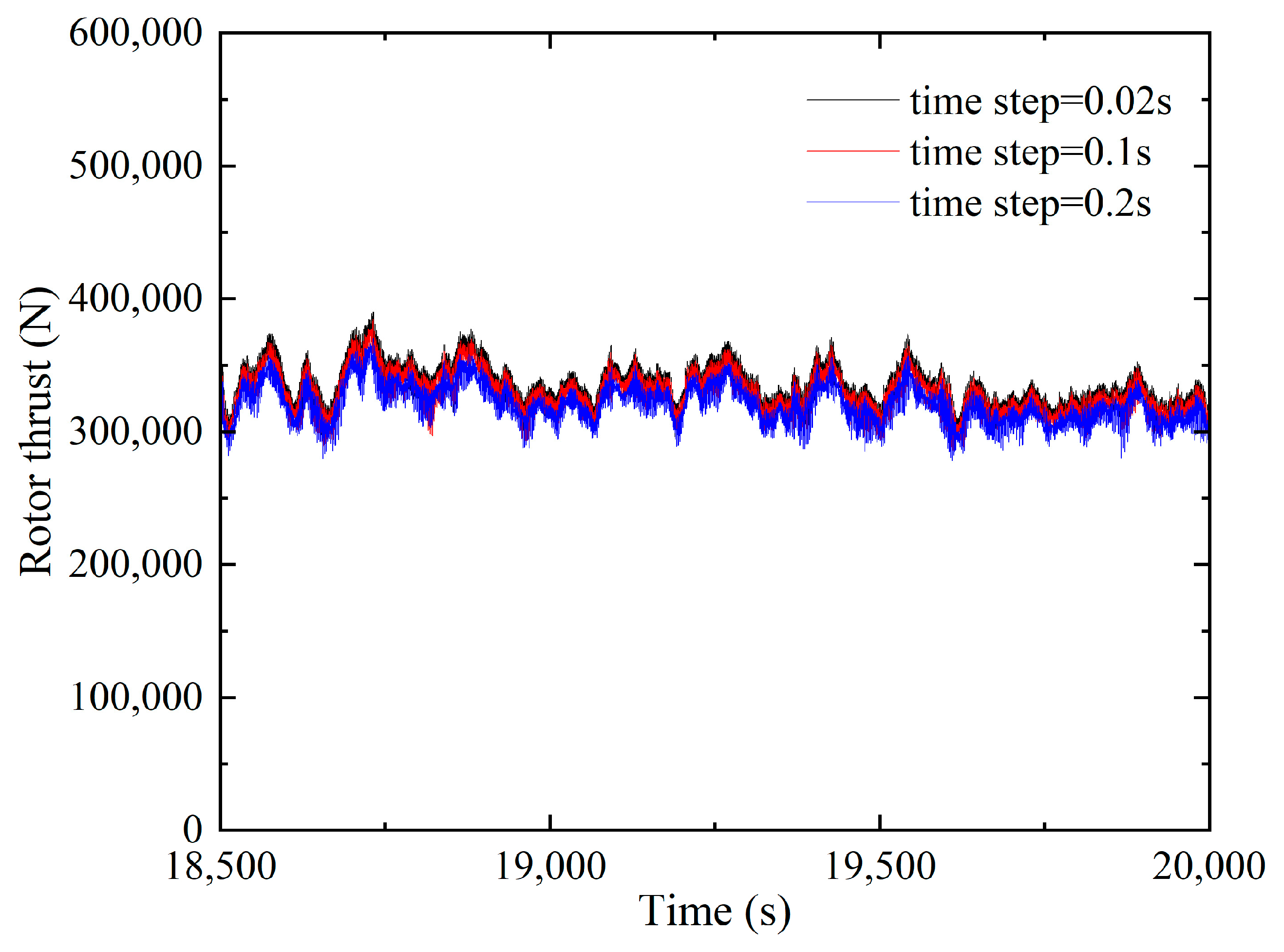
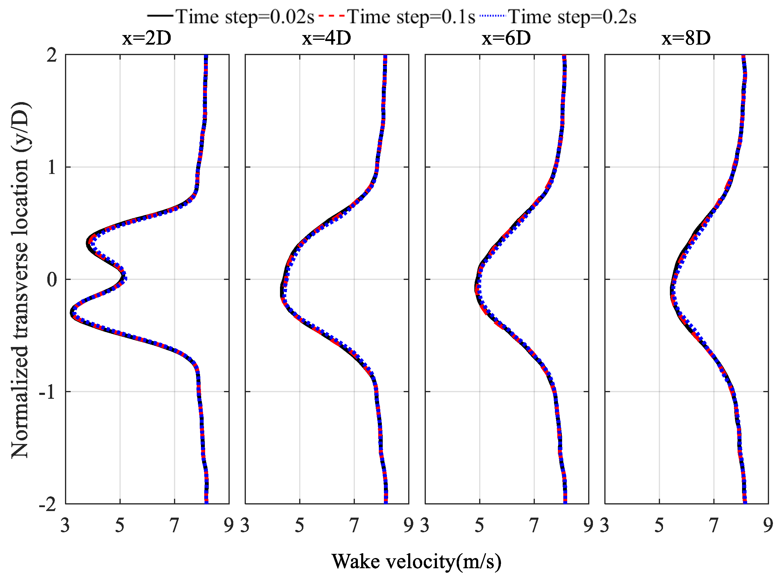
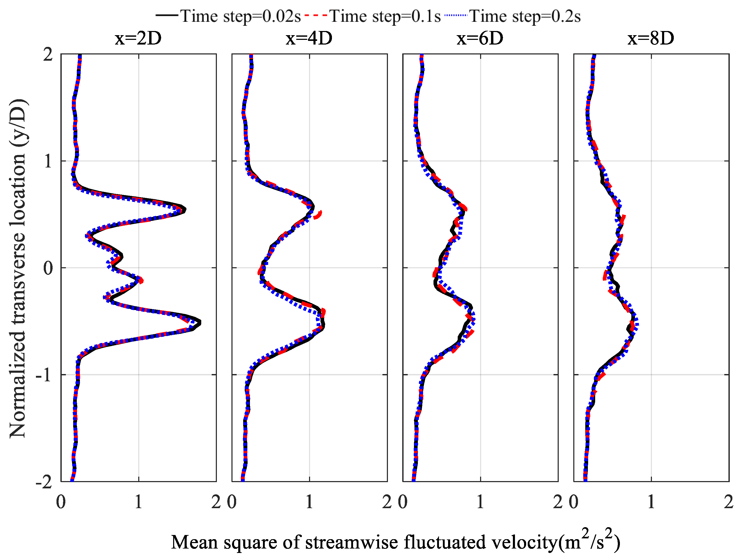
3.1. Independence Verification of Time Step

Typically, to simulate the tip vortices produced by the ALM, the time step selection does not exceed the ratio of the tip grid size to the speed of blade tip [15,22,57,58]. However, if the above standard is used to set the time step for LES-ALM, even when using the ALM to represent the actual blades of wind turbine, it would require a significant amount of simulation time. This paper focuses on the statistical properties rather than the vortex structures, and thus proposes using a larger time step for the numerical simulation. Therefore, the independence comparison is needed to validate the power and thrust of the wind rotor and turbulent characteristics of the wake field at different time steps.

Figure 6 shows the fluctuations of power over time. It is seen in Figure 6 that, across all time step cases, the wind turbine power fluctuates around 1,600,000 watts, namely 1.6 megawatts (MW). Comparing the power time histories reveals that the longer the time step, the higher the wind turbine power. However, the overall amplitude of the power fluctuations is similar across different time steps. To better evaluate the mean power under the different time steps, the value of 0.02 s time step is taken as a baseline, and the relative errors of mean power of 0.1 s and 0.2 s are calculated.

Table 3. Mean power and relative errors of the wind turbine under the different time steps.

Time Step (s)	Mean Power (W)	Relative Error
0.02	1,659,823.50	0%
0.1	1,612,428.92	2.9%
0.2	1,534,145.78	7.6%

provides the mean power and relative errors at the different time steps. The table reveals that the mean power decreases with increasing time step. When the time step is 0.1 s, the relative error is only 2.9%; however, when the time step is 0.2 s, the error reaches 7.6%. Through the comparisons, it can be concluded that the error under the time step of 0.1 s is acceptable.

Figure 7 illustrates the time histories of the fluctuating thrust of the wind rotor. Similarly to the case of power, as the time step increases, the mean thrust will decrease.

Table 4. Mean power and relative errors of the wind turbine.

Time Step (s)	Mean Thrust (N)	Relative Error
0.02	334,015.21	0%
0.1	329,200.93	1.4%
0.2	321,092.86	3.9%

shows that the mean thrust and relative errors for different time steps. The baseline is taken as the mean thrust at a time step of 0.02 s. The relative errors of the average thrust at 0.1 s and 0.2 s are calculated based on this baseline. The analysis reveals that with a time step of 0.1 s, the relative error amounts to 1.4%. However, when the time step is increased to 0.2 s, the relative error escalates significantly to 3.9%. This demonstrates a clear correlation between the size of the time step and the relative error value. In summary, with a time step of 0.1 s, the relative errors for both the average thrust and power compared to a time step of 0.02 s are small, and the accuracy is acceptable for the purposes of this study.

In this study, we are more concerned with the turbulent characteristics of wakes. Figure 8 presents the comparisons of the wake velocity at different time steps. We compare the hub-height wake velocities for four different downstream locations. From this figure, we can observe that regardless of whether within the near-wake region (x = 2D) or the far-wake region (x = 4D, 6D and 8D), the choice of time step does not have a significant impact on the profiles of mean wake velocity. This indicates that the time step independence exists for the mean velocity profiles within the wake region, which is important for the focus of this study on the turbulent characteristics of wind turbines wake.

Figure 9 presents comparisons of the squared streamwise fluctuating velocities within the wake under the different time steps. From Figure 9, we can obtain that, similarly to the mean wake velocity, the choice of time step does not have a significant impact on the squared streamwise fluctuating velocities. This indicates that the time step independence is also maintained for the fluctuating velocities within the wake region.

In summary, we have conducted a time step independence verification for four physical quantities: wind turbine power, wind turbine thrust, mean wake velocity, and squared streamwise fluctuating velocities in the wake. Based on the comparison of numerical simulation results at three different time steps, we find that selecting a time step of 0.1 s has little impact on the computational results. Therefore, for the remaining wake simulations in this paper, we will use a time step of 0.1 s.

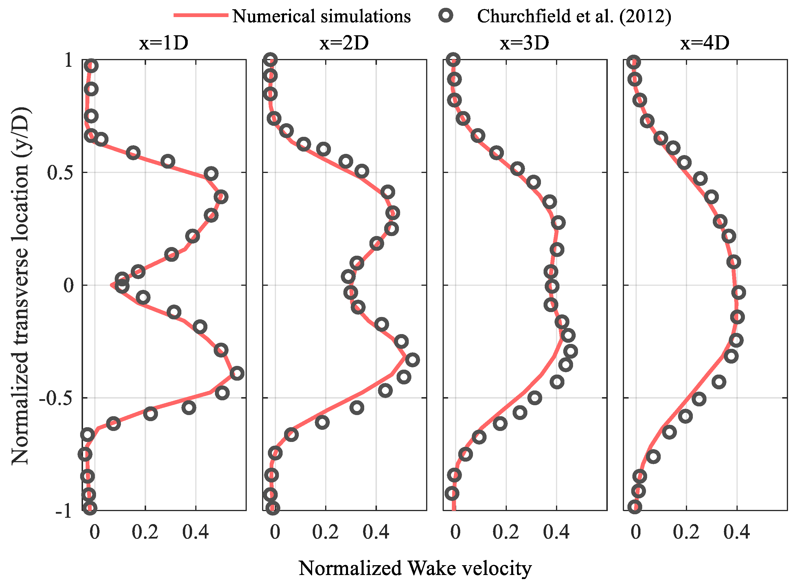
3.2. Validation of LES-ALM

Next, we will compare the numerical simulation results at a time step of 0.1 s with the results from Ref. [15] to validate the effectiveness of the numerical simulation methodology.

Table 5. Comparisons of the inflow turbulence intensity between the present simulation and the existing study.

	Churchfield et al. [15]	Present Simulations	Relative Error
$I_{\mathrm{bot}}$ (%)	5.9	5.8	1.7%
$I_{hub}$ (%)	4.9	5.0	2%
$I_{top}$ (%)	4.4	4.6	4.5%

provides the turbulence intensity at different heights for the incoming flow conditions. From the information in the table, it is evident that the incoming flow turbulence intensity simulated in this paper is consistent with the results from [15]. The maximum relative error occurs at the hub top, but it does not exceed 4.5%. Overall, the predicted results demonstrate good performance.

Figure 10 presents a comparison of dimensionless transverse velocity deficit profiles. The literature simulation focused on the double wind turbine wake, so the comparison is made with the upstream turbine wake information. This figure includes the velocity deficits at downstream 1D, 2D, 3D, and 4D. It can be observed that the simulation results are consistent with the results adapted from Ref. [13]. Hence, we argue that the numerical method used in this paper is reliable.

4. Numerical Results of LES-ALM

4.1. ABL Wind Field

The numerical simulation of the ABL wind is crucial for the simulation of the wake. The wind fields generated using the precursor simulation method exhibit good self-preservation, meaning that the turbulence statistics do not decay as they propagate downstream. Figure 11a shows the wind speed profiles of ABL under different roughness length. It can be observed that with increasing roughness length, the wind shear becomes more pronounced. Furthermore, all plots reach the pre-set hub-height wind speed of 8 m/s. Figure 11b presents the numerical simulation results for the streamwise turbulence intensity. Generally, the turbulence intensity decreases with increasing height. However, there is a maximum value around a height of 0.15 D from the ground. As roughness length increases, the streamwise turbulence intensity values also increase, indicating that the ABL wind becomes more turbulent.

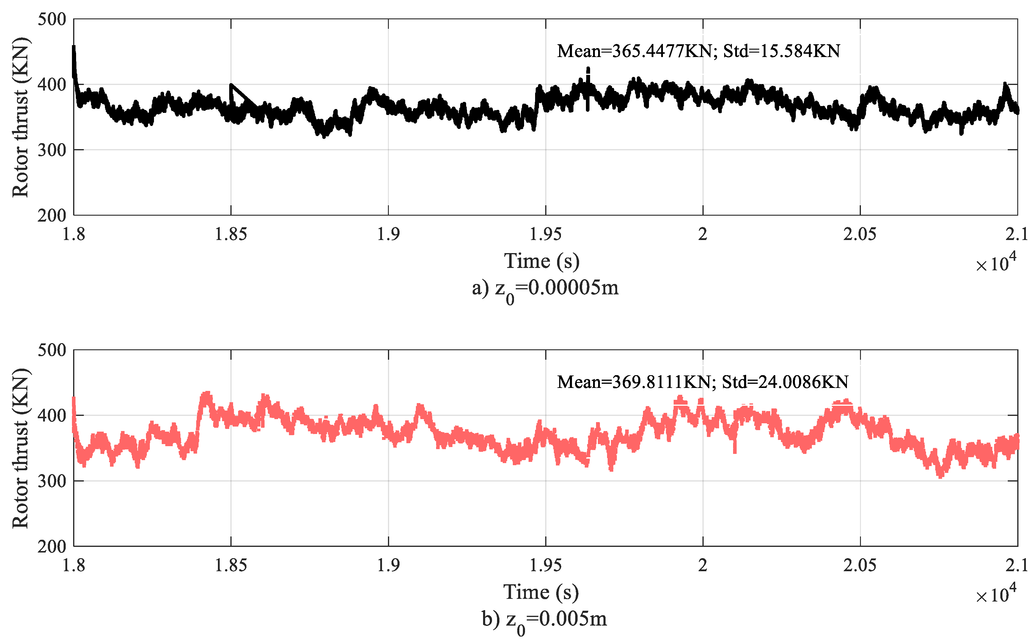
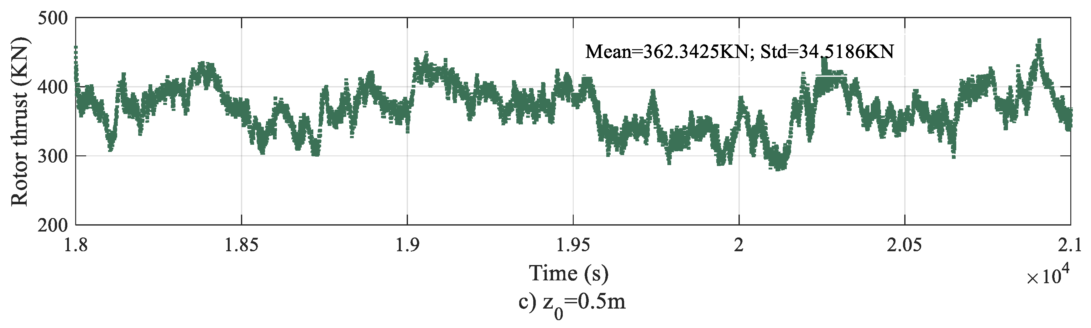
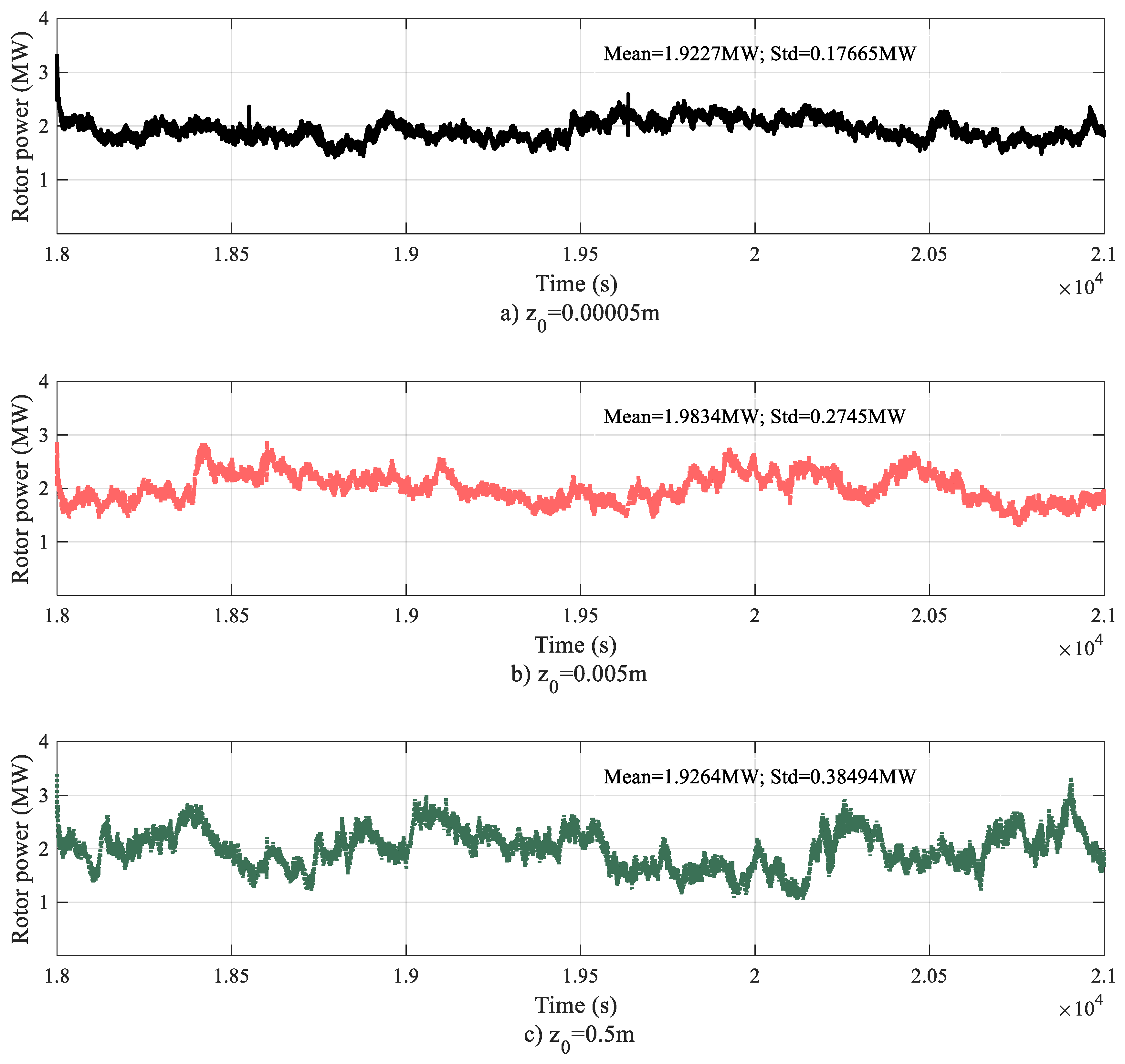
4.2. Mean Thrust and Power of Wind Rotor

Figure 12 provides the time histories for thrust and power under the different roughness length. In this figure, Mean represents the time-averaged value, and Std represents the standard deviation. Although previous researchers have conducted some studies on wake characteristics under the ABL wind, they have rarely compared the time histories, mean values, and standard deviations of wind turbine thrust and power under the different roughness lengths. In Figure 12, the wind turbine thrust will fluctuate over time. When the roughness length is 0.00005 m, the range of these fluctuations is generally between 320 KN and 400 KN. However, as the roughness length increases, the amplitude of these fluctuations gradually becomes larger. At 0.005 m, the fluctuation amplitude ranges from 300 KN to 420 KN. Under the condition of 0.5 m, the fluctuation range is the largest, reaching from 290 KN to 450 KN. We can see that under these three terrain conditions, the mean value of thrust is relatively close, around 365 KN. However, comparing the standard deviation of thrust reveals that the greater the roughness length, the larger the fluctuations in the wind turbine thrust, and thus the higher the standard deviation.

Figure 13 illustrates the curve of wind turbine thrust varying with time. Similarly to the thrust time series curve, the pulsation degree of power increases as the roughness length increases. Additionally, through calculations, the thrust coefficient under different roughness length conditions has been obtained. As mentioned above, the numerical simulations are set with same hub-height wind speed. However, it is found through calculations that the thrust coefficient and the thrust of wind differ under different roughness length conditions. The formula for calculating the thrust contained within the incoming wind here is:

$$\mathrm{Thrust} \mathrm{of} \mathrm{wind} ={\displaystyle \underset{A_D}{\iint }\frac{1}{2}\rho U^2\left(z\right)}dydz$$

(5)

When the roughness length is 0.00005 m, the thrust is the highest, with a corresponding $C_T$ of 0.75. At 0.005 m roughness length, the thrust coefficient is the highest, reaching 0.8. The values at 0.5 m and 0.00005 m have little difference, which are 0.76 and 0.75, respectively. Analyzing the thrust coefficient under different roughness length conditions is very meaningful. This will help us further analyze the wake velocity deficit under different roughness length conditions.

Figure 14 provides the time histories of power under different roughness length conditions. Similarly to the situation with wind turbine thrust, the pulsation degree of the power increases as the roughness length increases. When the roughness length is 0.00005 m, the pulsation curve of the power fluctuates within the range of 1.5 MW to 2.5 MW. Then, at the maximum roughness length, the range of pulsation fluctuations expands to between 1 MW and 3 MW. We also observe that the wind turbine power is greatest under the roughness length of 0.005 m, reaching approximately 1.98 MW. By comparing the standard deviations, we find that as roughness length increases, the fluctuation amplitude of the wind turbine power also grows larger. This indicates that the boundary layer turbulence significantly affects the fluctuations in wind turbine power.

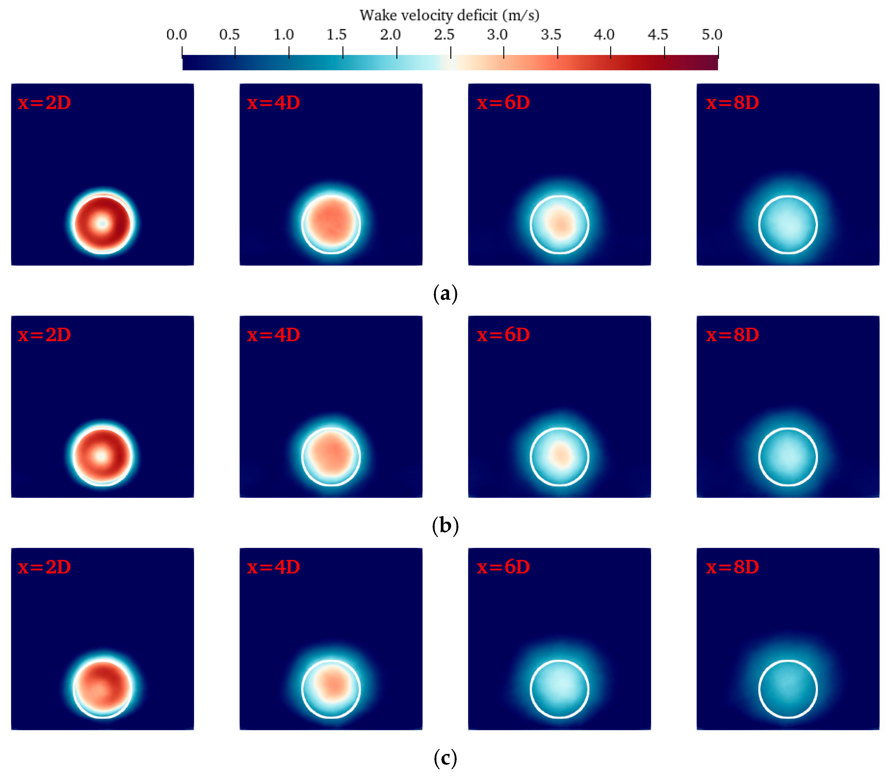
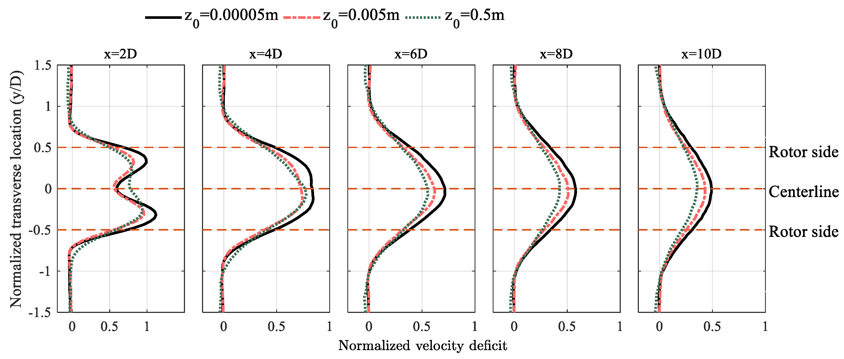
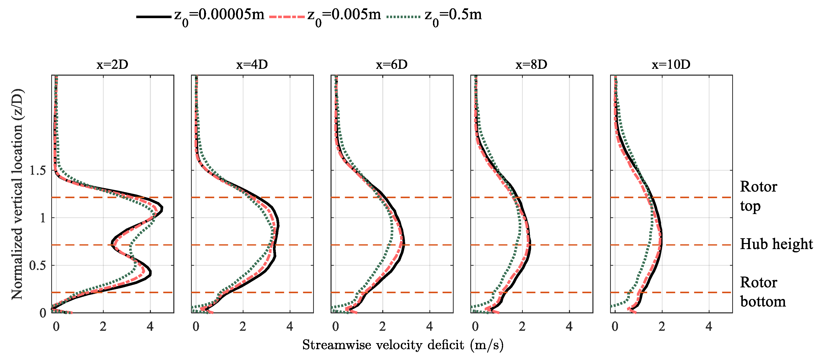
4.3. Mean Velocity Deficit

The wind rotor extracts energy from the incoming wind, causing a velocity reduction that decreases the power output of downstream turbines. Therefore, studying the wake velocity deficit is important for improving the wind farms layout, predicting power generation, and assessing the loads of turbines located in the wake region.

First, we discuss the mean statistics of the wake velocity. Figure 15 provides contours of the wake velocity deficit in vertical cross-sections under different roughness length conditions. The lateral direction is the y-axis with the range of −1.5D to 1.5D and the perpendicular direction is the z-axis. In this figure, the silver circle represents the swept circumference of wind rotor. Figure 15 illustrates that the velocity deficit is generally symmetrically distributed about y = 0 for all terrain conditions. Within the near-wake region, there is a ring-shaped contour of velocity deficit. Since the turbine blades have primarily circular cross-sections near their roots for structural rigidity, the velocity deficit is small near the wake center. Comparing the contours under different roughness length conditions, we find that as the roughness increases, the near wake merges more quickly and the far wake recovers faster. This is because an increase in roughness leads to an increase in turbulence of ABL wind, which accelerates the mixing process between the wake and the ambient atmosphere, thus resulting in a faster recovery of the wake.

Figure 16 gives the horizontal contours of the wake velocity deficit at hub height. From Figure 16, it becomes more evident that close to the wind turbine, the wake velocity deficit is concentrated on the two sides. As the wake develops, the velocity deficits on the sides gradually converge towards the centerline of the wake, and they meet around 3D to 4D downstream. This distance is not fixed and is mainly affected by the ambient atmospheric conditions and the thrust coefficient. As roughness length increases, the velocity deficits on the sides merge more quickly at the centerline of the wake. Moreover, from the velocity contours, we can observe that with increasing roughness length, the velocity deficit recovers faster, and the wake expands in width.

To quantitatively evaluate the velocity deficit under different roughness length, Figure 17 provides velocity deficit profiles at hub height for different downstream positions. From Figure 17, we can observe that at 2D downstream, the near-wake velocity deficit exhibits a bimodal distribution, which then converges towards the centerline as the wake progresses downstream. This convergence occurs around 3D to 4D downstream. When comparing different roughness conditions longitudinally, it is clear that higher roughness leads to a quicker transition from the near wake to the far wake. While the near wake ends, the bimodal distribution disappears, and the velocity deficit resembles a top-hat distribution. Further downstream, the wake has developed into the far-wake state, and the velocity deficit takes on a normal Gaussian-like distribution. Comparing the wake velocity deficit profiles for different roughness length conditions, it can be seen that very close to the turbine, the velocity deficit is similar for all roughness conditions. However, as the wake progresses downstream, the effect of atmospheric turbulence becomes apparent. Additionally, it is observed that beyond the 6D, the greater the roughness length, the smaller the velocity deficit. However, there is no noticeable difference in the numerical simulation results for time steps of 0.005 m and 0.00005 m. We think that the reason for this phenomenon is the difference in thrust coefficient between these two cases.

To address this issue, we adopt a dimensionless method to highlight the impact of roughness length. The non-dimensional form of the velocity deficit can be provided by the expression:

$$\tilde{U}={\displaystyle \frac{U_{\infty }-U_W}{U_D}}$$

(6)

where $U_D$ is the wind speed at the wind turbine location, $U_D=U_{\infty }\left(1-\sqrt{1-C_T}\right)$. Figure 18 provides the non-dimensional velocity deficit profiles. From the figure, it is evident that at far-wake positions, the influence of roughness length is quite pronounced, especially when comparing the cases of 0.00005 m and 0.005 m. These differences are more significant than those shown in the previous Figure 17.

Figure 19 provides vertical cross-sections of the velocity deficit at different downstream locations. Similarly to the results in the horizontal plane, as roughness length increases and incoming turbulence intensifies, the velocity deficit values become smaller. At the downstream position of 2D, we can observe that under lower roughness conditions, the two peaks in the velocity deficit profile are roughly of equal magnitude. However, under higher roughness conditions, the upper part of the wake has a larger velocity deficit than the lower part. This can be explained by the fact that, under higher roughness length, the turbulence near the terrain is greater, leading to a faster mixing rate between the lower part of the wake and the external environment compared to the upper part of the wake, which results in this phenomenon. In the far-wake region, the vertical cross-section of the velocity deficit is similar to that in the horizontal plane, i.e., the greater the roughness length, the smaller the velocity deficit values.

Figure 20 presents the vertical profiles of the velocity deficit at different downstream positions. At the position of 2D, we observe that under lower roughness conditions, the difference between the two peaks of the bimodal distribution is relatively small, with a difference of about 0.5 m/s. However, under higher roughness conditions, the velocity deficit in the upper half of the wake is significantly greater than in the lower half. This can be attributed to the increased turbulence near the terrain in higher roughness conditions, leading to a faster mixing rate of the lower part of the wake with the external environment compared to the upper part, thus causing this phenomenon. At the far-wake positions, the vertical profiles of the velocity deficit are similar to the horizontal cross-sections: the greater the roughness length, the smaller the velocity deficit values. However, we notice that for roughness values of 0.00005 m and 0.005 m, the maximum velocity deficit still occurs near the hub height. In contrast, for a roughness value of 0.5 m, the vertical position of the maximum velocity deficit has shifted from the hub height to the rotor-top height. Therefore, it can be concluded that as roughness length increases, the wake center will experience a vertical offset. Furthermore, above the hub height, the velocity deficit profile is similar to a Gaussian function; however, below the hub height, the Gaussian function may not accurately describe the distribution of the velocity deficit because the velocity deficit on the ground should be zero. This kind of error might be small in the near wake but becomes significant in the far wake. Both phenomena need to be taken into account in future analytical models.

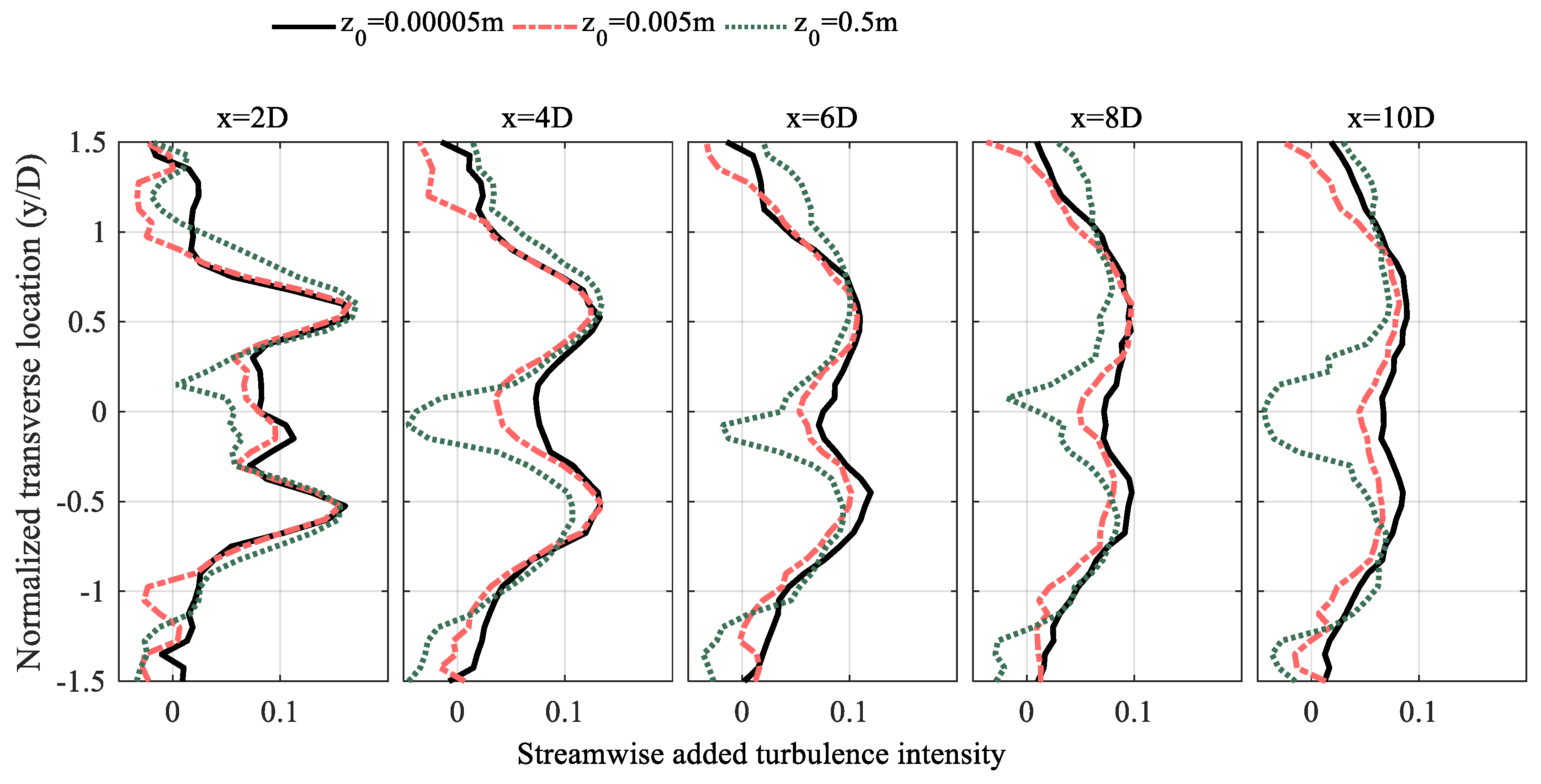
4.4. Turbulence Intensity

Since wind turbines extract kinetic energy from the wind, an added velocity gradient will be generated between the wake region and the ambient ABL wind, which increases the turbulence intensity. Generally, the portion of increased turbulence intensity is referred to as added turbulence intensity (ATI). The increase in turbulence intensity within the wake affects both the recovery rate of the wake and the fatigue loads on downstream wind turbines. This makes the study of turbulence intensity in the wake region particularly important.

Figure 21 shows the vertical cross-section diagrams of wake streamwise turbulence intensity under different roughness length conditions. From Figure 21, it can be observed that at x = 2D, turbulence is mainly distributed around the circumference of the blade’s swept area and at the circumference swept out from the blade root. At this time, the dominant increase in turbulence intensity is due to the breakup of the vortex systems. As the wake develops, the influence of the root vortex disappears, and the broken tip vortices gradually merge with the external environment. The influencing range of ATI begins to expand, extending not only toward the center of the wake but also outward the wake boundary. In the far wake region, the distribution of wake turbulence intensity exhibits a clear asymmetry concerning the hub height. In the middle to lower part of the far wake, a region of reduced turbulence intensity appears. The reason for this phenomenon is that within this range, the existence of wake velocity deficit results in suppressing the velocity shear with height, which decreases turbulence intensity. Comparing the turbulence intensity diagrams of the wake reveals that as roughness length increases, the turbulence intensity also increases, along with a larger affected area.

Figure 22 shows the horizontal contours of wake streamwise turbulence intensity at hub height under different surface roughness. From Figure 22, it can be observed that, like the velocity deficit, the turbulence intensity in the wake exhibits a symmetrical distribution about the centerline. In the near-wake region, the ATI is primarily concentrated at the lateral position where the blade tip is located. As the wake progresses downstream, the tip vortices begin to break up. Approximately between 2D and 4D, the turbulence intensity in the wake reaches its maximum value, which is consistent with the experimental finding from Ref. [59]. When within the far wake region, the turbulence intensity gradually starts to decrease as the wake recovers, although the affected range expands. At this point, the ATI is mainly caused by the extra wind speed shear resulting from the wake velocity deficit.

To better analyze the increased part, Figure 23 presents transverse profiles of ATI at hub height. From Figure 23, it can be observed that two significant peaks appear at the position of $y=\pm 0.5D$, caused by the shedding of tip vortices within the near wake. Additionally, a smaller peak is observed near the blade root, which may be produced by the breakup of root vortices. The profiles at 2D show that in the near-wake, the effect of roughness length on ATI is not significant. As the wake gradually develops downstream, the ATI resulted from the root vortices disappears, and the ATI near the blade tip gradually decreases and begins to merge toward the sides. When the wake reaches the far wake stage, all broken vortex structures merge with the environment. At this point, the ATI is primarily produced by the velocity shear of the wake, exhibiting a bimodal distribution. As the ATI evolves with the wake, the range of influence of wake turbulence intensity increases, but the maximum value gradually decreases. This is because the wake velocity deficit gradually diminishes, and the wake width also increases, leading to a gradual weakening of velocity shear, which in turn reduces the amplitude of ATI. Overall, the greater the environmental turbulence intensity, the smaller the ATI in the wake.

Figure 24 presents the vertical contours of turbulence intensity along the centerline under different roughness length conditions. From Figure 24, it can be seen that the turbulence intensity is asymmetric concerning hub height. The turbulence intensity above hub height is distinctively greater compared to that in the lower part of the wake. From these contours, it is evident that when the roughness length is 0.00005 m and 0.005 m, the turbulence intensity in the wake clearly increases. However, under the condition of 0.5 m roughness length, the turbulence intensity below hub height decreases compared to the inflow conditions.

To better quantitatively analyze the vertical distributions, Figure 25 presents the vertical profiles of ATI with height. It can be seen that the ATI exhibits a vertical distribution feature that first increases and then decreases with height. We can observe that below hub height, when ${\mathrm{z}}_0=0.5 \mathrm{m}$, there is a significant negative value of ATI. This phenomenon is due to the presence of the velocity deficit, which, compared to the external ABL, suppresses the wind speed shear with height. As the roughness decreases, when ${\mathrm{z}}_0=0.005 \mathrm{m}$, the wind shear in the external ABL becomes smaller compared to the 0.5 m condition, resulting in both the value and range of the negative ATI becoming smaller. Furthermore, compared to the results from Ref. [16], the present results give a more noticeable negative value for ATI at hub height when ${\mathrm{z}}_0=0.5 \mathrm{m}$. Perhaps these differences require further in-depth investigation in the future.

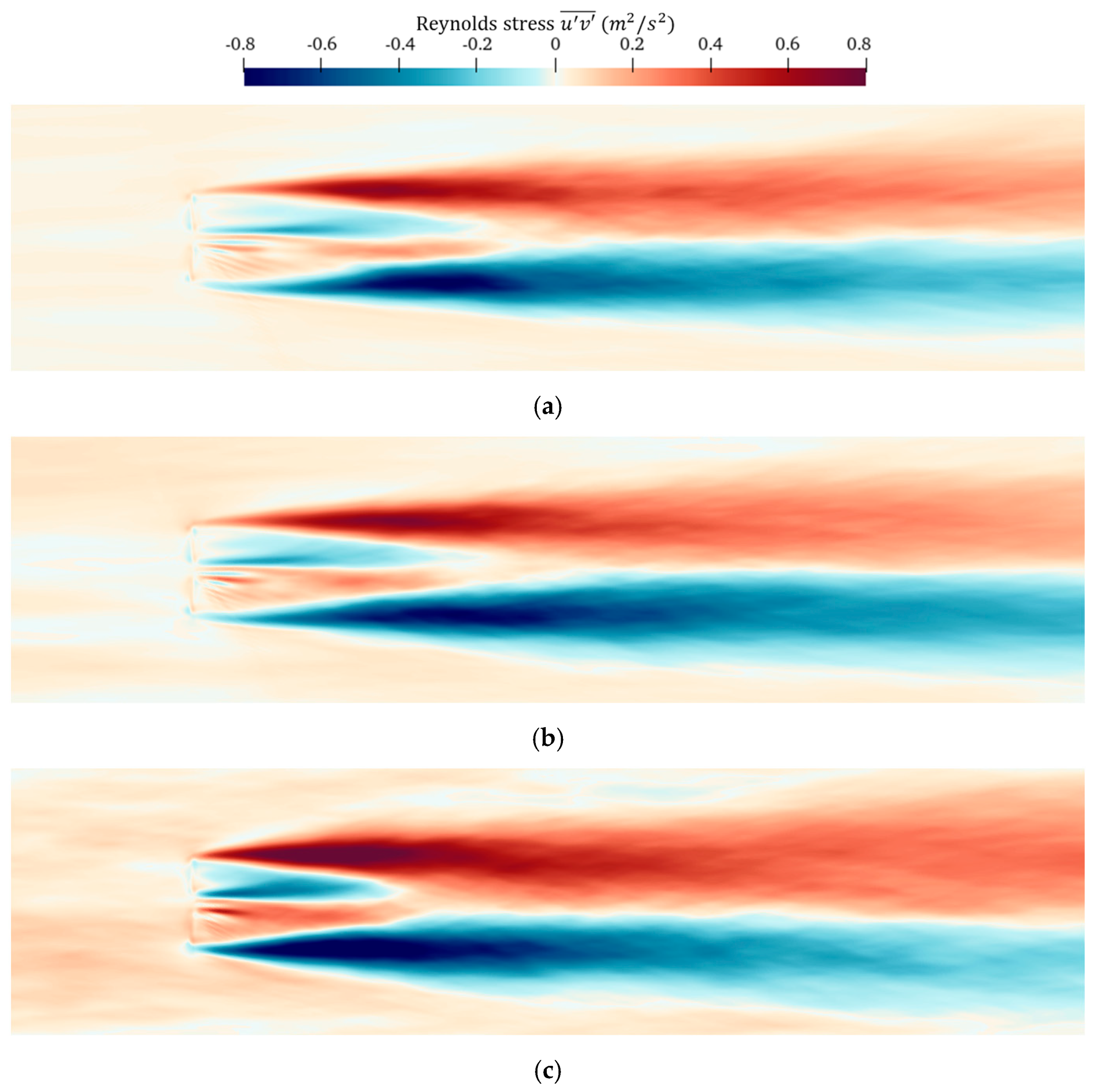
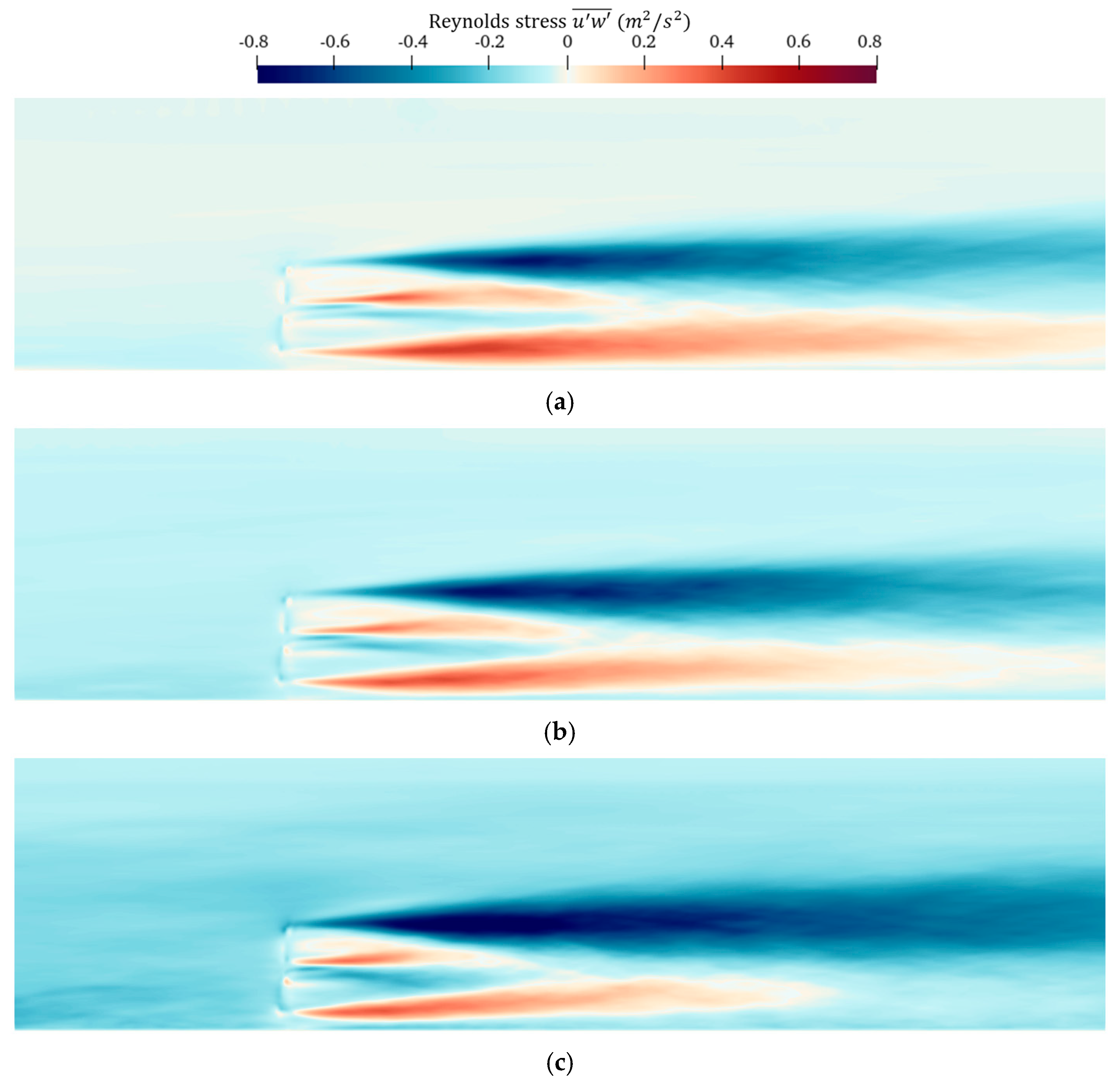
4.5. Reynolds Shear Stress

Next, we discuss the Reynolds shear stress within the wind turbine wake. The Reynolds shear stress influences the recovery of the wake velocity deficit. Figure 26 shows the horizontal distribution contours of Reynolds shear stress $\overline{u\prime v\prime }$ at the hub height. This component primarily dominates the mixing of the wake with the external environment in the horizontal direction. Figure 26 indicates that the Reynolds shear stress is basically symmetrically distributed about the wake centerline. Similarly to the turbulence intensity, the $\overline{u\prime v\prime }$ increases from the blade tips and roots, and as the wake develops downstream, its value first increases and then decreases, but the influencing area continues to expand. Furthermore, we can obtain that the magnitude of the Reynolds shear stress rises with greater roughness length. This suggests that under higher roughness length, the Reynolds shear stress is stronger, which accelerates the momentum mixing between the wake and the external ABL flow, thereby further speeding up the recovery of the wake.

To quantitatively compare the $\overline{u\prime v\prime }$ under different conditions, Figure 27 provides a comparison of the hub-height profiles for $\overline{u\prime v\prime }$ at different downstream positions. Under the three conditions, the wake is essentially antisymmetric about y = 0. The positive and negative values of the $\overline{u\prime v\prime }$ indicate the direction of mixing between the wake and the external environment, rather than the magnitude itself. From the figure, it can be observed that the Reynolds shear stress increases with increasing roughness length. At x = 2D, there are four extrema, which is due to the influence of the root vortices still being present; however, this influence disappears after 4D. In the range of x = 6D to 10D, the $\overline{u\prime v\prime }$ in the wake does not show significant differences. The author believes that this may be due to two overlapping reasons: (1) One reason is that when the roughness length is higher, the wake recovers more quickly, resulting in smaller velocity deficits compared to lower roughness conditions; (2) Another reason is that the background turbulent viscosity is higher under greater roughness conditions.

We then observe another component of the Reynolds shear stress, namely $\overline{u\prime w\prime }$. Figure 28 gives the vertical cross-section contours of $\overline{u\prime w\prime }$. This component primarily governs the mixing of the wake with the external environment in the vertical direction. From Figure 28, it can be observed that the $\overline{u\prime w\prime }$ above the hub height and below the hub height have opposite signs. This indicates that in the upper half of the wake, the direction of momentum exchange with the environment is from top to bottom, while in the lower half of the wake, the direction of momentum exchange is from bottom to top. Additionally, it can be seen that the $\overline{u\prime w\prime }$ above the hub height is greater than below the hub height, suggesting that the mixing in the upper half is more intense than in the lower half. Furthermore, as the roughness length increases, the mixing length in the lower half becomes shorter. This indicates that with increasing roughness length, the turbulent mixing near the ground occurs more rapidly, further enhancing the asymmetry of the wake.

Next, we quantitatively compare the added $\Delta \overline{u\prime w\prime }$ under different roughness conditions, which is calculated by $\Delta \overline{u\prime w\prime }=\overline{u\prime w\prime }-{\overline{u\prime w\prime }}_{\infty }(z)$. Figure 29 shows the profiles of $\Delta \overline{u\prime w\prime }$ varying with height. We can find that at x = 2D, the peak values of added Reynolds shear stress for three roughness conditions are quite close. The stress at the bottom of the rotor is approximately 0.5, while at the top of the rotor, it is around −0.6. As the wake progresses, it is evident that the region below the hub height recovers more quickly than the region above the hub height. However, overall, the differences in added Reynolds shear stress between different roughness conditions are not significant in the far wake. The reasons for this phenomenon are discussed in the above paragraph. For future work, it is necessary to systematically explore the effects of incoming flow conditions and thrust coefficient on the Reynolds shear stress of wind turbine wake. This will provide deeper insights into the turbulence mechanisms of wind turbine wake.

5. Conclusions

In this study, the LES-ALM is used to simulate the wake features of a single wind turbine within the ABL wind field under different roughness length conditions. The following conclusions can be drawn:

(1)

Larger time step can be used for the numerical simulation of LES-ALM. As the time step increases, the thrust and power slightly decrease. However, the effects on the turbulent characteristics of the wake are not significant.

(2)

As roughness length increases, the fluctuations in thrust and power become more intense. Under the same hub-height wind speed, the turbine has the highest thrust coefficient of 0.82 when the roughness length is 0.005 m which is notably higher than the other two cases. Therefore, when analyzing the impacts of roughness length on the wake, the effects on the thrust coefficient should be considered.

(3)

The greater the roughness length, the more intense the environmental turbulence, leading to the faster recovery of velocity deficit and ATI within the wake. For the velocity deficit, a single Gaussian function is not able to describe its vertical distribution. Additionally, numerical simulation results reveal that when the roughness length is 0.5 m, the height of the wake center is significantly higher than the hub height. Thus, in future analytical models, the variation in the wake center with height should be considered to ensure the accuracy of model predictions.

(4)

Numerical simulations show that as roughness length increases, the Reynolds shear stress in the wake also increases, but the differences are not significant. Due to wind shear effects, the recovery of the added Reynolds shear stress component $\Delta \overline{u\prime w\prime }$ below the hub height is faster than above the hub height.

References

- GWEC. Global Wind Report 2023|GWEC; GWEC: Brussels, Belgium, 2023. [Google Scholar]
- Tian, W.; Wei, F.; Zhao, Y.; Wan, J.; Zhao, X.; Liu, L.; Zhang, L. A Numerical Investigation of the Influence of the Wake for Mixed Layout Wind Turbines in Wind Farms Using FLORIS. J. Mar. Sci. Eng. 2024, 12, 1714. [Google Scholar] [CrossRef]
- Cui, J.; Wu, X.; Lyu, P.; Zhao, T.; Li, Q.; Ma, R.; Liu, Y. Research on the Power Output of Different Floating Wind Farms Considering the Wake Effect. J. Mar. Sci. Eng. 2024, 12, 1475. [Google Scholar] [CrossRef]
- Chowdhury, S.; Zhang, J.; Messac, A.; Castillo, L. Optimizing the Arrangement and the Selection of Turbines for Wind Farms Subject to Varying Wind Conditions. Renew. Energy 2013, 52, 273–282. [Google Scholar] [CrossRef]
- Gupta, N. A Review on the Inclusion of Wind Generation in Power System Studies. Renew. Sustain. Energy Rev. 2016, 59, 530–543. [Google Scholar] [CrossRef]
- Porté-Agel, F.; Bastankhah, M.; Shamsoddin, S. Wind-Turbine and Wind-Farm Flows: A Review. Bound.-Layer Meteorol. 2020, 174, 1–59. [Google Scholar] [CrossRef]
- Barthelmie, R.J.; Hansen, K.; Frandsen, S.T.; Rathmann, O.; Schepers, J.G.; Schlez, W.; Phillips, J.; Rados, K.; Zervos, A.; Politis, E.S.; et al. Modelling and Measuring Flow and Wind Turbine Wakes in Large Wind Farms Offshore. Wind Energy 2009, 12, 431–444. [Google Scholar] [CrossRef]
- Barthelmie, R.J.; Pryor, S.C.; Frandsen, S.T.; Hansen, K.S.; Schepers, J.G.; Rados, K.; Schlez, W.; Neubert, A.; Jensen, L.E.; Neckelmann, S. Quantifying the Impact of Wind Turbine Wakes on Power Output at Offshore Wind Farms. J. Atmos. Ocean. Technol. 2010, 27, 1302–1317. [Google Scholar] [CrossRef]
- Barthelmie, R.J.; Folkerts, L.; Larsen, G.C.; Rados, K.; Pryor, S.C.; Frandsen, S.T.; Lange, B.; Schepers, G. Comparison of Wake Model Simulations with Offshore Wind Turbine Wake Profiles Measured by Sodar. J. Atmos. Ocean. Technol. 2006, 23, 888–901. [Google Scholar] [CrossRef]
- Thomsen, K.; Sørensen, P. Fatigue Loads for Wind Turbines Operating in Wakes. J. Wind Eng. Ind. Aerodyn. 1999, 80, 121–136. [Google Scholar] [CrossRef]
- Li, L.; Huang, Z.; Ge, M.; Zhang, Q. A Novel Three-Dimensional Analytical Model of the Added Streamwise Turbulence Intensity for Wind-Turbine Wakes. Energy 2022, 238, 121806. [Google Scholar] [CrossRef]
- Göçmen, T.; Van Der Laan, P.; Réthoré, P.E.; Diaz, A.P.; Larsen, G.C.; Ott, S. Wind Turbine Wake Models Developed at the Technical University of Denmark: A Review. Renew. Sustain. Energy Rev. 2016, 60, 752–769. [Google Scholar] [CrossRef]
- Ghafoorian, F.; Mirmotahari, S.R.; Bakhtiari, F.; Mehrpooya, M. Exploring Optimal Configurations for a Wind Farm with Clusters of Darrieus VAWT, Using CFD Methodology. J. Comput. Appl. Mech. 2023, 54, 533–551. [Google Scholar] [CrossRef]
- Chegini, S.; Ghafoorian, F.; Moghimi, M.; Mehrpooya, M. Optimized Arrangement of Clustered Savonius VAWTs, Techno-Economic Evaluation, and Feasibility of Installation. Iran. J. Chem. Chem. Eng. 2024, 43, 875–894. [Google Scholar] [CrossRef]
- Churchfield, M.J.; Lee, S.; Michalakes, J.; Moriarty, P.J. A Numerical Study of the Effects of Atmospheric and Wake Turbulence on Wind Turbine Dynamics. J. Turbul. 2012, 13, N14. [Google Scholar] [CrossRef]
- Wu, Y.-T.; Porté-Agel, F. Atmospheric Turbulence Effects on Wind-Turbine Wakes: An LES Study. Energies 2012, 5, 5340–5362. [Google Scholar] [CrossRef]
- Stein, V.P.; Kaltenbach, H.J. Influence of Ground Roughness on the Wake of a Yawed Wind Turbine—A Comparison of Wind-Tunnel Measurements and Model Predictions. Proc. J. Phys. Conf. Ser. 2018, 1037, 072005. [Google Scholar] [CrossRef]
- Stein, V.P.; Kaltenbach, H.J. Validation of a Large-Eddy Simulation Approach for Prediction of the Ground Roughness Influence on Wind Turbine Wakes. Energies 2022, 15, 2579. [Google Scholar] [CrossRef]
- Rotich, I.K.; Chepkirui, H. Study on Influence of Turbulence Intensity on Blade Airfoil Icing Mass & Aerodynamic Performance. Heliyon 2024, 10, e31859. [Google Scholar] [CrossRef]
- Ismaiel, A. Rotor Dynamics of AWT-27 Two-Bladed Wind Turbine Under Turbulence Effect. Int. Rev. Mech. Eng. 2022, 16, 373. [Google Scholar] [CrossRef]
- Manwell, J.F.; McGowan, J.G.; Rogers, A.L. Wind Energy Explained: Theory, Design and Application; John Wiley & Sons: Hoboken, NJ, USA, 2010. ISBN 978047001 5001.
- Stevens, R.J.A.M.; Martínez-Tossas, L.A.; Meneveau, C. Comparison of Wind Farm Large Eddy Simulations Using Actuator Disk and Actuator Line Models with Wind Tunnel Experiments. Renew. Energy 2018, 116, 470–478. [Google Scholar] [CrossRef]
- Fu, C.; Zhang, Z.; Yu, M.; Zhou, D.; Zhu, H.; Duan, L.; Tu, J.; Han, Z. Research on Aerodynamic Characteristics of Three Offshore Wind Turbines Based on Large Eddy Simulation and Actuator Line Model. J. Mar. Sci. Eng. 2024, 12, 1341. [Google Scholar] [CrossRef]
- Tu, Y.; Zhang, K.; Han, Z.; Zhou, D.; Bilgen, O. Aerodynamic Characterization of Two Tandem Wind Turbines under Yaw Misalignment Control Using Actuator Line Model. Ocean Eng. 2023, 281, 114992. [Google Scholar] [CrossRef]
- Martínez-Tossas, L.A.; Churchfield, M.J.; Meneveau, C. Large Eddy Simulation of Wind Turbine Wakes: Detailed Comparisons of Two Codes Focusing on Effects of Numerics and Subgrid Modeling. Proc. J. Phys. Conf. Ser. 2015, 625, 012024. [Google Scholar] [CrossRef]
- Wu, Y.-T.; Porté-Agel, F. Large-Eddy Simulation of Wind-Turbine Wakes: Evaluation of Turbine Parametrisations. Boundary-Layer Meteorol. 2011, 138, 345–366. [Google Scholar] [CrossRef]
- Troldborg, N.; Sorensen, J.N.; Mikkelsen, R. Numerical Simulations of Wake Characteristics of a Wind Turbine in Uniform Inflow. Wind Energy 2010, 13, 86–99. [Google Scholar] [CrossRef]
- Troldborg, N. Actuator Line Modeling of Wind Turbine Wakes. Ph.D. Thesis, Technical University of Denmark, Lyngby, Denmark, 2008. [Google Scholar]
- Martínez, L.A.; Leonardi, S.; Churchfield, M.J.; Moriarty, P.J. A Comparison of Actuator Disk and Actuator Line Wind Turbine Models and Best Practices for Their Use. In Proceedings of the 50th AIAA Aerospace Sciences Meeting Including the New Horizons Forum and Aerospace Exposition, Nashville, TN, USA, 9–12 January 2012. [Google Scholar]
- Bastankhah, M.; Porté-Agel, F. Experimental and Theoretical Study of Wind Turbine Wakes in Yawed Conditions. J. Fluid Mech. 2016, 806, 506–541. [Google Scholar] [CrossRef]
- Bastankhah, M.; Porté-Agel, F. A New Miniaturewind Turbine for Wind Tunnel Experiments. Part II: Wake Structure and Flow Dynamics. Energies 2017, 10, 923. [Google Scholar] [CrossRef]
- Jensen, N.O. A Note on Wind Generator Interaction. In Risø-M-2411 Risø National Laboratory. Risø-M; DTU: Roskilde, Denmark, 1983. [Google Scholar]
- Bastankhah, M.; Porté-Agel, F. A New Analytical Model for Wind-Turbine Wakes. Renew. Energy 2014, 70, 116–123. [Google Scholar] [CrossRef]
- Ishihara, T.; Qian, G.W. A New Gaussian-Based Analytical Wake Model for Wind Turbines Considering Ambient Turbulence Intensities and Thrust Coefficient Effects. J. Wind Eng. Ind. Aerodyn. 2018, 177, 275–292. [Google Scholar] [CrossRef]
- Sun, H.; Yang, H. Study on an Innovative Three-Dimensional Wind Turbine Wake Model. Appl. Energy 2018, 226, 483–493. [Google Scholar] [CrossRef]
- Zhang, S.; Gao, X.; Ma, W.; Lu, H.; Lv, T.; Xu, S.; Zhu, X.; Sun, H.; Wang, Y. Derivation and Verification of Three-Dimensional Wake Model of Multiple Wind Turbines Based on Super-Gaussian Function. Renew. Energy 2023, 215, 118968. [Google Scholar] [CrossRef]
- Tian, L.; Xiao, P.; Song, Y.; Zhao, N.; Zhu, C.; Lu, X. An Advanced Three-Dimensional Analytical Model for Wind Turbine near and Far Wake Predictions. Renew. Energy 2024, 223, 120035. [Google Scholar] [CrossRef]
- Ge, M.; Wu, Y.; Liu, Y.; Li, Q. A Two-Dimensional Model Based on the Expansion of Physical Wake Boundary for Wind-Turbine Wakes. Appl. Energy 2019, 233–234, 975–984. [Google Scholar] [CrossRef]
- Yang, Q.; Liu, G.; Qian, Y. A Yawed Wake Model to Predict the Velocity Distribution of Curled Wake Cross-Section for Wind Turbines. Ocean Eng. 2024, 295, 116911. [Google Scholar] [CrossRef]
- Cheng, Y.; Zhang, M.; Zhang, Z.; Xu, J. A New Analytical Model for Wind Turbine Wakes Based on Monin-Obukhov Similarity Theory. Appl. Energy 2019, 239, 96–106. [Google Scholar] [CrossRef]
- Abdelsalam, A.M.; Boopathi, K.; Gomathinayagam, S.; Hari Krishnan Kumar, S.S.; Ramalingam, V. Experimental and Numerical Studies on the Wake Behavior of a Horizontal Axis Wind Turbine. J. Wind Eng. Ind. Aerodyn. 2014, 128, 54–65. [Google Scholar] [CrossRef]
- Chamorro, L.P.; Porté-Agel, F. A Wind-Tunnel Investigation of Wind-Turbine Wakes: Boundary-Layer Turbulence Effects. Bound.-Layer Meteorol. 2009, 132, 129–149. [Google Scholar] [CrossRef]
- Zhang, L.; Feng, Z.; Zhao, Y.; Xu, X.; Feng, J.; Ren, H.; Zhang, B.; Tian, W. Experimental Study of Wake Evolution under Vertical Staggered Arrangement of Wind Turbines of Different Sizes. J. Mar. Sci. Eng. 2024, 12, 434. [Google Scholar] [CrossRef]
- Cleijne, J.W. Results of Sexbierum Wind Farm; Single Wake Measurements; TNO: Delft, The Netherlands, 1993. [Google Scholar]
- Li, Z.; Pu, O.; Pan, Y.; Huang, B.; Zhao, Z.; Wu, H. A Study on Measuring Wind Turbine Wake Based on UAV Anemometry System. Sustain. Energy Technol. Assess. 2022, 53, 102537. [Google Scholar] [CrossRef]
- Xie, S.; Archer, C. Self-Similarity and Turbulence Characteristics of Wind Turbine Wakes via Large-Eddy Simulation. Wind Energy 2015, 18, 1815–1838. [Google Scholar] [CrossRef]
- Li, L.; Wang, B.; Ge, M.; Huang, Z.; Li, X.; Liu, Y. A Novel Superposition Method for Streamwise Turbulence Intensity of Wind-Turbine Wakes. Energy 2023, 276, 127491. [Google Scholar] [CrossRef]
- Tian, L.; Song, Y.; Xiao, P.; Zhao, N.; Shen, W.; Zhu, C. A New Three-Dimensional Analytical Model for Wind Turbine Wake Turbulence Intensity Predictions. Renew. Energy 2022, 189, 762–776. [Google Scholar] [CrossRef]
- Huang, L.; Tang, H.; Zhang, K.; Fu, Y.; Liu, Y. 3-D Layout Optimization of Wind Turbines Considering Fatigue Distribution. IEEE Trans. Sustain. Energy 2020, 11, 126–135. [Google Scholar] [CrossRef]
- Zhao, R.; Shen, W.; Knudsen, T.; Bak, T. Fatigue Distribution Optimization for Offshore Wind Farms Using Intelligent Agent Control. Wind Energy 2012, 15, 927–944. [Google Scholar] [CrossRef]
- Fleming, P.A.; Gebraad, P.M.O.; Lee, S.; van Wingerden, J.W.; Johnson, K.; Churchfield, M.; Michalakes, J.; Spalart, P.; Moriarty, P. Evaluating Techniques for Redirecting Turbine Wakes Using SOWFA. Renew. Energy 2014, 70, 211–218. [Google Scholar] [CrossRef]
- Burton, T.; Jenkins, N.; Sharpe, D.; Bossanyi, E. Wind Energy Handbook, 2nd ed.; John Wiley & Sons: Hoboken, NJ, USA, 2011; ISBN 9780470699751. [Google Scholar]
- Ghafoorian, F.; Enayati, E.; Mirmotahari, S.R.; Wan, H. Self-Starting Improvement and Performance Enhancement in Darrieus VAWTs Using Auxiliary Blades and Deflectors. Machines 2024, 12, 806. [Google Scholar] [CrossRef]
- Munters, W.; Meneveau, C.; Meyers, J. Shifted Periodic Boundary Conditions for Simulations of Wall-Bounded Turbulent Flows. Phys. Fluids 2016, 28, 025112. [Google Scholar] [CrossRef]
- Schumann, U. Subgrid Scale Model for Finite Difference Simulations of Turbulent Flows in Plane Channels and Annuli. J. Comput. Phys. 1975, 18, 376–404. [Google Scholar] [CrossRef]
- Chamorro, L.P.; Porté-Agel, F. Effects of Thermal Stability and Incoming Boundary-Layer Flow Characteristics on Wind-Turbine Wakes: A Wind-Tunnel Study. Bound.-Layer Meteorol. 2010, 136, 515–533. [Google Scholar] [CrossRef]
- Deskos, G.; Laizet, S.; Piggott, M.D. Turbulence-Resolving Simulations of Wind Turbine Wakes. Renew. Energy 2019, 134, 989–1002. [Google Scholar] [CrossRef]
- Troldborg, N.; Sørensen, J.N.; Mikkelsen, R.; Sørensen, N.N. A Simple Atmospheric Boundary Layer Model Applied to Large Eddy Simulations of Wind Turbine Wakes. Wind Energy 2014, 17, 657–669. [Google Scholar] [CrossRef]
- Zhang, W.; Markfort, C.D.; Porté-Agel, F. Wind-Turbine Wakes in a Convective Boundary Layer: A Wind-Tunnel Study. Bound.-Layer Meteorol. 2013, 146, 161–179. [Google Scholar] [CrossRef]