Estimation and Characteristics of Low-Frequency Ambient Sea Noise from Far-Field Ships

Abstract

To study the rapid estimation method and characteristics of low-frequency ambient sea noise generated by far-field ships, firstly, based on the reciprocity principle of sound fields and the fact that the number of noise sources significantly exceeds the number of receiving array elements, the positions of noise sources and receiving array elements were swapped to effectively reduce the sound field estimates and the running time. Secondly, a vertical directionality analysis method for ambient noise generated by ship noise was derived. And lastly, the ambient sea noise generated by ship noise in the Philippine Sea was estimated and analyzed, and the validity of the estimation method was verified based on measured data in the region. The estimation method presented in this paper can be used to predict the level and directionality of ambient noise generated by ship noise in a large area of sea, and acts as technical support for the meaningful use of sonar arrays in the actual marine environment.

1. Introduction

Ship noise is a source of ambient noise interfering with underwater sonar arrays. With its acting range calculated by the sonar equation, the ambient noise at sonar arrays needs to be estimated and analyzed. In addition, where the sonar signal processing method is adopted, the spatiotemporal statistical properties of ambient noise at sonar arrays should be fully explored, and the difference in the spatiotemporal statistical properties between signals and ambient noise should be utilized to achieve a higher signal-to-noise ratio of sonar and thus enhance the detectivity of sonar arrays, for the purpose of anti-interference. For example, non-directional ambient noise at sonar arrays can be suppressed by designing a narrow beam, while directional ambient noise can be suppressed by setting a beam groove scan or zero constraint. Therefore, studies on ambient noise at sonar arrays are crucial to improve the detection performance of sonar.

Mathematical models of ambient sea noise predict such noise, taking the noise level and directionality as a function of parameters such as frequency, depth, time, terrain, and seabed medium. Two statistical models for ambient noise and beam noise are available to forecast hydrophone-sensed average noise levels and low-frequency shipping noise characteristics of large-aperture, narrow-beam passive sonar systems, respectively. Cron et al. [1] first proposed a C/S model of sea noise fields based on the assumptions that noise sources are uniformly distributed across an infinite sea surface, and that seawater and the seabed are together a semi-infinite uniform space. Chapman [2] deduced the vertical correlation function of sea noise fields by considering the impact of seabed reflections on a C/S model basis. Buckingham [3] used a normal wave model to calculate the vertical correlation function and array gain of an ambient noise field in shallow sea with a uniform sound velocity profile and low-loss seabed. Kuperman et al. [4] proposed a layered sea wave model (K/I model) that utilized the full-wave theory to block noise transmission and took into account the contributions of far-field discrete and near-field continuous noise spectra. Carey et al. [5] coupled the parabolic equation model for propagation with sea surface noise sources to outline the distance-related vertical distribution of ambient sea noise fields. The Institute of Acoustics, Chinese Academy of Sciences, applied the approximation to the generalized term integral of normal wave eigenfunction to the propagation calculation of ambient noise fields [6,7].

Over the past 20 years, several numerical prediction models for ambient noise based on theoretical models have emerged [8]. In the US, there has been RANDI (Research Ambient Noise Directionality Mode), used to estimate the vertical and horizontal directionality of low-frequency ambient sea noise and explain the special mechanism of shallow sea ambient noise; DUNES (Directional Underwater Noise Estimates), used to estimate the directionality of ambient noise; and ANDES (Ambient Noise Directional Estimation System), mainly used for ambient noise modeling in shallow sea, including shipping density and sound velocity data, and estimating the changes in noise directionality with wind velocity and motion of discrete sound sources in a sound field. In the UK, there has been CANARY (Coherence and Ambient Noise for Arrays), which is a ray-theory-based model for ambient noise–noise coherence used for assessing sonar performance in range- and phase-dependent environments that treats noise sources as a plane rather than points. In recent years, based on the above models, ambient sea noise has been extensively studied [9,10,11,12] in terms of its variations with environmental factors such as depth, frequency, terrain, and ship density, as well as the vertical and horizontal directionality of noise.

This paper presents a fast estimation method for ambient noise at sonar arrays generated by ship noise according to the reciprocity principle of sound fields, through which the estimation efficiency was improved significantly upon the position swap of sound sources and receiving points, since the number of sound sources was much larger than that of the receiving points in the noise field modeling. Lastly, combined with the actual ambient sea conditions, the ambient sea noise generated by ship noise in the Philippine Sea was modeled, estimated and analyzed, and the validity of the estimation method presented in this paper was verified.

2. Ship Noise Estimation Method

The estimation of ship noise requires the analysis of a large area of sea, and far-field ships—hundreds to thousands of kilometers away from hydrophones or even further—are the main noise sources, which conforms to the far-field hypothesis of sound field propagation. Noise at any point in the sea is a superposition of uncorrelated sound waves traveling from all directions to that point. The far-field hypothesis determines that ship noise is stationary in both time and space.

The inclusion rules for the range of ship noise sources [12] are as follows: The circular area with a sonar array site $o$ as the center and $r_0-r_J$ as the radius is defined as the range of ship noise sources that contributes to ambient noise at the sonar array. 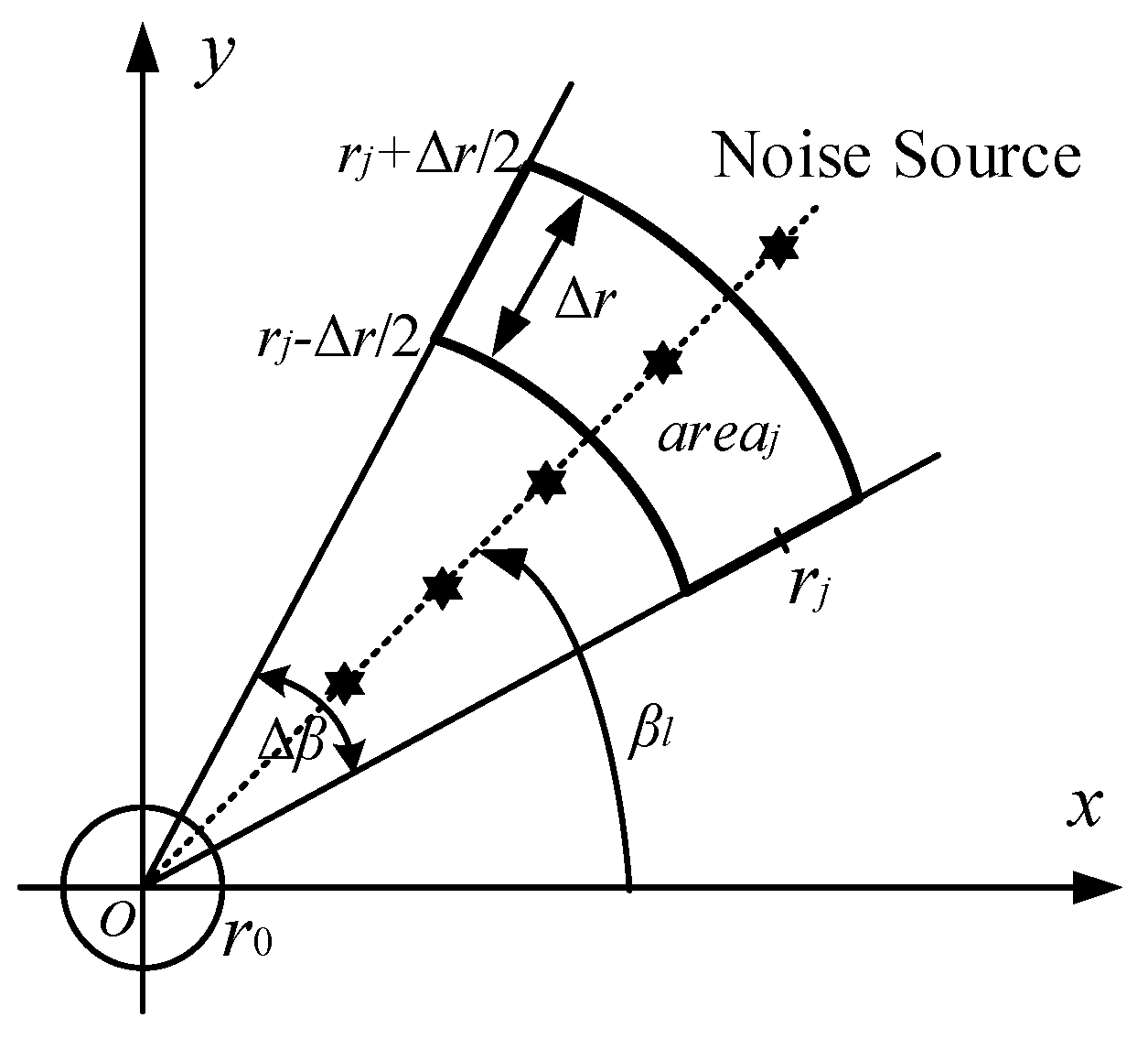The near-field ship noise within the sonar array $r_0$ should be analyzed separately as a discrete interference source, while the contribution of ship noise outside $r_J$ to ambient noise at the sonar array—subject to substantial attenuation of sound propagation over long distances—is negligible. As shown in Figure 1, the dark ringed area is the range of ship noise sources. Firstly, the ringed area is divided into L sectors with an equal angle and a radian of Δβ = 2π/L. Secondly, each sector is equally divided into J loops with a width of Δr, each of which is deemed as a ship noise surface source, totaling L × J. Lastly, the ambient noise at the sonar array can be estimated by superimposing the sound pressure generated by these sources at the sonar array.

Figure 2 is a diagram of the ambient noise estimation at the sonar array generated by the noise sources per unit intensity in the loops. With the receiving point of the sonar array, $\overline{x}=(x,y,z)$, located at the origin of coordinates, $o$, the complex sound pressure generated by a ship noise source with a depth of $z_s$, a distance of $r_j=r_0+j\cdot \Delta r$ (j = 1, 2, …, J), and an azimuth of ${\beta }_l=l\cdot \Delta \beta$ (l = 1, 2, …, L) at point $\overline{x}$ can be expressed as shown in Equation (1):

$$P_{j,l}(\overline{x})=n{s}_{jl}^2\cdot \sqrt{are{a}_j}\cdot u(f,\overline{x},r_j,z_s,{\beta }_l)$$

(1)

where $n{s}_{jl}^2={10}^{NS{L}_{jl}/10}$ is the noise intensity per unit area; $NS{L}_{\mathrm{jl}}$ is the sound intensity level at 1 m of the ship noise source, with 1 μPa²/Hz/m² as the reference value; $are{a}_j=\Delta \beta \cdot \Delta r\cdot r_j$ is the area of the $j$th loop; and $u(f,\overline{x},r_j,z_s,{\beta }_l)$ is the complex sound pressure generated by a unit-intensity sound source with a frequency of $f$, a depth of $z_s$, an azimuth of ${\beta }_l$, and a distance of $r_j$ at the receiving point $\overline{x}$ of the sonar array, which is estimated using sound field simulation software.

In real sea waveguides, the sea depth, sound velocity profile, and seabed parameters vary with distance, and, notably, sea depth varies more significantly. The parabolic equation model is quite effective for solving acoustic problems in waveguides that vary with distance. Figure 3 illustrates the direct estimation method for the sound field of a single sector in any waveguide that varies with distance, where H₁ is the sea depth at the sonar array and H₂ is the sea depth at a longer distance. For a vertical linear array with N_p array elements, only the normalized sound pressure of a single sound source on N_p receiving elements can be obtained for each estimation of the sound field. As terrain and noise intensity vary in different directions and locations, the sound field must be estimated separately for each noise source to obtain the overall sound pressure level of each array element; therefore, the direct method requires a total of M_D = J × L sound field estimations.

The principle of reciprocity is widely used in ambient noise numerical modelling [12,13]. According to the reciprocity of sound fields, the positions of the sound source and the receiving point are reversed, as shown in Figure 4. Upon each estimation of the sound field, the normalized sound pressure of a single sound source on J receiving array elements can be obtained. To obtain the overall sound pressure level of each array element, the sound field should be estimated M_R = Np × L times when using the reciprocity method.

If the estimated distance is expressed as R, the step length in distance as Δr, the sea depth at the sonar array as H₁, and the array element spacing as Δd, the ratio of the sound field estimates using the direct method to that using the reciprocal method is shown as Equation (2):

$${\displaystyle \frac{M_D}{M_R}}={\displaystyle \frac{R/\Delta r}{H_1/\Delta d}}\cdot {\displaystyle \frac{L}{L}}={\displaystyle \frac{R\cdot \Delta d}{H_1\cdot \Delta r}}$$

(2)

Because the estimated distance of ship noise is up to thousands of kilometers, and the number of receiving array elements is generally only dozens, the number of sound sources in a certain direction is far greater than the number of receiving array elements, resulting in a sharp drop in the sound field estimates. For example, the conditions of R = 3000 km (estimated distance), Δr = 1000 m, H₁ = 5 km (sea depth at the sonar array), and Δd = 200 m yield M_D/M_R = 120. To sum up, in sea waveguides varying with distance, the reciprocity method for estimating ship noise can greatly reduce the sound field estimates.

The noise sources in the ringed area in Figure 1 are added with random phase and superimposed according to the grid partitions of surface sources to obtain the complex sound pressure at the receiving point $\overline{x}$, as shown in Equation (3):

$$P(\overline{x})={\displaystyle \sum _{l=1}^L\exp (i{\psi }_l){\displaystyle \sum _{j=1}^J\exp (i{\psi }_j)n{s}_{j,l}}\sqrt{are{a}_j}P(\omega ,\overline{x},r_j,z_s,{\beta }_l)}$$

(3)

where ψ_l is the random phase in different directions and ψ_j is the random phase at different distances; both are uniformly distributed within [0, 2π].

3. Vertical Directionality of Ship Noise

The vertical structure and spatial directionality of ship noise not only reflect the spatial distribution of noise fields, but also act as a guide for the placement and mode of sonar arrays, which contributes to effectively weakening the impact of noise fields on the performance of sonar arrays. According to [13], for an arbitrarily shaped sonar array composed of N isotropic sensors, the positions of each array element are ${\mathit{p}}_n$ = (xn, yn, zn), (n = 1,2,…N). As shown in Figure 5, when the azimuth of the incident signal in a 3D rectangular coordinate system is $(\varphi ,\theta )$, the unit vector in this direction is shown in Equation (4):

$$\mathit{u}=\left[\begin{array}{c}\cos \varphi \cos \theta \\ \cos \varphi \sin \theta \\ \sin \varphi \end{array}\right]$$

(4)

and the response vector of signals in this direction is shown in Equation (5):

$$\mathit{v}(\varphi ,\theta )=\left[\begin{array}{c}\exp (-j\omega {\tau }_1(\varphi ,\theta ))\\ \exp (-j\omega {\tau }_2(\varphi ,\theta ))\\ ⋮\\ \exp (-j\omega {\tau }_N(\varphi ,\theta ))\end{array}\right]$$

(5)

where ${\tau }_n(\varphi ,\theta )$ is the time delay of the nth array element relative to the reference point of signals in the $(\varphi ,\theta )$ direction.

The wavenumber k is defined as shown in Equation (6).

$$\mathit{k}=-{\displaystyle \frac{\omega }{c}}\mathit{u}$$

(6)

and accordingly, the relative time delay on each array element can be expressed in Equation (7):

$${\tau }_{\mathrm{n}}={\mathit{k}}^T{\mathit{p}}_n/\omega$$

(7)

where ^(*)T stands for the presence of a transpose and ω is the angular frequency, i.e., ω = 2πf, in which f is the narrowband signal center frequency.

The manifold vector of the sonar array in this direction can be expressed as shown in Equation (8):

$$\mathit{v}(\mathit{k})=\left[\begin{array}{c}\exp (-j{\mathit{k}}^T{\mathit{p}}_1)\\ \exp (-j{\mathit{k}}^T{\mathit{p}}_2)\\ ⋮\\ \exp (-j{\mathit{k}}^T{\mathit{p}}_N)\end{array}\right]$$

(8)

Assuming that the complex sound pressure of N elements of the sonar array calculated using Equation (3) is ${\mathit{P}}_N=[P({\overline{x}}_1),P({\overline{x}}_2),\cdots ,P({\overline{x}}_N)]$, the covariance matrix of ship noise received by the sonar array can be expressed in Equation (9):

$${\mathit{R}}_N={\mathit{P}}_N^H\cdot {\mathit{P}}_N$$

(9)

As a result, the beam scanning azimuth spectrum, i.e., the function of beam output power relative to the azimuth obtained by scanning the beam observation direction, can be defined in Equation (10):

$$P(\varphi ,\theta )={\mathit{v}}^H(\mathit{k})\cdot {\mathit{R}}_N\cdot \mathit{v}(\mathit{k})$$

(10)

where ^(*)H stands for the presence of a conjugate transpose, and it generally takes the logarithm, i.e., $10\log P(\varphi ,\theta )$, when the azimuth spectrum is displayed.

4. Estimation and Validation of Ship Noise in the Philippine Sea

The Applied Physics Laboratory (APL), University of Washington, was sponsored by the Office of Naval Research to measure and study the seabed sediments, hydrological conditions, acoustic propagation properties, and ambient sea noise in the Philippine Sea [14]. Figure 6 shows a schematic of station selection during the experiment, in which stations T1, T2, T3, T4, and T5 were located at the five vertices of the regular pentagram, T6 was located at the center of the pentagram, and the Distributed Vertical Line Array (DVLA) (triangular position) was located in the northwest of T6.

From May 2010 to March 2011, APL estimated the ambient noise at station DVLA in an experiment [15] called “PhilSea10”. The vertical linear array used in this experiment is composed of 152 array elements and distributed throughout the sea depth. The vertical array consists of five 1000-m-long subarrays at a spacing of 20 m near the soundtrack axis or 40 m near the critical depth. The GPS coordinates of the seven stations in Figure 6 are shown in

Table 1. GPS positions of the six stations at noise points.

Station Position	T1	T2	T3	T4	T5	T6	DVLA
Longitude E (°)	127.063	129.789	128.058	124.290	123.992	126.812	126.01315
Latitude N (°)	19.000	20.823	17.788	18.351	21.366	20.468	21.36240

. In this paper, the ship noise of station DLVA is estimated and verified.

The intensity distribution of ship noise sources in that sea is a key indicator of ambient noise level. The statistical average intensity of global ship noise sources is available at https://oalib-acoustics.org/ accessed on 10 December 2014 and the intensity distribution of ship noise sources at 200 Hz is shown in Figure 7, where the color scale values reflect the intensity levels of ship noise sources at different locations, in dB, and with the reference value of 1 μPa²/Hz/m² at 1 m. In this section, the noise level was estimated from the intensity of ship noise sources in the Philippine Sea provided in the figure. The intensity of ship noise sources at different frequency points within 50 to 200 Hz was converted by 6 dB/octave.

The estimation of ship noise was based on the sound velocity profile with an uneven level and varying with distance. The results of Simple Ocean Data Assimilation (SODA) were used as the sound velocity profile of this sea area, which was retrieved from https://climatedataguide.ucar.edu/climate-data/soda-simple-ocean-data-assimilation accessed on 1 December 2014. The relations between the sound velocity profile and distance along different directions of station DVLA are shown in Figure 8. Specifically, Figure 8a shows the relation between the sound velocity profile and distance due east of station DVLA (βl = 0°), and it can be noted that, in this direction, the level of the sound velocity profile presented a subtle change, and the sound velocity gradient basically remained unchanged. Figure 8b shows the relation between the sound velocity profile and distance due south of station DVLA (βl = 270°), and in this direction, the level of the sound velocity profile presented a significant change, and the sound velocity gradient changed rapidly in the surface layer. Moreover, there may be islands or land obstructing sound propagation in certain directions, in which case only the distance to such islands or land was selected for estimation. As shown in Figure 8c, an island appears due west of station DVLA (βl = 180°), and the noise in this direction only needed to be estimated at 500 km, which means the contribution of ship noise sources from the back of the island to the noise level at the sonar array was negligible. Figure 8d shows the relation between the sound velocity profile and distance due north of station DVLA (βl = 90°), and in this case, a seamount and a continental slope appeared at 500 km and 700 km from station DVLA, respectively, and the noise in this direction only needed to be estimated at 500 km.

According to the literature [14], the sea area where station DVLA is located is dominated by abysmal plains, and the thickness of the seabed sedimentary layer ranges from 50 m to 500 m, with an average of 300 m used in this paper. The types and parameters of media at the seabed sedimentary layer and the basement are shown in

Table 2. Types and parameters of media in the Philippine Sea.

Seabed Stratification	Thickness (m)	Sound Velocity (m/s)	Density (g/cm3)	Attenuation Coefficient (dB/λ)
Sedimentary layer	300	1521	1.244	0.33
Basement	∞	1800	1.840	0.30

, and an appropriate sedimentary layer was selected based on the sediments in abysmal plains.

We used the RAM (Range-dependent Acoustic Model) software, version RAM1.0, for the calculations. The results of ship noise at station DVLA estimated by the model proposed in this paper are marked by a solid line with circles in Figure 9, and the small squares represent the measurements of APL at station DVLA in PhilSea10 (the results after taking the median of one-year measurements). The figure also indicates that the estimated results obtained by using the proposed model are in good agreement with the experimental measurements of APL. At 50 Hz, as shown in Figure 9a, the APL-measured noise level was significantly higher than that estimated by the proposed model when the receiving depth was less than 1000 m, mainly because the noise measurements of APL included cable vibration noise (more significant in the low-frequency range) [14]. Of note is that the experimental results of APL cover eolian noise and other ambient noise. According to Figure 9, eolian noise contributed more significantly to the ambient noise at above 200 Hz, which also explains why the estimated results in Figure 9c,d are smaller than the experimental results of APL.

Between April and May 2009, the Scripps Institution of Oceanography conducted an experimental study on acoustic propagation properties and ambient noise characteristics in the Philippine Sea [16], known simply as PhilSea09. In this experiment, two vertical linear arrays, VLA1 and VLA2, were deployed at station DVLA, as shown in Figure 10, mainly for the purpose of analyzing the relation between vertical directionality of ambient noise at station DVLA and depth, as well as the relation between its noise level and depth. VLA1 consisted of 25 hydrophones with an array element spacing of 25 m and a center depth of 1085 m, located near the soundtrack axis; VLA2 consisted of 20 hydrophones with an array element spacing of 5 m and a center depth of 5225 m, located near the seabed.

Figure 10 a,b show the vertical directionality of noise near the soundtrack axis and at the seabed, respectively, where a pitch angle of 0° represents the horizontal direction; a negative pitch angle represents the direction of deviation to the seabed; a positive pitch angle represents the direction of deviation to the sea surface; and the short red lines represent the median of the measured results from PhilSea09 (i.e., the median of the month of measured results from April to May 2009). Figure 10a indicates that the predicted results of the proposed model are in good agreement with the measured results of PhilSea09, and that the vertical directionality near the soundtrack axis had a wide peak interval in the range of −15° to 15°. Figure 10b indicates that the vertical directionality of noise at the seabed reached a peak when the pitch angle was near 0°, and that the predicted results of the proposed model and the measured results lead to a similar conclusion—the noise near the seabed mainly comes from the horizontal direction. Of note is that the noise source of the proposed model was mainly far-field ship noise, while the measurements of PhilSea09 covered the near-field eolian noise and other ambient noise, so it had a wide directionality near the seabed.

5. Conclusions

This paper presents a modeling and estimation method for low-frequency ship noise from deep sea according to the reciprocity principle of sound fields, through which the sound field estimates and running time were reduced significantly upon the position swap of sound sources and receiving points, since the number of sound sources was much larger than that of the receiving points in the noise field modeling. The proposed method can be used to predict the level and vertical directionality of ambient noise generated by ship noise in a large area of sea, and acts as technical support for the rational use of underwater acoustic arrays in the actual marine environment. Combined with the actual ambient sea conditions, the ambient sea noise generated by ship noise in the Philippine Sea was modeled, estimated and analyzed. The estimated results presented in this paper were compared with measured data, and the validity of the proposed estimation method was verified.

In this paper, the modeling and estimation method for ship noise in typical deep-sea ambient conditions was studied. In the frequency range of 50–200 Hz, despite a larger proportion of ship noise than eolian noise, the latter also contributed to the overall ambient noise; whereas in a higher frequency range, eolian noise contributed more than ship noise. Therefore, further studies are required to model and estimate eolian noise. Since eolian noise is mainly generated by the near-field sea surface noise, the wavenumber integral model for sound fields, which can estimate near-field noise more accurately, is preferred.