
Nonlinear Dynamic Stability Analysis of Ground Effect Vehicles in Waves Using Poincaré–Lindstedt Perturbation Method


Abstract
1. Introduction
2. Mathematical Formulation
- It must exhibit periodic long-term behavior, meaning that the solution of the system settles into an irregular pattern as . The solution either does not repeat or oscillates periodically.
- It is sensitive to the initial conditions. This means that any small change in the initial condition can change the trajectory, which may result in significantly different long-term behavior.
- It must be “deterministic”, which means that the irregular behavior of the system is due to the nonlinearity of the system, rather than external forces.
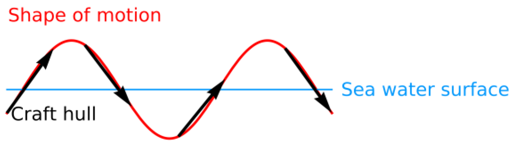
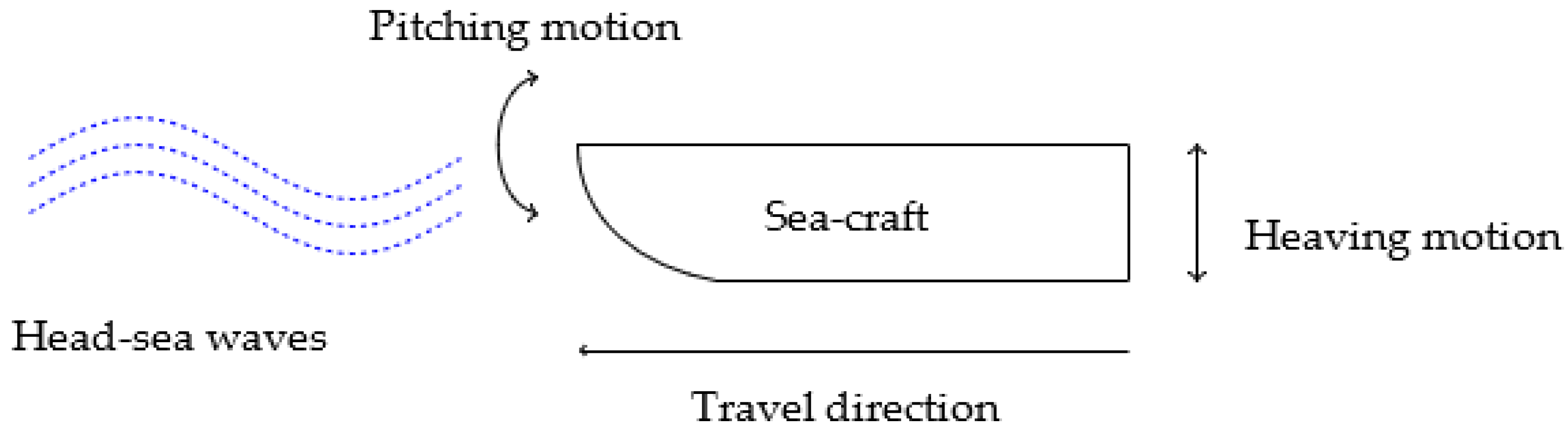
2.1. Heave and Pitch Equations of Motion
- is the component of the generalized mass matrix of the craft in the direction owing to the motion.
- is the added-mass coefficient in the direction due to the motion.
- is the damping coefficient in the direction due to the motion.
- is the hydrostatic restoring force coefficient in the direction due to the motion.
- is the complex amplitude of the exciting forces and moments in the direction.
- is the pitch coupling term coefficient.
- is the heave nonlinear term coefficient.
- is the heave coupling term coefficient.
- is the pitch nonlinear term coefficient.
- is the heave amplitude.
- and are the pitch amplitudes.
- is the natural frequency.
- is the external excitation frequency.
2.2. Amplitude Equations
- Heaving terms:
- Pitching terms:
- Heave:
- Pitch:
- Frequency of oscillations:
3. CFD Validation
3.1. The Viscous Model
3.2. The Computational Domain
3.2.1. Geometry
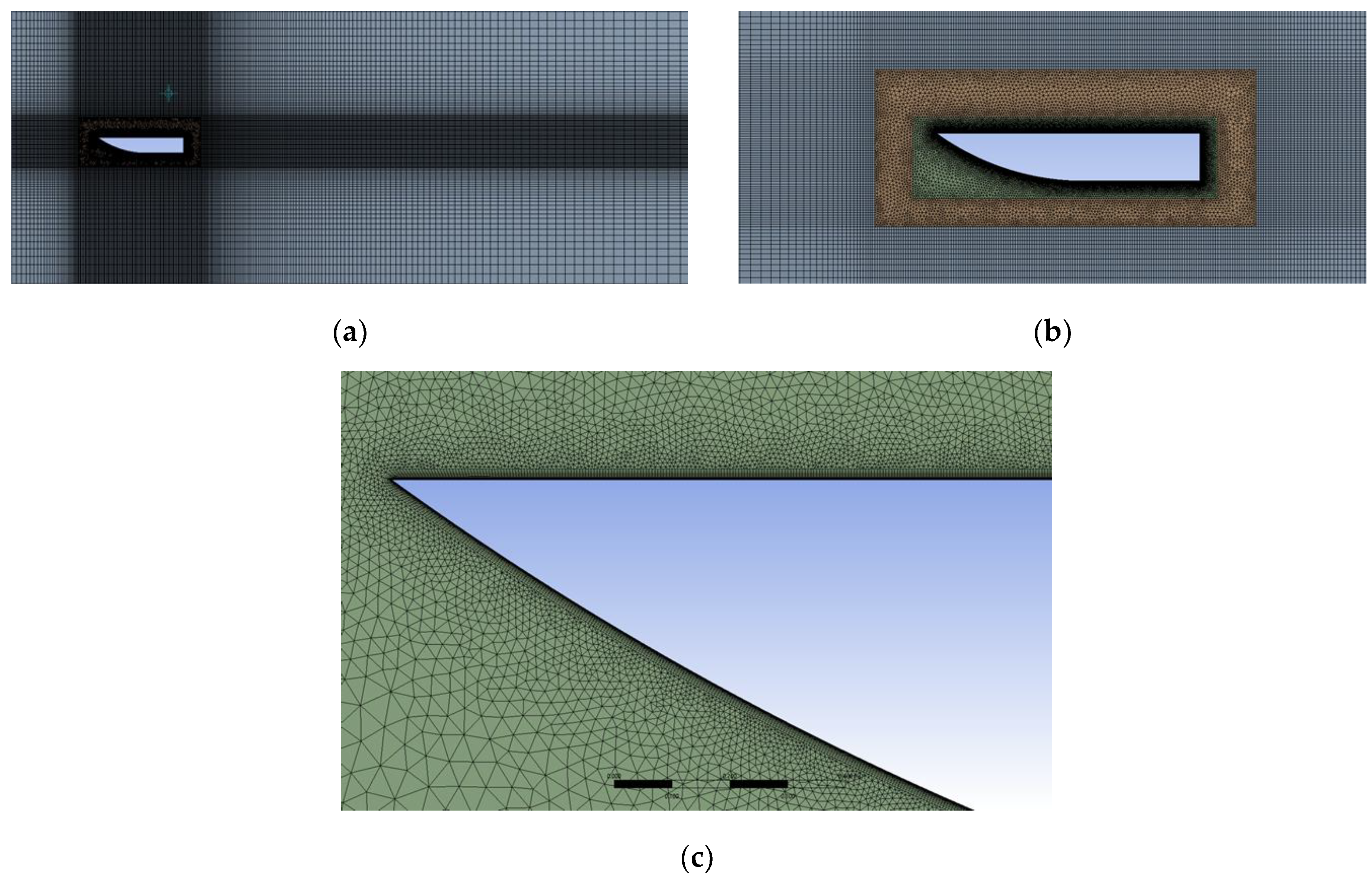
3.2.2. Mesh
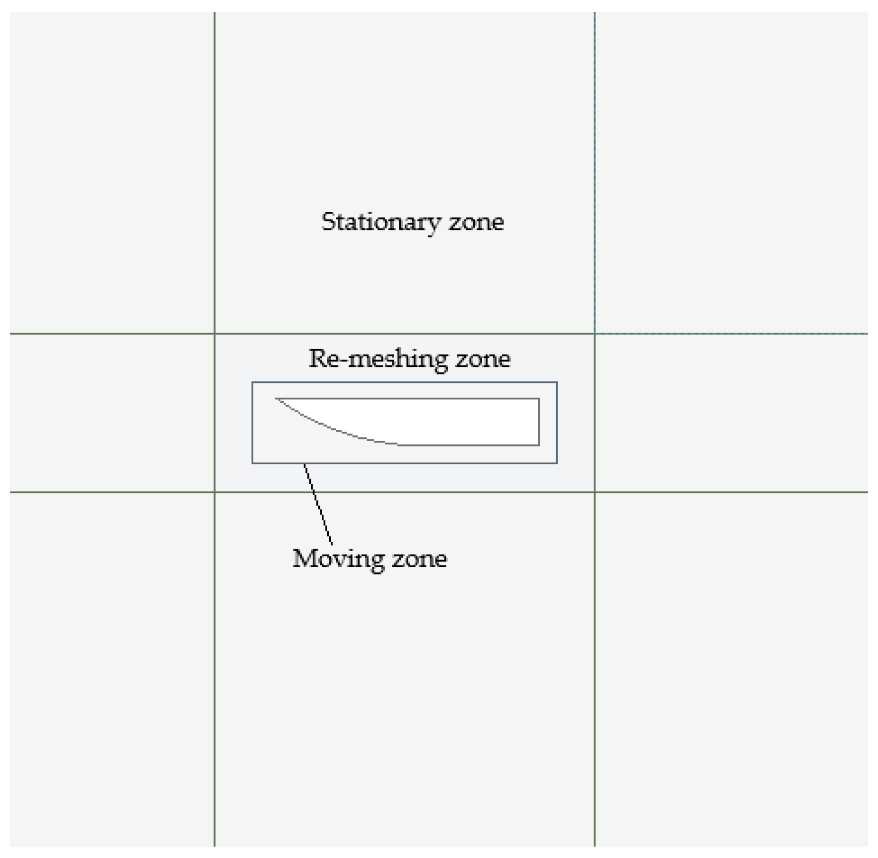
3.2.3. The Numerical Domain
4. Results
4.1. Hydrodynamic Coefficient Calculation
- The hull is divided into four sections to provide a representation of the underwater hull shape.
- The sectional added mass, damping, and restoring force coefficients are then determined by considering the hull as a series of transverse segments.
- Subsequently, the hydrodynamic coefficients of the heave and pitch equations are calculated by performing pressure integration along the length of the hull.
- Finally, the excitation forces and moments are calculated using Newton’s second law based on the given sea wave characteristics and hull shape.
4.2. Geometry and Conditions
4.3. Discussion of Results
4.4. Porpoising
5. Conclusions
Supplementary Materials
Author Contributions
Funding
Institutional Review Board Statement
Informed Consent Statement
Data Availability Statement
Conflicts of Interest
References
- Yun, L.; Bliault, A.; Doo, J. WIG Craft and Ekranoplan; Springer: Berlin/Heidelberg, Germany, 2010. [Google Scholar]
- Rozhdestvensky, K.V. Wing-in-Ground Effect Vehicles. Prog. Aerosp. Sci. 2006, 42, 211–283. [Google Scholar] [CrossRef]
- He, W.; Yu, P.; Li, L.K.B. Ground Effects on the Stability of Separated Flow Around a NACA 4415 Airfoil at Low Reynolds Numbers. Aerosp. Sci. Technol. 2018, 72, 63–76. [Google Scholar] [CrossRef]
- Faltinsen, O.M. Hydrodynamics of High-Speed Marine Vehicles; Cambridge University Press: Cambridge, UK, 2005. [Google Scholar]
- Duan, X.; Sun, W.; Chen, C.; Wei, M.; Yang, Y. Numerical Investigation of the Porpoising Motion of a Seaplane Planing on Water with High Speeds. Aerosp. Sci. Technol. 2019, 84, 980–994. [Google Scholar] [CrossRef]
- Nangia, R.K. Aerodynamic and Hydrodynamic Aspects of High-Speed Water Surface Craft. Aeronaut. J. 1987, 91, 241–268. [Google Scholar] [CrossRef]
- Dala, L. Dynamic Stability of a Seaplane in Takeoff. J. Aircr. 2015, 52, 964–971. [Google Scholar] [CrossRef]
- Jothimurugan, R.; Thamilmaran, K.; Rajasekar, S.; Sanjuán, M.A.F. Multiple Resonance and Antiresonance in Coupled Duffing Oscillators. Nonlinear Dyn. 2016, 83, 1803–1814. [Google Scholar] [CrossRef]
- Stosiak, M.; Karpenko, M.; Deptuła, A.; Urbanowicz, K.; Skačkauskas, P.; Deptuła, A.M.; Danilevičius, A.; Šukevičius, Š.; Łapka, M. Research of Vibration Effects on a Hydraulic Valve in the Pressure Pulsation Spectrum Analysis. J. Mar. Sci. Eng. 2023, 11, 301. [Google Scholar] [CrossRef]
- Lenci, S. Exact Solutions for Coupled Duffing Oscillators. Mech. Syst. Signal Process. 2022, 165, 108299. [Google Scholar] [CrossRef]
- Guo, Y.; Ma, D.; Yang, M.; Liu, X. Numerical Analysis of the Take-Off Performance of a Seaplane in Calm Water. Appl. Sci. 2021, 11, 6442. [Google Scholar] [CrossRef]
- Kring, D.; Huang, Y.-F.; Sclavounos, P.; Vada, T.; Braathen, A. Nonlinear Ship Motions and Wave-Induced Loads by a Rankine Method. In Twenty-First Symposium on Naval Hydrodynamics; The National Academies Press: Washington, DC, USA, 1997; pp. 45–63. [Google Scholar]
- Song, Z.; Deng, R.; Wu, T.; Duan, X.; Ren, H. Numerical Simulation of Planing Motion and Hydrodynamic Performance of a Seaplane in Calm Water and Waves. Eng. Appl. Comput. Fluid Mech. 2023, 17, 2244028. [Google Scholar] [CrossRef]
- Xie, H.; Wei, X.; Liu, X.; Liu, F. Analysis of Fluid Dynamic Behavior and Impact Load on Oblique Water Entry of a Two-Dimensional Seaplane Based on VOF Method. Ocean Eng. 2023, 274, 114028. [Google Scholar] [CrossRef]
- Tavakoli, S.; Zhang, M.; Kondratenko, A.A.; Hirdaris, S. A Review on the Hydrodynamics of Planing Hulls. Ocean Eng. 2024, 303, 117046. [Google Scholar] [CrossRef]
- Zhou, H.; Hu, K.; Mao, L.; Sun, M.; Cao, J. Research on Planing Motion and Stability of Amphibious Aircraft in Waves Based on Cartesian Grid Finite Difference Method. Ocean Eng. 2023, 272, 113848. [Google Scholar] [CrossRef]
- Wang, L.; Qin, S.; Fang, H.; Wu, D.; Huang, B.; Wu, R. Inhibition on Porpoising Instability of High-Speed Planing Vessel by Ventilated Cavity. Appl. Ocean Res. 2021, 111, 102688. [Google Scholar] [CrossRef]
- Zheng, Y.; Qu, Q.; Liu, P.; Wen, X.; Zhang, Z. Numerical Analysis of the Porpoising Motion of a Blended Wing Body Aircraft During Ditching. Aerosp. Sci. Technol. 2021, 119, 107131. [Google Scholar] [CrossRef]
- Zha, R.; Wang, K.; Sun, J.; Tu, H.; Hu, Q. Numerical Simulations of Seaplane Ditching on Calm Water and Uniform Water Current Coupled with Wind. J. Mar. Sci. Eng. 2024, 12, 296. [Google Scholar] [CrossRef]
- Morabito, M.G. A Review of Hydrodynamic Design Methods for Seaplanes. J. Ship Prod. Des. 2021, 37, 159–180. [Google Scholar] [CrossRef]
- Hwang, J.; Kim, M.; Lee, J. Longitudinal Static Stability Requirements for Wing in Ground Effect Vehicle. Int. J. Nav. Archit. Ocean Eng. 2015, 7, 508–517. [Google Scholar] [CrossRef]
- Collu, M.; Patel, S.; Trarieux, A. The Longitudinal Static Stability of an Aerodynamically Alleviated Marine Vehicle, A Mathematical Model. Proc. R. Soc. A 2010, 466, 2639–2656. [Google Scholar] [CrossRef]
- Huang, M.; Zhang, X.; Zhao, J.; Liu, L. The Water Impact Load Study for Seaplane During Get-Off and Alighting Process on Rough Water. J. Phys. Conf. Ser. 2022, 2282, 012024. [Google Scholar] [CrossRef]
- Lu, Y.; Deng, S.; Chen, Y.; Xiao, T.; Chen, J.; Liu, F.; Song, S.; Wu, B. Effects of Wave Parameters on Load Reduction Performance for Amphibious Aircraft with V-Hydrofoil. J. Aircr. 2024, 61, 1205–1217. [Google Scholar] [CrossRef]
- Chen, J.; Xiao, T.; Wang, M.; Lu, Y.; Tong, M. Numerical Study of Wave Effect on Aircraft Water-Landing Performance. Appl. Sci. 2022, 12, 2561. [Google Scholar] [CrossRef]
- Martin, M. Theoretical Prediction of Motions of High-Speed Planing Boats in Waves. J. Ship Res. 1978, 22, 140–169. [Google Scholar] [CrossRef]
- Xu, Y.; Luo, A.C.J. Series of Symmetric Period-1 Motions to Chaos in a Two-Degree-of-Freedom Van Der Pol-Duffing Oscillator. J. Vib. Test. Syst. Dyn. 2018, 2, 119–153. [Google Scholar] [CrossRef]
- Musielak, D.E.; Musielak, Z.E.; Benner, J.W. Chaos and Routes to Chaos in Coupled Duffing Oscillators with Multiple Degrees of Freedom. Chaos Solitons Fractals 2005, 24, 907–922. [Google Scholar] [CrossRef]
- Clementi, F.; Lenci, S.; Rega, G. 1:1 Internal Resonance in a Two DOF Complete System: A Comprehensive Analysis and Its Possible Exploitation for Design. Meccanica 2020, 55, 1309–1332. [Google Scholar] [CrossRef]
- Raj, S.P.; Rajasekar, S.; Murali, K. Coexisting Chaotic Attractors, Their Basin of Attractions, and Synchronization of Chaos in Two Coupled Duffing Oscillators. Phys. Lett. A 1999, 264, 283–288. [Google Scholar]
- Sunday, J. The Duffing Oscillator: Applications and Computational Simulations. Asian Res. J. Math. 2017, 2, 1–13. [Google Scholar] [CrossRef]
- Nayfeh, A.; Mook, D. Nonlinear Oscillations; John Wiley & Sons: Hoboken, NJ, USA, 1979. [Google Scholar]
- Bogolubov, N.; Mitropolski, Y. Asymptotic Methods in the Theory of Nonlinear Oscillations; Hindustan Publishing Corporation: New Delhi, Inida, 1961. [Google Scholar]
- El-Naggar, A.; Ismail, G. Analytical Solution of Strongly Nonlinear Duffing Oscillators. Alex. Eng. J. 2016, 55, 1581–1585. [Google Scholar] [CrossRef]
- Farzaneh, Y.; Tootoonchi, A.A. Analytical Solution of Strongly Nonlinear Duffing Oscillators. Comput. Math. Appl. 2010, 59, 2887–2895. [Google Scholar] [CrossRef]
- He, J. Variational Iteration Method—A Kind of Non-Linear Analytical Technique: Some Examples. Int. J. Non-Linear Mech. 1999, 34, 699–708. [Google Scholar] [CrossRef]
- Cveticanin, L. The Approximate Solving Methods for the Cubic Duffing Equation Based on the Jacobi Elliptic Functions. Int. J. Nonlinear Sci. Numer. Simul. 2009, 10, 1491–1516. [Google Scholar] [CrossRef]
- He, J.H. Homotopy Perturbation Method: A New Nonlinear Analytical Technique. Appl. Math. Comput. 2003, 135, 73–79. [Google Scholar] [CrossRef]
- Marinca, V.; Herisanu, N. Nonlinear Dynamical Systems in Engineering: Some Approximate Approaches; Springer Science & Business Media: Berlin/Heidelberg, Germany, 2012. [Google Scholar]
- Nayfeh, A.H. Perturbation Methods; John Wiley & Sons: Hoboken, NJ, USA, 2008. [Google Scholar]
- Drazin, P.G. Nonlinear Systems; Cambridge University Press: Cambridge, UK, 1992. [Google Scholar]
- Nayfeh, A.H. Introduction to Perturbation Techniques; John Wiley & Sons: Hoboken, NJ, USA, 2011. [Google Scholar]
- Murdock, J.A. Perturbations: Theory and Methods; SIAM: Philadelphia, PA, USA, 1999. [Google Scholar]
- Holmes, M.H. Introduction to Perturbation Methods; Springer Science & Business Media: Berlin/Heidelberg, Germany, 2012. [Google Scholar]
- Bhattacharyya, R. Dynamics of Marine Vehicles; John Wiley & Sons Incorporated: Hoboken, NJ, USA, 1978. [Google Scholar]
- Li, X.; Zhang, L.; Zhang, H.; Li, K. Singularity Analysis of Response Bifurcation for a Coupled Pitch–Roll Ship Model with Quadratic and Cubic Nonlinearity. Nonlinear Dyn. 2019, 95, 2659–2674. [Google Scholar] [CrossRef]
- Javanmardi, N.; Ghadimi, P. Hydroelastic Analysis of a Semi-Submerged Propeller Using Simultaneous Solution of Reynolds-Averaged Navier–Stokes Equations and Linear Elasticity Equations. Proc. Inst. Mech. Eng. Part M 2018, 232, 199–211. [Google Scholar] [CrossRef]
- Özdemir, Y.H.; Barlas, B. Numerical Study of Ship Motions and Added Resistance in Regular Incident Waves of KVLCC2 Model. Int. J. Nav. Archit. Ocean Eng. 2017, 9, 149–159. [Google Scholar] [CrossRef]
- Hellsten, A. Some Improvements in Menter’s k-ω SST Turbulence Model. In Proceedings of the 29th AIAA Fluid Dynamics Conference, Albuquerque, NM, USA, 15–18 June 1998; p. 2554. [Google Scholar]
- Korvin-Kroukovsky, B.V. Investigation of Ship Motions in Regular Waves. In SNAME Transactions; Stevens Institute of Technology, Experimental Towing Tank: Hoboken, NJ, USA, 1955. [Google Scholar]
- Niklas, K.; Pruszko, H. Full-Scale CFD Simulations for the Determination of Ship Resistance as a Rational, Alternative Method to Towing Tank Experiments. Ocean Eng. 2019, 190, 106435. [Google Scholar] [CrossRef]
- Wang, Z.; Stern, F. Moving Air-Water Interface on No-Slip Solid Walls for High-Speed Planing Hulls. Ships Offshore Struct. 2024, 1, 1–8. [Google Scholar] [CrossRef]
- Masri, J.; Dala, L.; Huard, B. A Review of the Analytical Methods Used for Seaplanes’ Performance Prediction. Aircr. Eng. Aerosp. Technol. 2019, 91, 820–833. [Google Scholar] [CrossRef]
- Salvesen, N.; Tuck, E.O.; Faltinsen, O. Ship Motions and Sea Loads. Trans. Soc. Nav. Archit. Mar. Eng. 1970, 78, 250–287. [Google Scholar]
- Lewis, E.V. Principles of Naval Architecture, 3rd ed.; Society of Naval Architects and Marine Engineers: Jersey City, NJ, USA, 1989. [Google Scholar]
- Fossen, T.I. Handbook of Marine Craft Hydrodynamics and Motion Control; John Wiley & Sons: Hoboken, NJ, USA, 2011. [Google Scholar]
- Zhen, Y.; Chen, J. Rogue Waves on the Periodic Background in the High-Order Discrete MKdV Equation. Nonlinear Dyn. 2023, 111, 12511–12524. [Google Scholar] [CrossRef]
- Liu, J.; Hayatdavoodi, M.; Ertekin, R.C. A Comparative Study on Generation and Propagation of Nonlinear Waves in Shallow Waters. J. Mar. Sci. Eng. 2023, 11, 917. [Google Scholar] [CrossRef]
- Fu, C.; Wang, J.; Zhao, T. Analytical Calculation of Instantaneous Liquefaction of a Seabed Around Buried Pipelines Induced by Cnoidal Waves. J. Mar. Sci. Eng. 2023, 11, 1319. [Google Scholar] [CrossRef]
- Gao, X.; Ma, X.; Li, P.; Yuan, F.; Wu, Y.; Dong, G. Nonlinear Analytical Solution for Radiation Stress of Higher-Order Stokes Waves on a Flat Bottom. Ocean Eng. 2023, 286, 115622. [Google Scholar] [CrossRef]
- Pambela, A.R.; Ma, C.; Maeda, T.; Iijima, K. Stokes Wave Traveling Along a Thin Elastic Plate Floating at Water Surface. J. Fluids Struct. 2023, 120, 103919. [Google Scholar] [CrossRef]
- Gao, Z.; Shi, Z. Numerical Study on Damaged Ship Rolling and Capsizing in Irregular Beam Waves During Quasi-Steady Flooding. Ocean Eng. 2023, 289, 116308. [Google Scholar] [CrossRef]
- Krata, P.; Gil, M.; Hinz, T.; Koziol, P. A Multiparameter Simulation-Driven Analysis of Ship Response When Turning Concerning a Required Number of Irregular Wave Realizations. Ocean Eng. 2024, 302, 117701. [Google Scholar] [CrossRef]


| Parameter | Model 1 | Model 2 |
|---|---|---|
| Overall length (ft) | 19.2 | 5 |
| Beam length (ft) | 2.592 | 0.666 |
| Draft (ft) | 1.144 | 0.081 |
| Weight (lb) | 2838 | 33.2 |
| Radius of gyration (ft) | 4.588 | 1.25 |
| Moment of inertia (lb.sec2.ft) | 1780.2 | 1.611 |
Disclaimer/Publisher’s Note: The statements, opinions and data contained in all publications are solely those of the individual author(s) and contributor(s) and not of MDPI and/or the editor(s). MDPI and/or the editor(s) disclaim responsibility for any injury to people or property resulting from any ideas, methods, instructions or products referred to in the content. |
© 2024 by the authors. Licensee MDPI, Basel, Switzerland. This article is an open access article distributed under the terms and conditions of the Creative Commons Attribution (CC BY) license (https://creativecommons.org/licenses/by/4.0/).
Share and Cite
Masri, J.; Dala, L.; Huard, B. Nonlinear Dynamic Stability Analysis of Ground Effect Vehicles in Waves Using Poincaré–Lindstedt Perturbation Method. J. Mar. Sci. Eng. 2024, 12, 2154. https://doi.org/10.3390/jmse12122154
Masri J, Dala L, Huard B. Nonlinear Dynamic Stability Analysis of Ground Effect Vehicles in Waves Using Poincaré–Lindstedt Perturbation Method. Journal of Marine Science and Engineering. 2024; 12(12):2154. https://doi.org/10.3390/jmse12122154
Chicago/Turabian StyleMasri, Jafar, Laurent Dala, and Benoit Huard. 2024. "Nonlinear Dynamic Stability Analysis of Ground Effect Vehicles in Waves Using Poincaré–Lindstedt Perturbation Method" Journal of Marine Science and Engineering 12, no. 12: 2154. https://doi.org/10.3390/jmse12122154
APA StyleMasri, J., Dala, L., & Huard, B. (2024). Nonlinear Dynamic Stability Analysis of Ground Effect Vehicles in Waves Using Poincaré–Lindstedt Perturbation Method. Journal of Marine Science and Engineering, 12(12), 2154. https://doi.org/10.3390/jmse12122154