Doppler Compensation Techniques for M-Ary Sequence Spread Spectrum Signals Based on Correlation Cost Factors in Mobile Underwater Acoustic Communication

Abstract

Unlike terrestrial radio, the speed of sound in the ocean is relatively slow, which results in mobile underwater M-ary spread spectrum communication typically exhibiting significant and variable multipath effects along with strong Doppler effects, leading to rapid carrier phase shifts in the received signal that severely impact decoding accuracy. This study aims to address the issue of rapid carrier phase shifts caused by significant time-varying Doppler shifts during mobile underwater M-SS communication. This paper innovatively proposes a method for updating matched filters based on correlation cost factors. By calculating the correlation cost factors for each received symbol, the method guides the direction of Doppler estimation and updates the matched filters. After identifying the optimal match, the received symbols are shifted, correlated, and decoded. Simulation and sea trial results indicate that this method demonstrates higher computational efficiency and improved decoding accuracy compared to traditional Doppler estimation matched filters under low signal-to-noise ratio conditions, and exhibits greater robustness under complex motion conditions.

1. Introduction

It is well known that the underwater acoustic channel is one of the most intricate wireless communication channels, particularly under conditions of low signal-to-noise ratio (SNR) and pronounced Doppler effects. In order to address the challenges posed by low SNR and to achieve robust underwater acoustic communication, extensive research efforts have been undertaken [1,2,3,4]. Among the various underwater acoustic communication technologies, Direct Sequence Spread Spectrum (DSSS) is a commonly employed communication technique due to its exceptional interference resistance and robustness against channel fading. DSSS expands the signal over a broader frequency band by utilizing noise-like pseudo-random spreading codes (SCs), enabling coherent demodulation systems to recover the signal through coherent despreading of energy [5]. Generally, the spreading gain is substantial (for instance, when the SC length is 511, the spreading gain reaches 27 dB) [6]. This gain facilitates the accurate decoding of received signals under noisy conditions while also providing a degree of confidentiality. However, the communication rate of DSSS is constrained by the narrow bandwidth of the underwater acoustic channel, resulting in a relatively low transmission speed [7,8]. Furthermore, due to the time-varying nature of the marine environment, the Doppler shift within a single frame often exhibits variability, with longer transmission packets facing even more pronounced Doppler shifts. The time-varying Doppler shift can induce rapid fluctuations in the carrier phase, significantly diminishing the spreading gain during the coherent despreading process. In the context of time-varying Doppler shifts, the robustness of underwater spread spectrum communication is considerably compromised. Therefore, enhancing the communication rate of underwater spread spectrum communication and mitigating time-varying Doppler shifts are two critical research focal points in this field.

To enhance the communication rate of spread spectrum communication, a Code Index Modulation-Spread Spectrum (CIM-SS) scheme has been proposed in the realm of terrestrial radio communication [9]. By introducing the spreading code domain and employing a new dimension to map information bits, the data rate is enhanced. This scheme preserves the advantages of spread spectrum modulation without increasing the system’s computational complexity and is easy to implement. The study in [10] extended the CIM technology. Simulation results indicate that, compared to traditional DSSS systems, the proposed modulation scheme exhibits superior performance in terms of data rate, energy consumption, and complexity.

To address the time-varying Doppler effect, which induces rapid carrier phase shifts and reduces spreading gain, Doppler estimation and compensation are generally required. In previous studies, the methods for Doppler estimation can be categorized as follows: (1) utilizing adjacent pseudo-random codes for time-domain correlation to compute Doppler factors; (2) employing Doppler-sensitive training sequences to conduct time-frequency two-dimensional search methods; (3) utilizing LFM signals to perform block estimation methods; (4) combining coding techniques with iterative estimation algorithms. Among these, the method of using adjacent pseudo-random codes for time-domain correlation to estimate Doppler factors can obtain Doppler estimates between adjacent symbols, but it requires adjacent symbols to have the same pseudo-random code, making it applicable only to DSSS processing with relatively low spectral efficiency [7,11]. Hu et al. designed an M-ary sequence spread spectrum (M-SS) communication method that incorporates several identical pseudo-random codes into the frame structure for Doppler estimation. Although it sacrifices some communication rate, the accuracy of Doppler estimation is significantly improved [12,13]. The block estimation method using LFM signals can only calculate the average Doppler within a single frame and is not suitable for long frame sequences [14]. Furthermore, coding iterative techniques require a high signal-to-noise ratio, rendering them unsuitable for underwater acoustic communication under low SNR ratio conditions [15,16]. L. Freitag et al. proposed a receiver based on the Minimum Mean Square Error (MMSE) criterion for the acquisition of Direct Sequence Spread Spectrum (DSSS) signals. The core method involves using an adaptive Decision Feedback Equalizer (DFE) in combination with spreading codes for synchronization and tracking. This approach is particularly suitable for complex multipath propagation environments in multi-user underwater acoustic communications [17]. J. Neasham et al. analyzed the sea trial results of the Phorcys V0 underwater acoustic communication waveform, validating its performance across multiple frequency bands and complex channel environments, and evaluated the performance of different receiver structures [18]. Kwang B. Yoo et al. proposed a method based on the measurement and updating of passive matched filters to enhance spreading gain by mitigating variable multipath effects and performing Doppler estimation within symbols; however, the calculation speed and efficiency of Doppler estimation significantly decreased under low SNR ratios [5]. Sun et al. introduced a novel linear prediction equation suitable for sparse underwater acoustic channels, calculating linear prediction coefficients by estimating the Doppler frequency shift for each symbol. However, the computational load and prediction accuracy are significantly influenced by the signal-to-noise ratio, and the algorithm exhibits high complexity [19]. Due to the relatively low speed of sound in the ocean, even minor velocity changes in underwater platforms can induce substantial Doppler frequency shifts. Methods for Doppler estimation in underwater acoustic communication primarily involve estimating and predicting the velocity of movement, which entails significant computational load and complexity. When there are deviations in velocity estimation, the Doppler estimation is also significantly affected and constrained by the accuracy of the estimation. During the process of Doppler compensation, it is common to perform a search within a certain range of the Doppler estimation results before updating them into the matched filter bank, a process referred to as Doppler precise estimation. Thus, even if there is a certain deviation in Doppler estimation, it will not significantly impact the spreading gain; the permissible range of deviation in Doppler estimation is referred to as Doppler-tolerant [16].

Influenced by the studies in [9,10], this research introduces the CIM-SS technology from the field of radio communication into the realm of underwater acoustic communication, innovatively designing an M-SS communication transmission module based on polarity and spreading code index modulation, which partitions the transmitted information into polarity data and index data for separate modulation, achieving a transmission rate that is $lo{g}_2(M+n)$ times higher than that of a DSSS communication system transmission module with the same signal length, where M denotes the size of the spreading code index library and n represents the number of transmitted symbols, thereby further enhancing spectral efficiency.

In response to the issue of carrier frequency offset (CFO) caused by time-varying Doppler frequency shifts in complex channel environments, this paper focuses on enhancing Doppler-tolerant, traditional methods typically involve conducting a search within a certain range of the Doppler estimation results, followed by performing correlation-matched filtering based on the various search values and selecting the search position corresponding to the highest output peak as the final Doppler estimation result. This method is feasible for DSSS, but it introduces certain errors in the final estimation results when applied to M-SS communication, as the process of M-SS despreading requires not only inputting the signal into the Doppler precise estimator but also into the spreading code index library, resulting in a two-dimensional correlation peak matrix composed of the search frequency shift dimension and the spreading code index dimension. Previous studies typically assumed that the frequency shift position corresponding to the highest peak in the matrix should be selected as the Doppler estimation result, but this approach is not rigorous for M-SS communication, as the correlation between spreading codes has been disrupted under conditions of pronounced channel time variability, and at the searched frequency shift positions, it is possible for peaks at positions with larger errors to exceed those at positions with smaller errors. Although the corresponding index decoding position may be correct, the accumulation of errors can still lead to subsequent decoding inaccuracies.

To address the aforementioned issues, we propose a method for updating matched filters based on correlation cost factors for M-SS communication. By calculating the correlation cost factors, the accuracy of Doppler estimation for each symbol can be assessed, which allows for guiding the direction of Doppler estimation for subsequent symbols in subsequent processing, thereby preventing excessive accumulation of estimation errors. Through simulations and sea trials, the reception method utilizing correlation cost factor-based updates to matched filters significantly outperforms traditional reception methods in various aspects.

The remainder of this paper is organized as follows. Section 2 describes the newly proposed M-ary spread spectrum communication transmission module, the conventional reception method for M-SS, and the theoretical aspects of the reception method based on correlation cost factor updates to matched filters; Section 3 presents numerical simulation studies, including parameter settings and decoding performance tests under various mobility conditions; Section 4 analyzes data from sea trial experiments; Section 5 provides a summary of the entire paper.

2. Communication System Model and Theory

In this section, we provide an explanation and theoretical derivation of the communication system composed of the previously proposed transmitter and receiver, as well as the Doppler estimation process involved in signal processing.

2.1. Transmitter and Underwater Acoustic Channel Transmission Process

Without loss of generality, this section uses BPSK as an example. The detailed steps of the transmitter are illustrated in Figure 1, where the binary bit stream data at the transmitter are divided into polarity data $a\left[0\right]$ and index data $a[n-1]$, and further segmented into i groups corresponding to the data streams $a_1\left[0\right]$$a_2\left[0\right]\dots a_i\left[0\right]$ and $a_1[n-1]$$a_2[n-1]\dots a_i[n-1]$, where n denotes the number of bits in each group, and its value is related to the size of the SS code index library, corresponding to $M=2^{n-1}$, where M represents the number of entries in the SS code index library. First, the $i\times (n-1)$ index data $a_i[n-1]$ are converted into decimal data $b_i(1\le b_i\le M)$ and the corresponding PN code $c_{i,b_i}\left(t\right)$ is selected from the SS code index library as the SS code for spreading, based on the position of $b_i$ in the SS code index table, the activated PN code $c_{i,b_i}\left(t\right)$ is represented as follows:

$$c_{i,b_i}\left(t\right)=\sum _{m=0}^{L-1}{c}_{i,b_i,m}{g}_c(t-m{T}_c)$$

(1)

$$g_c(t-m{T}_c)=\left\{\begin{array}{cc}1,\hfill & \le t\le T_c\hfill \\ 0,\hfill & \mathrm{otherwise}\hfill \end{array}\right.$$

(2)

where L represents the length of the activated PN code, $T_c$ denotes the chip duration, $c_{i,b_i}=[c_{1,b_1}{c}_{2,b_2}...c_{i,b_i}]$ represents the sequence of the active code. The transmitted data $x\left(t\right)$ after merging with the polarity data can be expressed as follows:

$$x\left(t\right)=\sum _{i=1}^{\infty }{a}_i\left[0\right]c_{i,b_i}\left(t\right)$$

(3)

The transmitted data $x\left(t\right)$ pass through a pulse-shaping filter prior to modulation, and the baseband signal $\tilde{s}\left(t\right)$ can be expressed as follows:

$$\tilde{s}\left(t\right)=\sum _{i=0}^{\infty }x\left(t\right)\omega (t-i{T}_s)$$

(4)

Here, $T_s$ represents the symbol interval, $\omega \left(t\right)$ is the pulse-shaping function, and $\beta$ denotes the roll-off factor. The transmitted signal, suitable for underwater acoustic channels after carrier modulation, can be expressed as follows:

$$s\left(t\right)=\sum _{i=0}^{\infty }\tilde{s}\left(t\right)e^{j2\pi f_{c}t}$$

(5)

where $f_c$ is a carrier center frequency.

It is well-known that the underwater acoustic (UWA) channel is a typical double-diffusion channel [20,21]. The impulse response $h_i(t,\tau )$ of the time-varying channel for the i-th symbol in the transmitted data can be expressed as follows [22,23]:

$$h_i(t,\tau )=\sum _{q=0}^{Q-1}{A}_{q,i}\left(t\right)\delta (\tau -{\tau }_{q,i}\left(t\right))$$

(6)

Here, Q denotes the number of channel taps, while the amplitude and delay of the q-th path for the i-th symbol can be represented as $A_{q,i}\left(t\right)$ and ${\tau }_{q,i}\left(t\right)$.

Ultimately, the received signal $r\left(t\right)$ can be described as the convolution of the transmitted signal and the channel impulse response, and its final expression is as follows:

$$\begin{array}{cc}\hfill r\left(t\right)& =\Re \left\{\sum _{i=1}^{\infty }\sum _{q=0}^{Q-1}{A}_{q,i}\left(t\right)a_i\left[0\right]c_{i,b_i}\omega e^{j2\pi f_c(t-{\tau }_{q,i}\left(t\right))}\right\}+\eta \left(t\right)\hfill \end{array}$$

(7)

where $\eta \left(t\right)$ is the noise in the transmission process, $c_{i,b_i}=c_{i,b_i}(t-{\tau }_{q,i}\left(t\right))-i{T}_s)$, $\omega =\omega (t-{\tau }_{q,i}\left(t\right)-i{T}_s)$.

2.2. Conventional Reception Method for M-SS

After performing synchronization, filtering, and other preprocessing on the received signal, Doppler estimation is also required. This paper conducts both coarse and fine Doppler estimation on the received signal [24]. When the estimated frequency shift value after coarse Doppler estimation significantly deviates from the actual frequency shift value, the correlation of the spread spectrum symbols will be markedly reduced. In this case, it is essential to perform a Doppler frequency shift search within a certain range based on the coarse estimation to restore correlation; this process is defined as fine Doppler estimation. As shown in Figure 2, the preprocessed signal is passed through the coarse Doppler estimator to obtain the initially estimated frequency shift value, which serves as the initial search value for subsequent fine Doppler estimation, and the signal is then input into the fine Doppler estimator. First, the signal is input into multiple locally generated correlators for frequency shift searching. Given that the modulation scheme employed in this paper is M-SS spreading, the signal must also be input into the spreading code index library for correlation analysis, ultimately resulting in a correlation matrix composed of the carrier frequency offset (CFO) and the spreading code index dimensions, from which the corresponding frequency shift and index decoding values are selected based on the matrix peak, thereby obtaining the Doppler coefficient for the symbol (the detailed theoretical derivation of the estimation process is presented in reference [16]). However, the computational load of the search process is substantial; thus, we prefer a more accurate coarse Doppler estimation to reduce the search range. Numerous studies have been conducted on this aspect (see reference [19,25,26,27]), primarily focusing on velocity prediction and interpolation methods, which often exhibit limited adaptability to complex motion states, and many methods are only applicable to direct sequence spread spectrum communication, rendering them unsuitable for M-ary spread spectrum communication. To address the issues of reduced correlation of spread spectrum symbols resulting from inaccurate coarse Doppler estimation during communication under complex motion states, as well as the computational efficiency of subsequent fine Doppler estimation, we propose a reception method correlation cost factor-based updates to matched filters for M-SS (CCF-MSS), focusing on enhancing Doppler tolerance.

2.3. Correlation Cost Factor-Based Updates to Matched Filters Reception Method for M-SS (CCF-MSS)

When the channel exhibits strong time variability and low SNR, many velocity prediction methods often yield suboptimal results, which is attributed to the significant reduction in the overall correlation of the time-varying channel. It has been demonstrated that even with rapid time variation in the channel, the channel correlation of consecutive symbols remains relatively high [25,28], which also indicates that the frequency shifts of consecutive symbols are similarly close; we can utilize the accurate estimation results of preceding symbols to guide the frequency shift estimation direction of subsequent symbols. Here, we consider two methods for selecting frequency shift estimation results: The first method involves selecting the frequency shift estimation results based on the matrix peaks of the two-dimensional correlation matrix mentioned in Section 2.2. The second method involves selecting the frequency shift estimation results based on the correlation cost factors calculated from the two-dimensional correlation matrix. This second method represents an innovative approach that we propose, which will be introduced and theoretically derived in the following sections. The signal processing flow of the proposed method is illustrated in the reception section of Figure 1. The received signal is first synchronized and then input into the “Doppler Coarse Estimation” module to preliminarily estimate the Doppler value of the first symbol. Subsequently, the estimation result is passed to the “Matched Filter” module for fine Doppler estimation and computation of the correlation cost factor. Based on the outcome of the correlation cost factor, the final decoding result is output, and the current Carrier Frequency Offset (CFO) value is saved to feed back into the “Matched Filter” module as an initial reference point for the Doppler search of the next symbol. As illustrated in Figure 1, the computational efficiency of CCF-MSS does not show a marked improvement over WDE-MSS or CDE-MSS, primarily because WDE-MSS and CDE-MSS do not involve precise Doppler estimation, a process that demands substantial computational resources. When juxtaposed with FDE-MSS under identical search iterations, CCF-MSS merely necessitates an additional division operation, which accounts for a negligible computational load. Consequently, it can be inferred that FDE-MSS and CCF-MSS exhibit similar computational demands given the same number of searches. Nevertheless, CCF-MSS distinguishes itself by calculating a correlation cost factor during the search process; should this factor fall below a predetermined threshold, the search can be prematurely terminated. This capability allows for significant reductions in computational effort compared to the conventional fixed-iteration FDE-MSS, and it also enhances the accuracy of the decoding results.

We first designed a specialized frame structure, as illustrated in Figure 3, in which the first two symbols of each frame are assigned the same spreading code, referred to as the repeated code group, to facilitate Doppler estimation. Although this may slightly reduce the transmission rate, it allows for a more accurate initial Doppler estimation. After performing preprocessing operations such as synchronization and filtering on the received signal, the first repeated code group in the signal is subjected to coarse Doppler estimation on a frame-by-frame basis, yielding the initially estimated carrier frequency ${f_c}^{\ast }$ followed by searching for frequency shifts with a precision of $df$ and a range of $2k$ for the carrier frequency, which generates a two-dimensional correlation matrix, and after calculating the correlation cost factors at each point in the matrix, outputs the index positions and de-spreading results. Subsequently, the matching filters are updated based on the correlation cost factors. The following sections will discuss the process of coarse Doppler estimation, the calculation methods for correlation cost factors, and the theoretical derivation of the receiver decoding process.

2.3.1. Coarse Doppler Estimation

Given that the duration of the spreading code in this paper is relatively short, it is reasonable to approximate the Doppler factor as invariant within the time width of a single spreading code. From Section 2.1, the time-domain waveforms of the adjacent repeated codes are $c_{1,b_1}\left(t\right)$ and $c_{2,b_2}\left(t\right)$, where $b_1$ and $b_2$ are equal, and the Doppler factors for the adjacent spreading codes are ${\beta }_1$ and ${\beta }_2$; the corresponding received signal after down-conversion to baseband can be expressed as follows:

$$r_{symbol1}=a_1\left[0\right]c_{1,b_1}\left((1+{\beta }_1)t\right)e^{j2\pi f_{c}t}$$

(8)

$$r_{symbol2}=a_2\left[0\right]c_{2,b_2}((1+{\beta }_2)t+{\displaystyle \frac{L{\beta }_1}{1+{\beta }_{1}B}})e^{j2\pi f_{c}t}$$

(9)

Here, L denotes the length of a spreading symbol and ${\displaystyle \frac{L{\beta }_1}{1+{\beta }_{1}B}}$ represents the compression and expansion interference experienced by the second symbol due to the first symbol. Taking the absolute value of the correlation of the conjugates of $r_{symbol1}$ and $r_{symbol1}$ yields

$$\begin{array}{cc}\hfill R& =\int r_{symbol1}(t+\tau )r_{symbol2}^{\ast }\left(t\right)dt\hfill \\ \hfill & =|\int c_{1,b_1}\left((1+{\beta }_1)(t+\tau )\right)c_{2,b_2}((1+{\beta }_2)t+{\displaystyle \frac{L{\beta }_1}{(1+{\beta }_1)B}})dt|\hfill \end{array}$$

(10)

Here, let $t^{\ast }=(1+{\beta }_2)t+{\displaystyle \frac{L{\beta }_1}{(1+{\beta }_1)B}}$ substituting this yields

$$R=|\int c_{1,b_1}({\displaystyle \frac{1+{\beta }_1}{1+{\beta }_2}}{t}^{\ast }-{\displaystyle \frac{L{\beta }_1}{(1+{\beta }_2)B}}+(1+{\beta }_1)\tau )c_{2,b_2}\left(t^{\ast }\right)dt|$$

(11)

Since the changes in Doppler factors between adjacent spreading symbols are minimal, it can be assumed that ${\displaystyle \frac{1+{\beta }_1}{1+{\beta }_2}}\approx 1$. Therefore, when R exhibits a correlation peak, $\tau ={\displaystyle \frac{L{\beta }_1}{(1+{\beta }_1)(1+{\beta }_2)B}}\approx {\displaystyle \frac{L{\beta }_1}{{(1+{\beta }_1)}^{2}B}}$ thus ${\beta }_1={\displaystyle \frac{L-2B\tau +\sqrt{L^2-2B\tau L}}{2B\tau }}$, and when $\tau =0$, ${\beta }_1$ is also equal to 0. Consequently, the Doppler factor can be initially calculated based on the repeated code group, which serves as an initial value for subsequent fine Doppler estimation. It is worth noting that this method entails a certain computational load, and may lead to a reduction in communication rate. However, in this paper, each frame utilizes only one pair of repeated code groups for Doppler estimation, and subsequent processing relies on the correlation cost factors for fine Doppler estimation, thus having a negligible impact on the overall computational load and communication rate.

2.3.2. Correlation Cost Factors

The correlation cost factor is defined as the ratio of the second-largest correlation peak to the maximum correlation peak at each frequency shift search position within the two-dimensional correlation matrix formed by the carrier frequency offset (CFO) and the spreading code index. During the despreading process, the greater the difference between the maximum correlation peak and the other correlation peaks, the more accurate the despreading result. Based on the correlation cost factor, we can assess the accuracy of the despreading process, and subsequently adjust the direction of Doppler compensation for the following symbols. The correlation cost factor is expressed as follows:

$$G_i={\displaystyle \frac{R_{se{c}_{k\times n}}}{R_{ma{x}_{k\times n}}}},sebjecttok=0\pm 1\pm 2,...$$

(12)

where $G_i$ is the correlation cost factor, $R_{sec}$ is the second largest correlation peak, $R_{max}$ is the largest correlation peak, k is the number of search steps, and n is the number of PN codes.

2.3.3. Theoretical Derivation of the Receiver Decoding Process

The following presents the theoretical derivation of the decoding process for the i-th. The frequency offset value output after evaluating the correlation cost factor is denoted as $f_{c_{est},i}=f_{c_{est},i-1}+{k_i}^{\ast }·df$. Here, i denotes the i-th symbol (where i ≥ 2), $f_{c_{est},i-1}={f_c}^{\ast }+{\sum }_{i=2}^i{k_{i-1}}^{\ast }·df$, $f_{c_{est},i-1}$ representing the CFO value transmitted from the $(i-1)$-th, $k_{i-1}^{\ast }·df$ is the selected CFO value during the compensation process for the i-th symbol. Next, we employ a non-coherent demodulation method. First, two local carrier signals are generated at the receiver, $y_c=\Re \left\{\begin{array}{c}{e}^{j2\pi f_{c}t}\hfill \end{array}\right\}$ and $y_s=\Im \left\{\begin{array}{c}{e}^{j2\pi f_{c}t}\hfill \end{array}\right\}$, which are then used to down-convert the received signal, followed by passing through a low-pass filter (LPF):

$$\begin{array}{cc}\hfill {\tilde{r}}_c\left(t\right)& =LPF(r\left(t\right)\Re \left\{e^{j2\pi f_{c_{est},i}t}\right\})\hfill \\ \hfill & ={\displaystyle \frac{1}{2}}\Re \left\{\sum _{i=1}^{\infty }\sum _{q=0}^{Q-1}{A}_{q,i}\left(t\right)a_i\left[0\right]c_{i,b_i}{e}^{j{\varphi }_{q,i}\left(t\right)}\right\}+w\left(t\right)\hfill \end{array}$$

(13)

Here, the carrier phase shift ${\varphi }_{q,i}\left(t\right)=2\pi (f_{c_{est},i}t-f_c{\tau }_{q,i}\left(t\right))$. This includes the time-varying phase of the q-th path, where $w\left(t\right)$ represents the baseband noise. When the dominant Doppler shift is caused by large-scale movement of the receiver, it can be assumed that for a single symbol, all paths have equal Doppler factors [29], and thus ${\tau }_{q,i}\left(t\right)={\tau }_i\left(t\right)$${\varphi }_{q,i}\left(t\right)={\varphi }_i\left(t\right)$$q=[0,Q-1]$. In this paper, considering the underwater acoustic communication process under the conditions of low SNR and significant time-varying Doppler shifts, the energy of the main path is significantly greater than that of other paths; therefore, the energy of other paths is treated as noise in this study, and after normalizing the impulse response amplitude of the main path, we have the following:

$$\begin{array}{cc}\hfill {\tilde{r}}_c\left(t\right)& =\Re \left\{\sum _{i=1}^{\infty }{a}_i\left[0\right]c_{i,b_i}(t-{\tau }_i\left(t\right)-i{T}_s)e^{j{\varphi }_i\left(t\right)}\right\}+w\left(t\right)\hfill \\ \hfill & =\sum _{i=1}^{\infty }{a}_i\left[0\right]c_{i,b_i}(t-{\tau }_i\left(t\right)-i{T}_s)cos\left({\varphi }_i\left(t\right)\right)+w\left(t\right)\hfill \end{array}$$

(14)

Similarly, the signal from the other path is as follows:

$${\tilde{r}}_s\left(t\right)=\sum _{i=1}^{\infty }{a}_i\left[0\right]c_{i,b_i}(t-{\tau }_i\left(t\right)-i{T}_s)sin\left({\varphi }_i\left(t\right)\right)+w\left(t\right)$$

(15)

where ${\varphi }_i\left(t\right)=2\pi (({f_c}^{\ast }+{\sum }_{i=2}^i{k_{i-1}}^{\ast }·df)t-f_c{\tau }_{q,i}\left(t\right))$ represents the difference between the estimated carrier phase shift and the actual carrier phase shift, referred to as the residual carrier phase shift error. At this point, $t\in [0,T_s]$. Since the symbol duration is typically very short, we assume that the carrier phase shift remains constant within a single symbol, and thus, we set $t=T_s$ to control the time variable. If the Doppler tolerance is set to ${10}^{-4}$, then in this paper, $df\approx 0.7$ Hz. After constraining t and $df$, we consider ${k_i}^{\ast }$ as a continuous variable, and thus, ${\varphi }_i\left(t\right)$ should be expressed as ${\varphi }_i(T_s,k,df)$, setting ${\varphi }_i(T_s,k,df)=0$; we obtain the following:

$$\sum _{i=1}^i{k_i}^{\ast }=({\displaystyle \frac{f_c\tau \left(T_s\right)}{T_s}}-{f_c}^{\ast }){\displaystyle \frac{1}{df}}$$

(16)

It is evident that the equality holds consistently only when the value of ${k_i}^{\ast }$ changes with ${\tau }_i\left(T_s\right)$. In this paper, we accurately update the value of ${k_i}^{\ast }$ based on the correlation cost factor, striving to maintain equality and minimize ${\varphi }_i\left(t\right)$. Assuming that ${\varphi }_i\left(t\right)$ has been minimized, it still exerts some influence on the despreading process. Therefore, we next employ a non-coherent down-conversion method to eliminate ${\varphi }_i\left(t\right)$, which will not result in significant energy loss for ${\varphi }_i\left(t\right)$ [30]. The processed signals are then input into the spreading code index library for correlation operations, yielding

$$\begin{array}{cc}\hfill R_{i,c,j}& =<{\tilde{r}}_{c,i}\left(t\right),c_j\left(t\right)>,j=1,...,M\hfill \\ \hfill R_{i,s,j}& =<{\tilde{r}}_{s,i}\left(t\right),c_j\left(t\right)>,j=1,...,M\hfill \end{array}$$

(17)

$R_{i,c,j}$ and $R_{i,s,j}$ represent the correlation results of the i-th symbol with the j-th local spreading code, and the noise component becomes negligible after correlation despreading. The sum of the two yields is

$$\begin{array}{cc}\hfill R_{i,j}& =R_{i,c,j}^2+R_{i,s,j}^2\hfill \\ \hfill & =<a_i\left[0\right]c_{i,b_i}(t-{\tau }_i\left(t\right)-i{T}_s),c_j\left(t\right){>}^2\hfill \end{array}$$

(18)

The decoding is completed after outputting the despreading result j. Here, j represents the despreading result of the transmitted i-th. At this point, the carrier phase shift ${\varphi }_i\left(t\right)$ has been eliminated and the remaining ${\tau }_i\left(t\right)$ represents the time-domain expansion or compression of the spreading code caused by Doppler effects, which can be mitigated by resampling the signal.

2.4. Polar Data Decoding

Before performing polar decoding, we first generate the local signal $y=e^{j2\pi f_{c_{est}}t}$, followed by down-conversion and despreading. According to the preceding discussion, the despreading gain can be expressed as $\delta =<c_{i,b_i}(t-{\tau }_i\left(t\right)-i{T}_s),c_j\left(t\right)>$, and thus, the polar decoding result for the i-th symbol can be represented by the following formula:

$$I_i=a_i\left[0\right]\delta e^{j{\varphi }_i\left(t\right)}+\mu$$

(19)

${\varphi }_i\left(t\right)$ represents the carrier phase shift for the i-th symbol, $\mu$ denotes the noise after despreading. Taking the conjugate of the above expression and then obtaining the absolute value of the real part yields

$$I_i^{\ast }=\left|a_i\left[0\right]\right|\delta e^{-j{\varphi }_i\left(t\right)}+\mu$$

(20)

When $\mu$ is much smaller than $\delta$, the carrier phase jump ${\varphi }_i\left(t\right)$ is eliminated by conjugate multiplication.

$$I_i{I}_i^{\ast }\approx a_i\left[0\right]\left|a_i\left[0\right]\right|{\delta }^2$$

(21)

The polarity $a_i\left(0\right)$ of the i-th symbol is determined by the sign of the output result.

3. Numerical Simulation Analysis

To ensure that the simulation closely resembles a real-world environment, the received signal in the simulation process is obtained from WATERMARK [31]. It is noteworthy that WATERMARK reproduces maritime conditions, including hardware effects, and thus, the simulated data are influenced by the small Doppler shifts generated (instantaneous Doppler spreading and time-varying Doppler shifts around the mean) The reception methods discussed in this paper (including the traditional methods used for comparison) primarily focus on addressing the large-scale Doppler shifts caused by the active motion of the vessel. Therefore, the small-scale Doppler effects introduced by WATERMARK mentioned above, do not significantly impact the simulation. In the shallow underwater acoustic channel measured by WATERMARK, we selected the KAU1 and KAU2 channels as the simulation channels, which are the SIMO channels from the Kauai Acomms MURI 2011 (KAM11) experiment. This experiment was conducted from 23 June to 12 July 2011 in the shallow waters off the west side of Kauai, Hawaii. The KAU1 channel was recorded in the frequency range of 4 to 8 kHz, located between the towed source and a vertical suspended array of 16 receivers. The duration of the run was 33 s. We only processed the data received by the first channel receiver, where Data Channel 1 is a seabed hydrophone located 9 m above the seafloor, at a depth of approximately 106 m. KAU2 is another SIMO channel from the KAM11 experiment, which involves the same signal transmission as KAU1, but is recorded on a different array. The main difference from KAU1 is that it has a greater range and a faster rate of attenuation for delayed arrivals. The time-varying channel impulse response (TVCIR) of these channels (see Figure 4). It is evident that the multipath effects of the channel are pronounced, and both channels exhibit time-varying Doppler (TVD) shifts due to the motion of the towing vessel, with relative motion speeds of −1.14 m/s and 1.28 m/s, respectively.

During the simulation process, the parameters of the transmitted signal are shown in

Table 1. Transmitter parameter settings.

Transmitter
Parameters
Carrier center frequency $f_C$ (kHz)	6
bandwidth B (kHz)	4
SS code index library capacity M	16
length of the SS codes	511
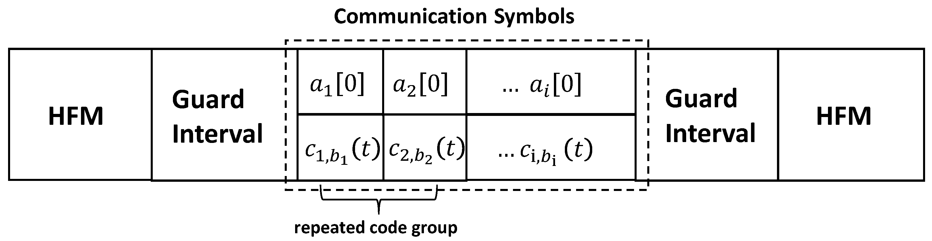
Number of the SS codes	50

, with the length of the original bit stream being 750 bits. The original bit stream is input into the transmitter structure illustrated in Figure 1, resulting in a total of 150 spread spectrum symbols carrying polar modulation, with the output data organized into frames of 50 symbols each, yielding a total of three frames. Regarding the carrier parameters, the center frequency is set to 6 kHz with a bandwidth of 4 kHz. The spreading code for the information sequence is a chaotic spreading code with a length of 511, operating at a rate of 4 kcps. During the simulation process, we incorporated three additional reception methods for comparison: 1. the conventional M-ary spread spectrum reception method without Doppler estimation (WDE-MSS); 2. the conventional M-ary spread spectrum reception method with coarse Doppler estimation (CDE-MSS); 3. the conventional M-ary spread spectrum reception method with fine Doppler estimation (FDE-MSS).

3.1. Constant Velocity Motion (CV)

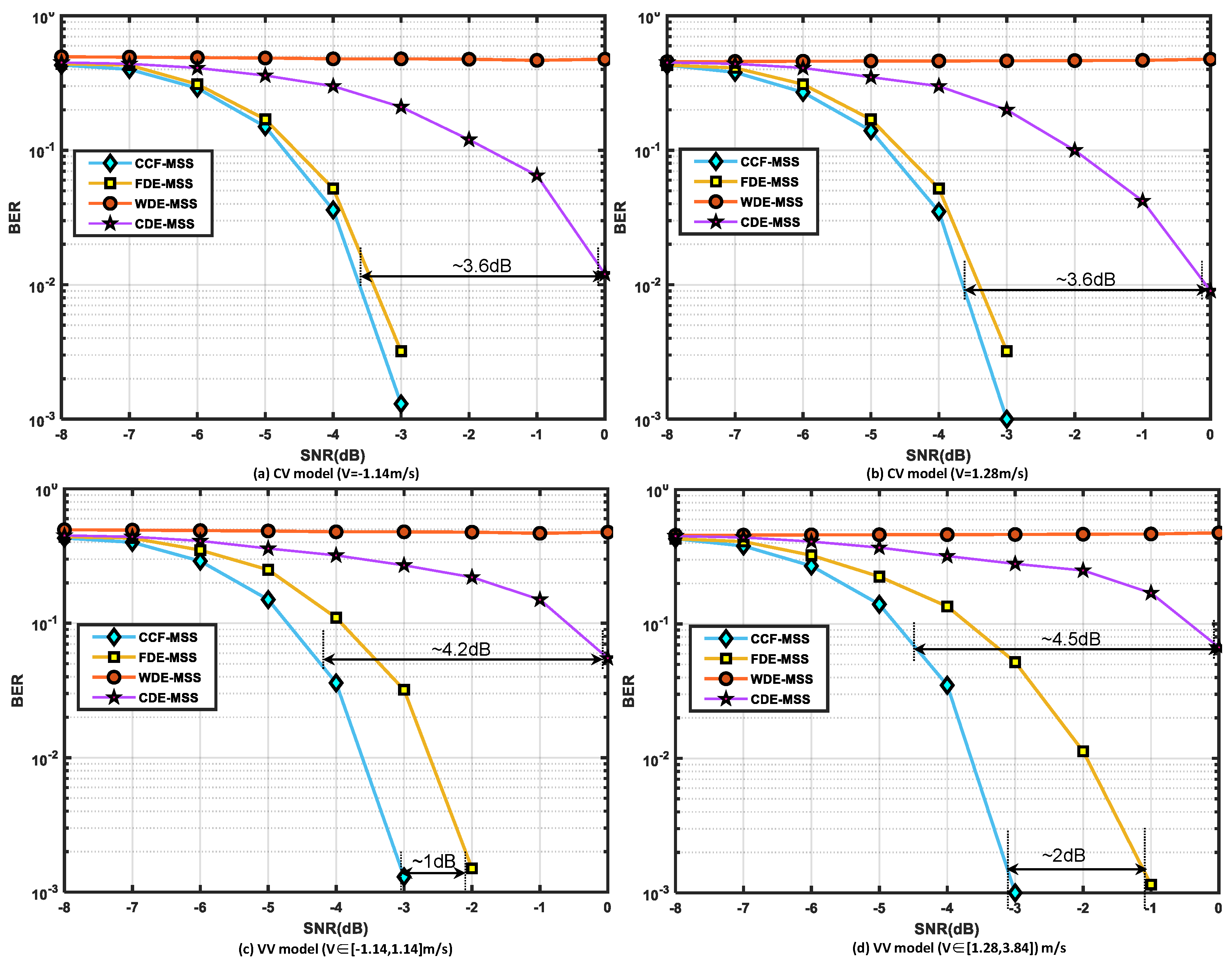
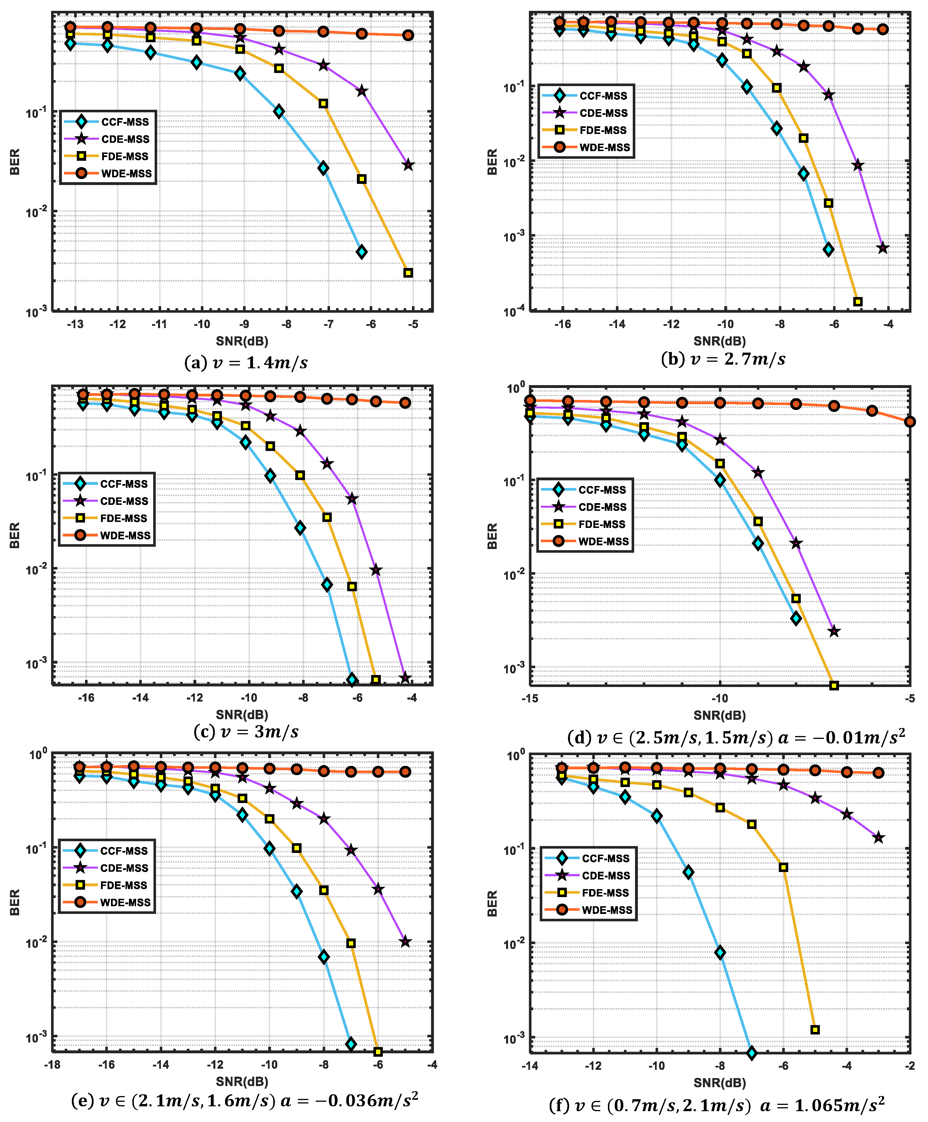
First, we evaluate the performance of CCF-MSS under constant velocity conditions. Given that the channel inherently exhibits time-varying Doppler (TVD) shifts, we directly add noise to the received signal to simulate the communication process under constant velocity conditions. Figure 5a,b illustrates the BER curves for different reception methods under constant velocity conditions.

It is evident that under the conditions of speeds of −1.14 m/s and 1.28 m/s, CCF-MSS exhibits the best performance, followed closely by FDE-MSS, though the decoding performance of the two methods shows only a slight difference. When the BER curve converges to ${10}^{-2}$ the performance loss of CDE-MSS compared to CCF-MSS is approximately 3.6 dB, while the performance of WDE-MSS, which does not employ Doppler estimation, is the poorest. Based on the simulation results, it is evident that CCF-MSS exhibits slightly better noise and Doppler resistance under constant velocity motion compared to FDE-MSS, and significantly outperforms CDE-MSS while demonstrating a clear superiority over WDE-MSS. This indicates that under conditions of large-scale relative motion, Doppler estimation and compensation are effective methods for mitigating the decline in spreading code correlation caused by frequency shifts.

3.2. Variable Velocity Motion (VV)

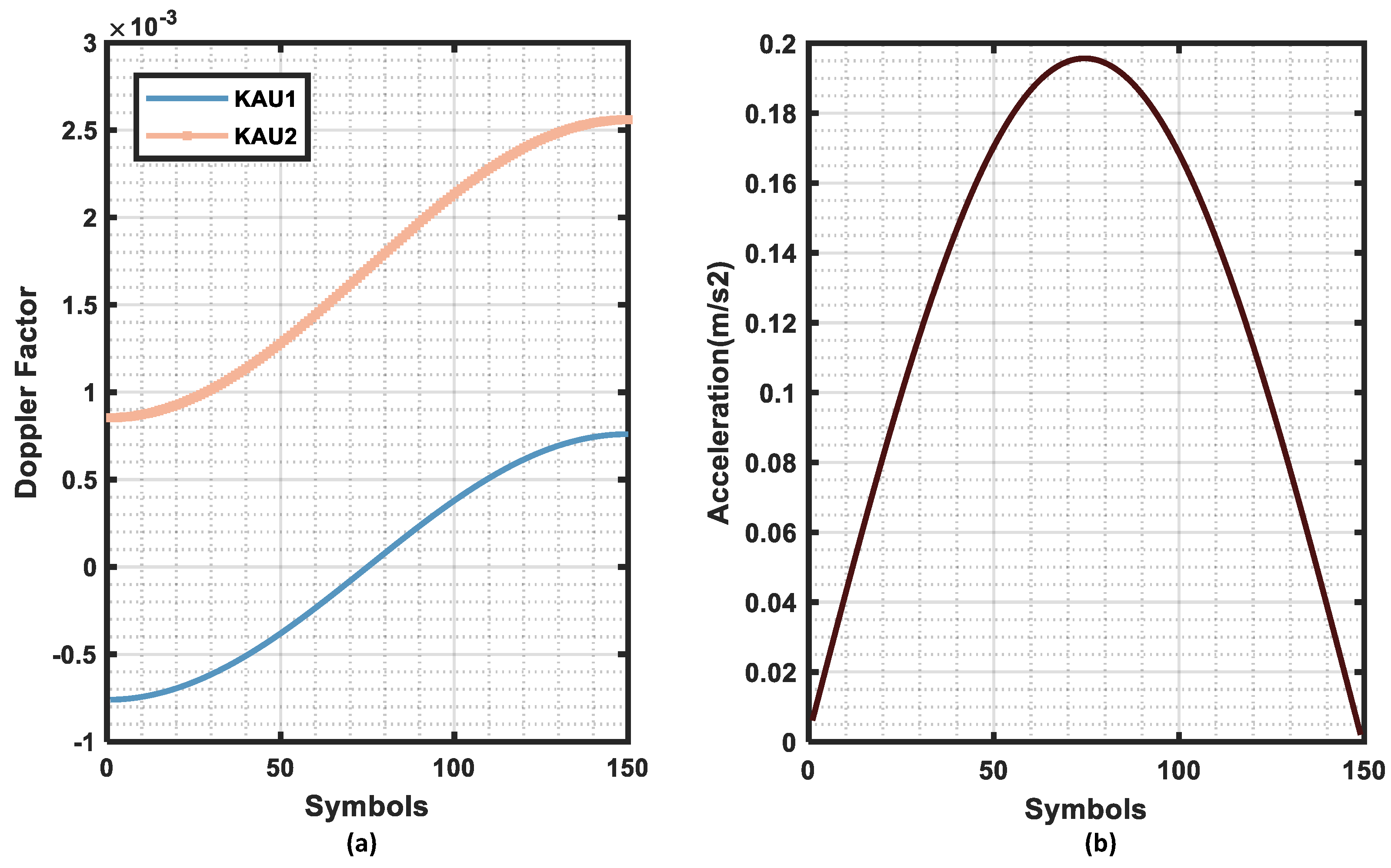
To better align with the communication process under actual underwater complex motion, we incorporated variable velocity motion conditions into the simulation, during which the Doppler factor varies within the duration of the signal, as shown in Figure 6a, while Figure 6b illustrates the variations in acceleration of the relative motion between the transmitter and receiver. The Doppler factor $\alpha \left(i\right)$ for the i-th symbol is given by the following:

$$\alpha \left(i\right)={\displaystyle \frac{v_0\pm v_0(1-cos\left(\frac{\pi i}{n}\right))}{c}},i=1,2,3...n$$

(22)

Here, n denotes the number of symbols in the transmitted signal, c represents the speed of sound, and $v_0$ denotes the initial velocity. Figure 5c,d presents the BER curves for variable speed motion under two simulated channels, and it is evident that CCF-MSS outperforms the other methods significantly. When the speed varies in the low-speed range $(-1.14$ m/s, 1.14 m/s), when the BER curve converges to ${10}^{-3}$, the performance loss of FDE-MSS compared to CCF-MSS is approximately 1 dB. When the speed varies in the high-speed range (1.28 m/s, 3.84 m/s) when the BER curve converges to ${10}^{-3}$, the performance loss of FDE-MSS compared to CCF-MSS is approximately 2 dB. The simulation results under variable speed motion conditions demonstrate that CCF-MSS exhibits superior resilience to speed variations compared to FDE-MSS, and when acceleration is constant while speed varies over a larger range, the performance gap becomes even more pronounced.

3.3. Doppler Tolerance

After analyzing the simulation results, it is evident that CCF-MSS significantly outperforms the other three traditional reception methods under time-varying channel conditions. Moreover, the coarse Doppler estimation steps for CCF-MSS, CDE-MSS, and FDE-MSS are entirely identical, while the subsequent decoding performance indicates that there are differences in tolerance to Doppler estimation errors among the three methods.

4. Validation Through Sea Trials

The simulation results indicate that the proposed reception method can effectively handle Doppler shifts caused by various motion patterns. However, the actual motion states of the targets are not as ideal as those in the numerical simulations. Therefore, we validated the true performance of the proposed reception method through sea trials.

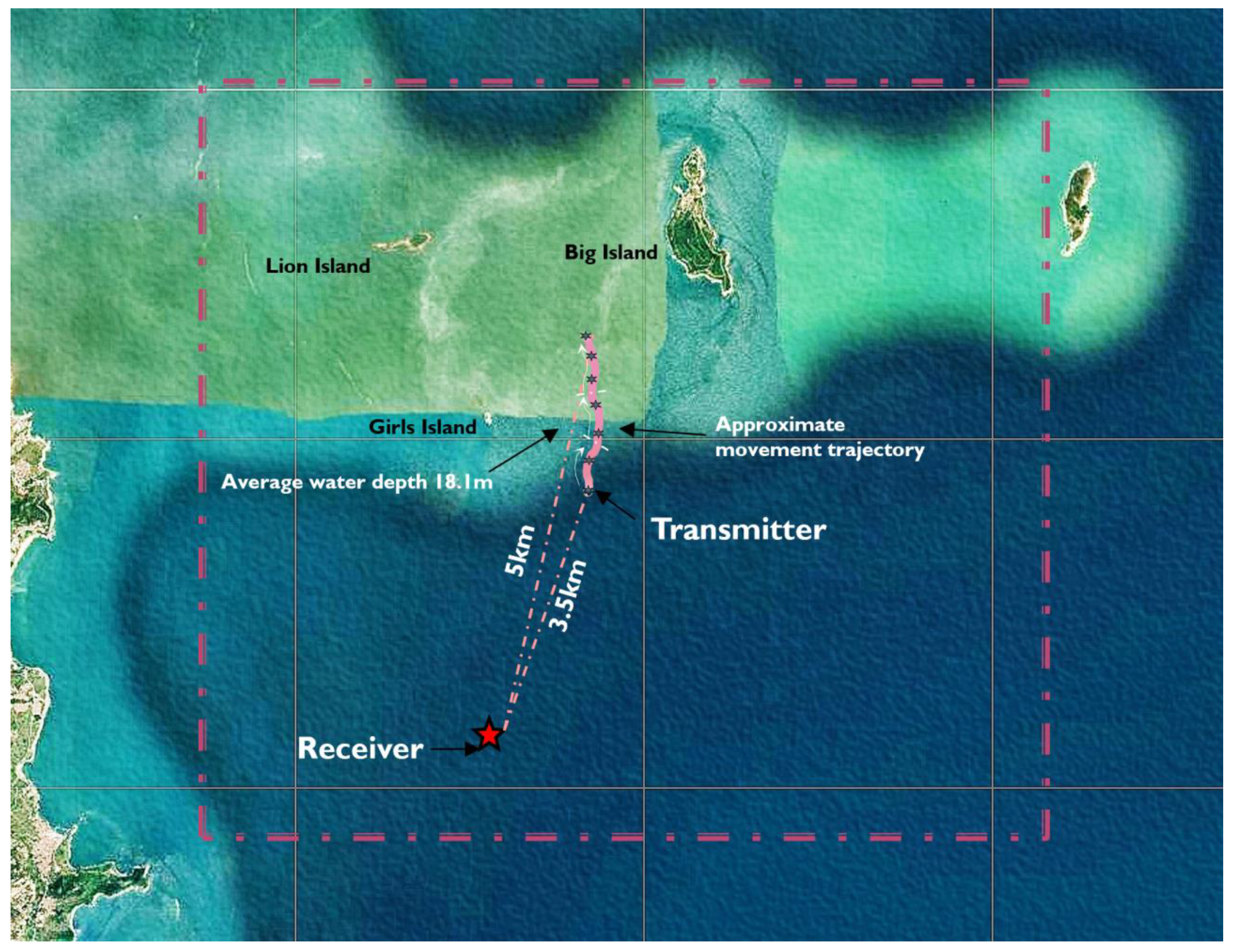
In March 2023, we conducted an underwater acoustic M-SS communication experiment in Laoshan Bay, China, with the experimental area location shown in Figure 7. During the experiment, the receiving vessel was anchored while the transmitting vessel was in motion, and the speed and direction of its movement were determined and recorded by the BeiDou satellite positioning system (BDS). The radial velocity was calculated based on the latitude and longitude measurements of both the transmitting and receiving vessels, and due to the measurement errors inherent in the BDS and the fact that the receiving vessel was not strictly fixed, there is a certain systematic error in the derived radial velocity. Both the transmitter and receiver were deployed at a depth of 10 m underwater, with the transmitter’s depth being inversely proportional to the speed of the transmitting vessel; the actual receiving depth was influenced by the relative motion of background currents and their own platforms, resulting in certain time variability.

The average water depth in the sea trial area is 18.1 m, with a gentle slope between the signal receiver and the transmitting vessel (excluding nearby islands and surrounding waters), and the water depth varies little, characterized by a muddy seabed. On the day of the trial, the weather was clear, with temperatures ranging from 8 to 15 °C, a south wind of 3 to 4 on the Beaufort scale, and wave heights of less than 0.5 m.

The entire sea trial process is divided into three groups. The distance between the receiver and transmitter ranges up to 3.5 km, with a maximum distance of 5 km. There is a significant variation in SNR among the different groups, with a maximum difference of up to 3 dB. The parameters of the transmitter are presented in Table 1. Similar to the aforementioned simulation process, we continue to use reception methods such as WDE-MSS, CDE-MSS, and FDE-MSS for comparison.

Table 2. The average SNR of different groups of sea test data and the BER processed by proposed receptions.

Test Groups	Average SNR (dB)	Different Receptions BER
		CCF-MSS	WDE-MSS	FDE-MSS	CDE-MSS
Group 1 (Section 4.1)	−3.4	0	0.7717	0.0055	0.0207
Group 2 (Section 4.2)	−4.7	0	0.7763	0.0027	0.0167
Group 3 (Section 4.3)	−6.5	0.0013	0.7745	0.0103	0.0324

presents the decoding results of the experimental data for each group. The average SNR of each frame signal is estimated using Equation (23), as follows:

$$SNR=10{log}_{10}\left({\displaystyle \frac{P_r-P_u}{P_u}}\right)$$

(23)

Here, $P_r$ represents the average power of the received signal during the duration of the communication signal, and $P_u$ denotes the average power of the noise signal during the communication gaps. To highlight the performance differences among the various reception methods, we first conduct a brief analysis of the sea trial data from each group and then select the portions of the sea trial data from each group that exhibit significant distortion for detailed analysis.

4.1. Processing and Analysis of the First Group of Sea Trial Data

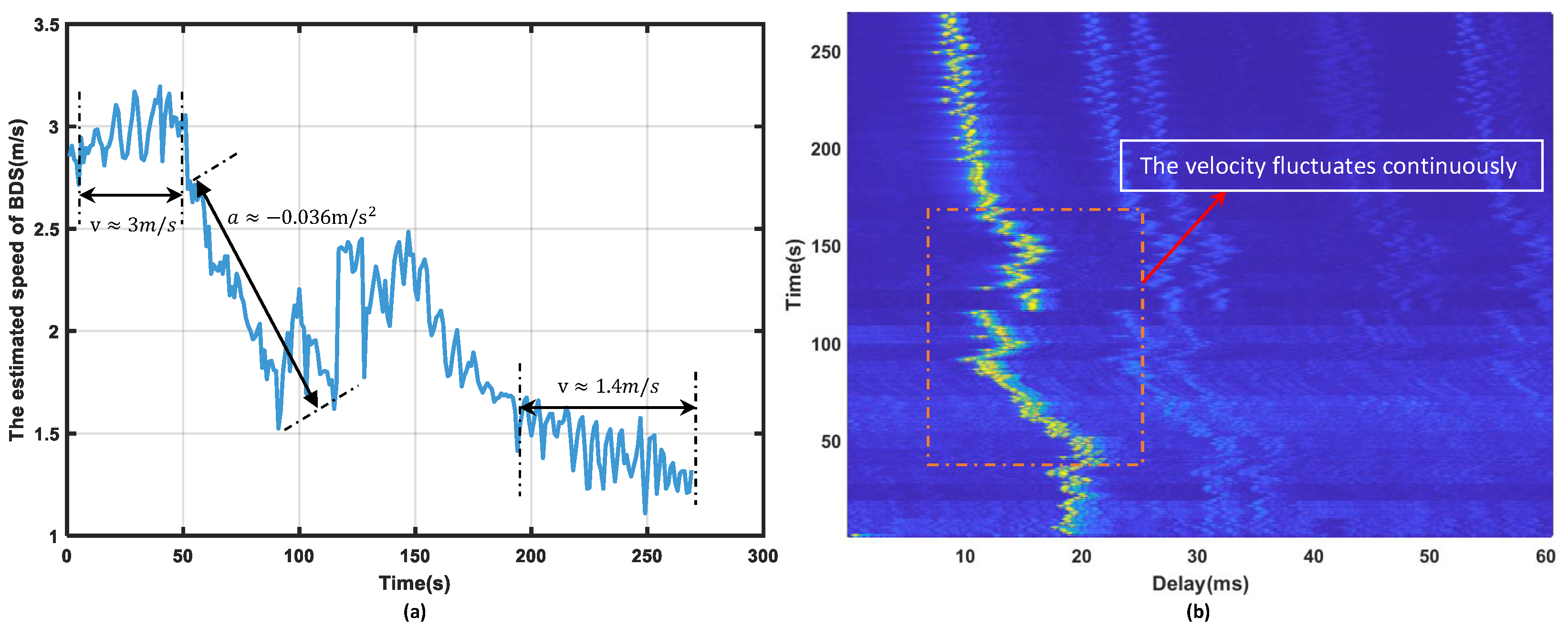
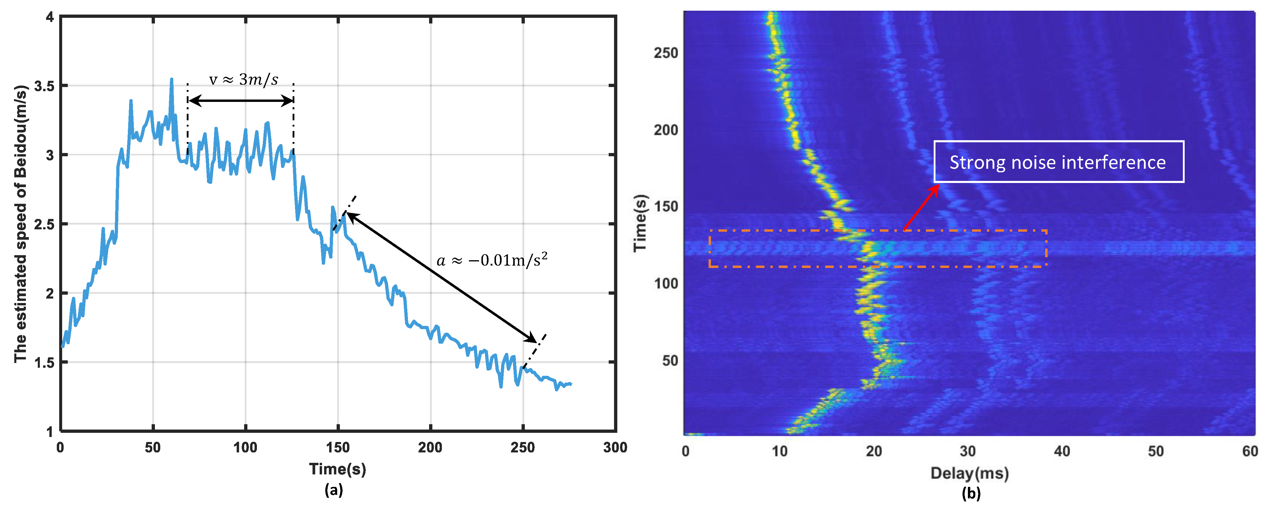
Figure 8a displays the speed recorded during the first sea trial process by the BDS, while Figure 8b presents the results of the channel impulse response. It is evident that the channel exhibits significant multipath effects during the communication process, with complex background noise and frequent instantaneous noise occurrences.

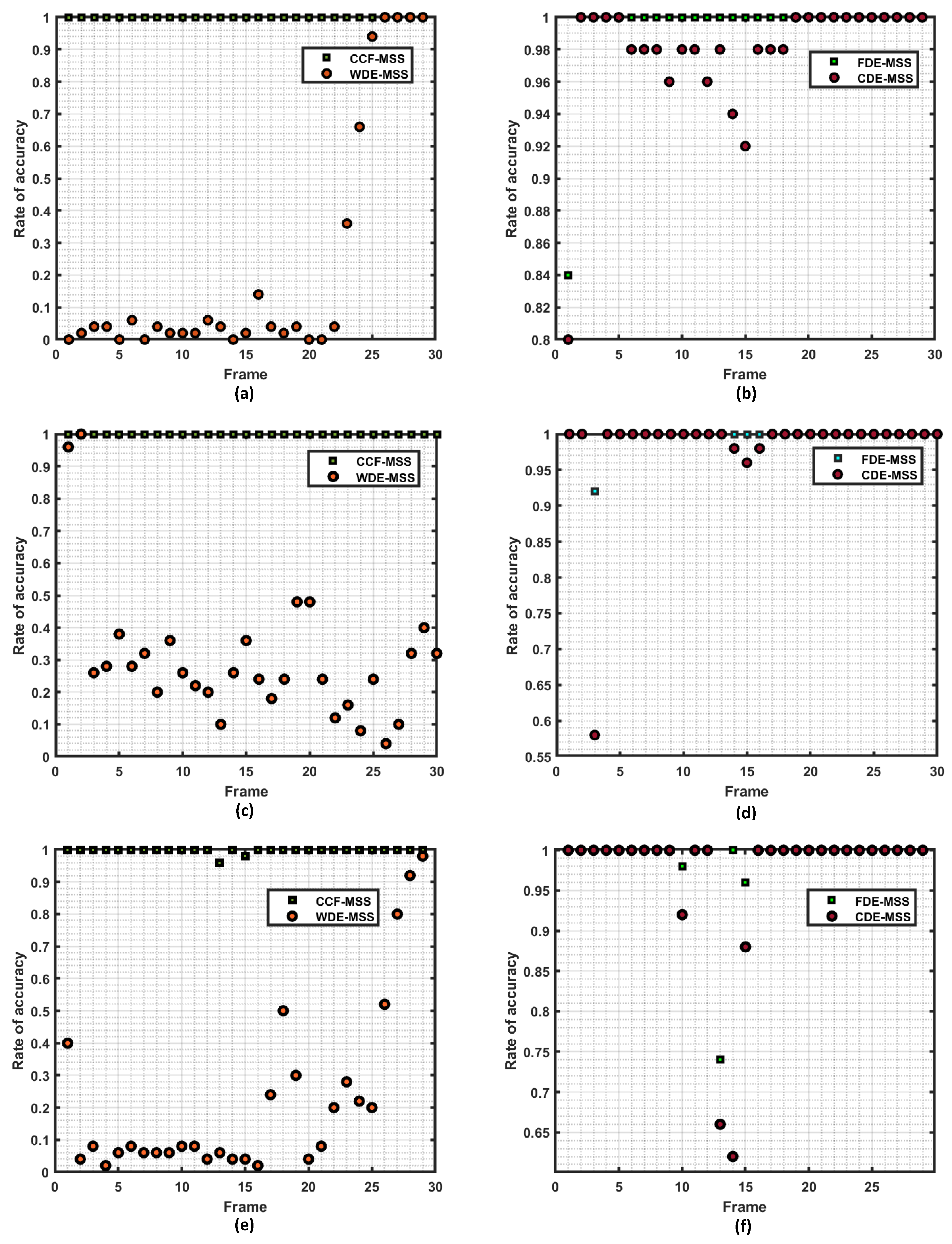
The frame accuracy in the first group of sea trials is depicted in Figure 9a,b, where CCF-MSS exhibits a BER of 0, indicating superior decoding performance. WDE-MSS achieved zero bit errors only in frames 26 to 29, while achieving an accuracy of 0.9 in frame 25, resulting in an overall error rate of 0.7717. The reason for this can be attributed to the decrease in vessel speed during the later stages of the trial, which significantly reduced the Doppler effect, thus restoring decoding capability. When using CDE-MSS, several frames in the middle experienced bit errors, which was due to inaccurate coarse Doppler estimation during the variable speed process, resulting in incorrect compensation of the CFO value, with an overall error rate of 0.0275. The decoding performance of FDE-MSS is significantly better than that of the other two traditional methods, indicating that fine Doppler estimation is an effective means to overcome the Doppler shifts caused by complex time-varying channels, with a total BER of 0.0055. Except for the significant difference in the processing results of the first frame, the decoding performances of FDE-MSS and CCF-MSS were comparable during this group of sea trials. The following section will analyze the decoding results of the first frame for both FDE-MSS and CCF-MSS. The time duration of the first frame signal in the figure is approximately 0 to 10 s. It can be observed that the vessel speed is relatively high, reaching up to 3 m/s, with complex background noise and pronounced multipath effects. 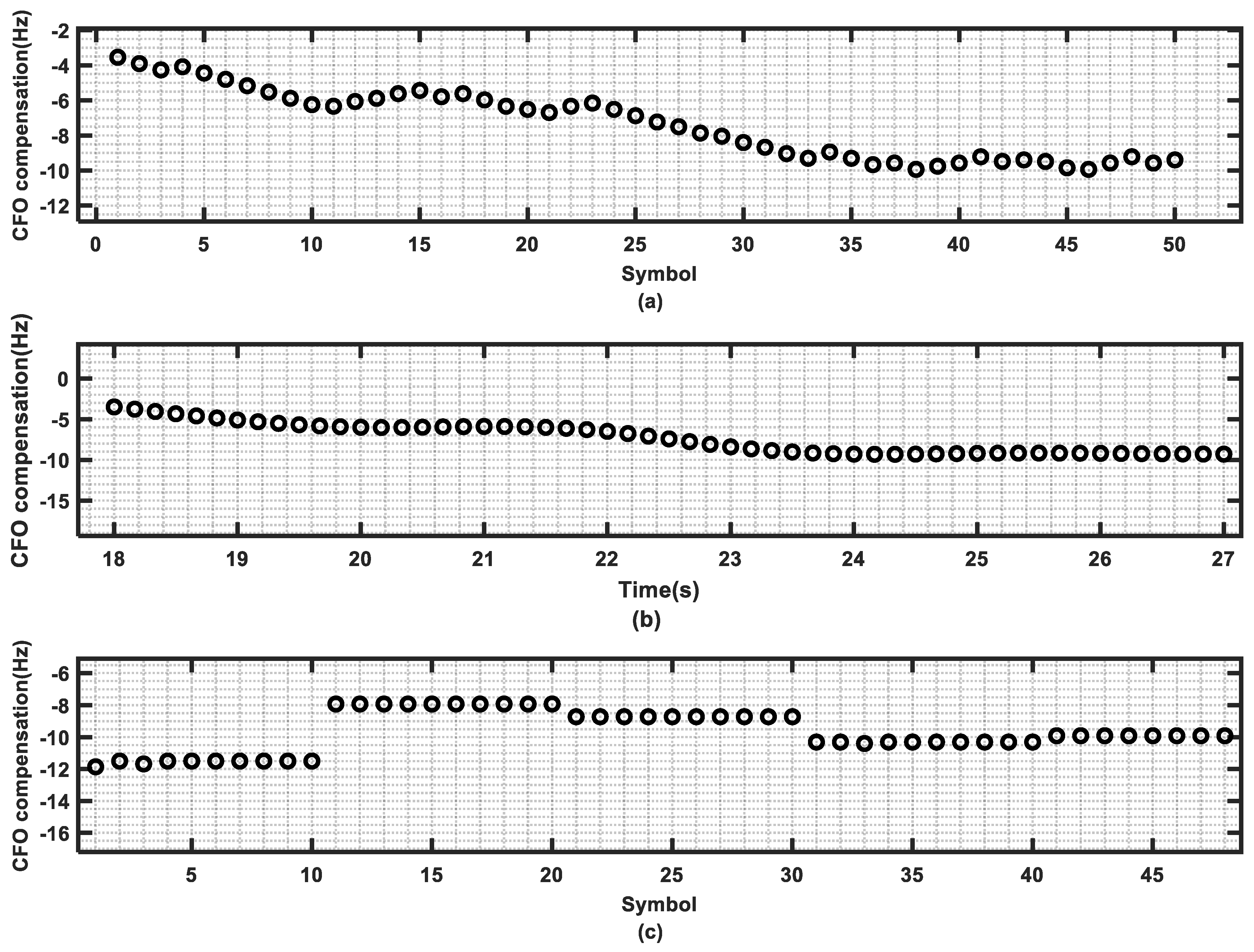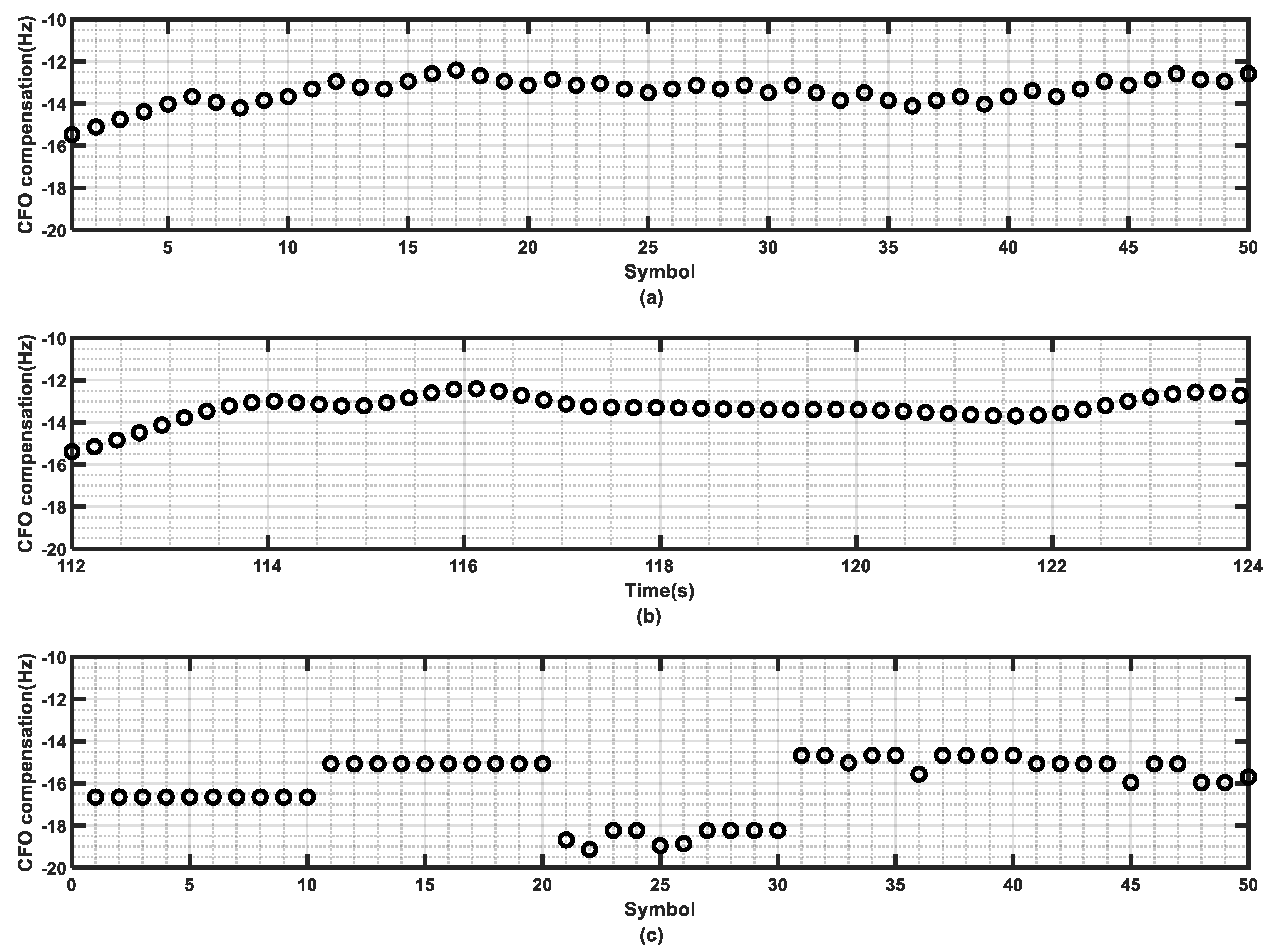Figure 10a,c shows the final output of the CFO compensation values for CCF-MSS and FDE-MSS in the first frame, while Figure 10b presents the CFO values calculated from the vessel speed output by the BDS, which can be used as a reference for the actual CFO for comparison. It can be observed that the CFO estimated by CCF-MSS is largely consistent with the CFO calculated from the BeiDou output speed, indicating that the decoding performance is quite good. However, the CFO compensated by FDE-MSS differs significantly from the measured CFO during symbols 30 to 40. Upon inspection, decoding errors were found in FDE-MSS for symbols 31 to 37. The following section will analyze the despreading results for the specific symbols.

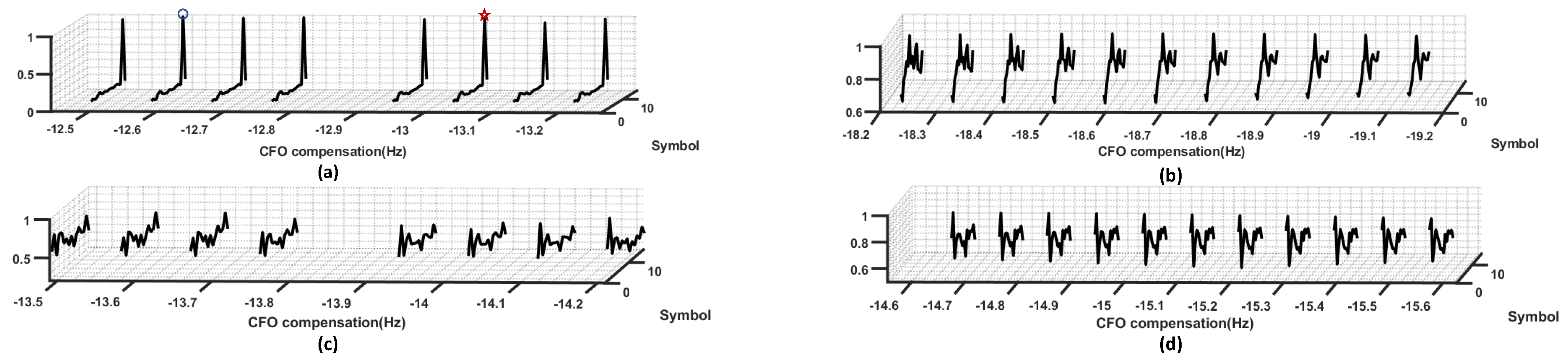
We compared the despreading correlation peaks of the 32nd and 33rd symbols under both CCF-MSS and FDE-MSS reception methods. Figure 11a presents the despreading result for symbol 32 under CCF-MSS, where the blue circles indicate the maximum peaks under different CFO compensations, and the red pentagons represent the peaks under CFO compensation selected based on the correlation cost factor. We can observe that the position of the output maximum peak corresponds to a CFO compensation of −14.7 Hz, while the correct CFO compensation position for the next symbol is −13.8 Hz (see Figure 11c). This indicates that relying on the maximum correlation peak to select the CFO compensation position can lead to inaccuracies, whereas using the correlation cost factor allows for the selection of CFO compensation values that align with the correct frequency shift trend. Figure 11b,d shows the despreading results for symbols 32 and 33 under different CFO compensations for FDE-MSS, which are completely erroneous. From Figure 11, it is evident that there are significant differences in the range of CFO compensations between the two reception methods, which can be attributed to the fact that FDE-MSS did not utilize the cost factor for Doppler estimation, resulting in inaccuracies in the estimation direction, leading to a gradual accumulation of errors and subsequent decoding issues.

4.2. Processing and Analysis of the Second Group of Sea Trial Data

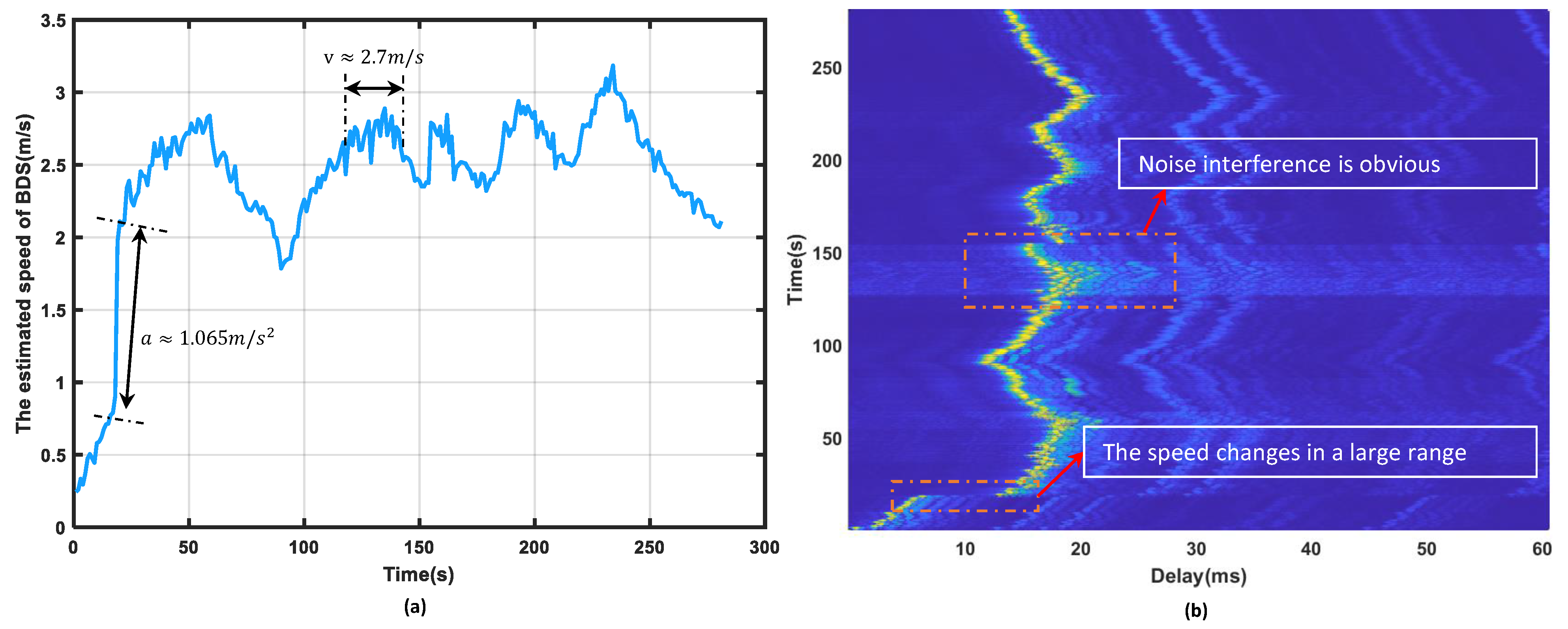
Figure 12a displays the speed recorded during the second sea trial process by the BDS, while Figure 12b presents the results of the channel impulse response. It is evident that the channel exhibits significant multipath effects during the communication process, and the background noise interference is quite strong.

Figure 9b,d presents the frame accuracy for the second group of trial processes. CCF-MSS maintains a zero bit error rate in each frame, whereas WDE-MSS demonstrates good decoding performance in the first two frames, corresponding to a time period of approximately 1 to 18 s. Based on the radial velocity data output from the BDS, the system is currently in an acceleration phase, with corresponding speeds ranging from approximately 0.3 to 0.7 m/s, and the corresponding acceleration is approximately 0.036 m/s². The performance of WDE-MSS deteriorates significantly after the third frame, and both CDE-MSS and FDE-MSS also exhibit bit errors. As seen in Figure 12a, there is a significant change in speed at the beginning of the third frame, with the maximum acceleration during the entire third frame reaching 1.065 m/s². The following section will analyze the decoding process of the third frame data from the second group of trials.

Following the same analytical approach as previously discussed, we first analyze the CFO compensation results for the third frame data, as shown in Figure 13. At the beginning of the third frame, there is a significant change in CFO due to the high acceleration at that moment, and the CFO compensation results of CCF-MSS are largely consistent with the results calculated from the radial velocity output by the BDS, showing a similar trend of variation. However, the CFO values compensated by WDE-MSS exhibit significant discrepancies. Taking the despreading results of the third and fourth symbols in the third frame as an example, Figure 14 displays the correlation peaks for symbols 3 and 4 in the third frame, CCF-MSS shows a favorable despreading performance for symbols 1 and 2, with very sharp peaks, minimal interference, and correct decoding. During the despreading process of the second symbol, only two CFO searches were conducted, which was due to the accurate estimation of the CFO that met the preset threshold for the correlation cost factor ahead of time, leading to the termination of the search. This also reflects the efficiency of the CCF-MSS system. Figure 14b,d shows the despreading results for FDE-MSS, both of which are erroneous. According to the results of the second group of experiments, compared to FDE-MSS, CCF-MSS exhibits stronger resilience to acceleration and higher Doppler tolerance, allowing for correct decoding at an acceleration of 1.065 m/s².

4.3. Processing and Analysis of the Third Group of Sea Trial Data

Through the analysis of the aforementioned sea trial data, it can be concluded that CCF-MSS outperforms other reception methods under conditions of high speed and high acceleration. Next, we analyzed the noise resistance performance of CCF-MSS based on the third group of data. Figure 15 illustrates the speed and channel impulse response during the third group of sea trials. It is evident that significant noise interference occurred during the third group of sea trials. Figure 9e,f displays the frame accuracy for decoding using different methods. It can be observed that during periods of strong noise interference, the performance of WDE-MSS and CDE-MSS significantly deteriorates, whereas CCF-MSS maintains a high accuracy rate, indicating that the use of the CCF-MSS reception method can still achieve high spreading gain under high-speed conditions, demonstrating a stronger noise resilience capability.

In the processing of the third group of data, the BER for FDE-MSS and CDE-MSS is relatively high at frame 13, which corresponds to the position of the white box in Figure 15, indicating that there is significant noise interference at this time. Figure 16 presents the CFO compensation results for frame 13. It can be observed that the CFO compensation results of CCF-MSS are largely consistent with the speed compensation results output by the BDS, while significant discrepancies are noted for FDE-MSS at symbols 20 and 31. We analyze that this is due to the high noise levels at that time, where the decline in spreading gain caused by frequency offset cannot overcome the prevailing noise environment. The following section will illustrate the despreading correlation peaks for symbols 21 and 31 in frame 13 as examples. Symbol 21 is correctly decoded using the CCF-MSS reception method, and while it is incorrectly decoded by the FDE-MSS reception method, Symbol 31 is incorrectly decoded by both methods. Figure 17 illustrates the despreading correlation peaks for symbols 21 and 31 in frame 13. It can be observed that the range of CFO compensations for symbol 21 differs significantly between the two reception methods. This also indicates that even under high noise conditions, the accuracy of Doppler estimation using correlation cost factors remains high. During the CFO compensation process for symbol 31, although the CFO compensation results from both methods are quite similar to the output results of the BDS, neither method is able to achieve correct decoding. We attribute this decoding failure to the high instantaneous noise levels.

4.4. Processing and Analysis of Sea Trial Data with Added Ocean Noise

After processing and analyzing the data from the three groups of trials, we can conclude that, under conditions where noise interference is not significant, the decoding performance of the four reception methods is relatively similar during low-speed operation. During high-speed operation, the decoding performance of WDE-MSS deteriorates significantly, while the performance of the other three reception methods remains relatively comparable. In situations with significant acceleration variations, only CCF-MSS is able to maintain good decoding performance, while the performance of the other three reception methods declines substantially. When there is significant noise interference and high-speed operation, only CCF-MSS can maintain good decoding performance. In summary, CCF-MSS exhibits superior resilience to speed variations, acceleration, and noise interference. The following section will process different portions of the three groups of sea trial data, incorporating measured ocean noise, to supplement the aforementioned analysis results.

4.4.1. Extraction of Ocean Noise

On the day of the experiment, multiple sets of sea trial noise were extracted at different time intervals, and the different groups of noise were mixed in random proportions before being added to various portions of the sea trial data for Monte Carlo simulations.

4.4.2. Extraction of Data Under Different Motion States from Sea Trials

Due to significant variations in motion states within each data group and substantial differences between the motion states of different groups, to more clearly demonstrate the superiority of the CCF-MSS reception method, we extracted sea trial data based on different motion states.The data were extracted based on six motion states: $V=1.4$ m/s, $V=2.7$ m/s, $V=3$ m/s, $a=-0.01$ m/s², $a=-0.036$ m/s², and $a=1.065$ m/s², and ocean trial noise was added to these states. The BER curves are shown in Figure 18.

Based on the processing of the sea trial data, we can draw the following conclusions: 1. Under low signal-to-noise ratio and complex motion conditions, CCF-MSS demonstrates superior noise resistance, speed resilience, and acceleration tolerance compared to other reception methods. At a speed of 3 m/s, when the bit error rate reaches ${10}^{-3}$, the performance of CCF-MSS improves by approximately 1 dB and 2 dB compared to FDE-MSS and CDE-MSS, respectively. Furthermore, when the acceleration is 1.065 m/s², at the same BER level, the performance improves by approximately 4 dB compared to FDE-MSS. As the noise intensity increases to a certain level, the performance gap gradually widens. However, when the noise becomes excessively high, the performance differences begin to diminish. 2. Doppler shifts generated by motion can be compensated for through Doppler estimation; however, when acceleration is substantial, the errors generated by coarse Doppler estimation can also be significant, making it easy for the FDE-MSS reception method to yield inaccurate estimates of the frequency shift direction, which results in cumulative errors. In such cases, it is essential to utilize correlation cost factors for subsequent estimations, accurately confining the range of Doppler frequency shift variations within the search interval. 3. Inaccurate Doppler estimation can lead to a significant reduction in spreading gain, resulting in diminished noise resistance, which indicates that the noise resistance of CCF-MSS is attributed to its precise Doppler estimation capability.

5. Conclusions

This paper addresses the challenges of low signal-to-noise ratio and significant time-varying Doppler effects in mobile underwater acoustic communication by proposing a CCF-MSS reception scheme. By utilizing correlation cost factors to assess the accuracy of Doppler estimation, the method performs symbol-by-symbol Doppler estimation to achieve dynamic CFO compensation and addresses the issue of energy reduction caused by signals with significant CFO deviations passing through band-limited filters. The proposed method does not require complex speed estimation and significantly enhances Doppler tolerance. Simulation analyses and sea trial data confirm that CCF-MSS exhibits superior resistance to Doppler frequency shifts and noise compared to the FDE-MSS, CDE-MSS, and WDE-MSS reception methods used for comparison across various motion modes. Additionally, it demonstrates high computational efficiency, making it suitable for real-time underwater acoustic communication. In future work, we plan to conduct additional experiments in mobile underwater acoustic communication, to validate the robustness of the proposed system, and to extend single-to-single system communication to single-to-multiple system communication.

References

1. Haibin, W.; Lixin, W. Long-range underwater acoustic communication based on chaotic-fm m-ary mode. Acta Acust. 2004, 29, 161–166. [Google Scholar]
2. Xu, X.; Zhou, S.; Morozov, A.K.; Preisig, J.C. Per-survivor processing for underwater acoustic communications with direct-sequence spread spectrum. J. Acoust. Soc. Am. 2013, 133, 2746–2754. [Google Scholar] [CrossRef] [PubMed]
3. Song, H.; Hodgkiss, W.S.; Walree, P.V. Phase-coherent communications without explicit phase tracking. J. Acoust. Soc. Am. 2010, 128, 969–972. [Google Scholar] [CrossRef]
4. Qu, F.; Yang, L.; Yang, T. High reliability direct-sequence spread spectrum for underwater acoustic communications. In Proceedings of the OCEANS 2009, Biloxi, MS, USA, 26–29 October 2009; pp. 1–6. [Google Scholar]
5. Yoo, K.B.; Edelmann, G.F. Low complexity multipath and doppler compensation for direct-sequence spread spectrum signals in underwater acoustic communication. Appl. Acoust. 2021, 180, 108094. [Google Scholar] [CrossRef]
6. Dillard, R.A. Detectability of spread-spectrum signals. IEEE Trans. Aerosp. Electron. Syst. 1979, AES-15, 526–537. [Google Scholar] [CrossRef]
7. Loubet, G.; Capellano, V.; Filipiak, R. Underwater spread-spectrum communications. In Proceedings of the Oceans ’97. MTS/IEEE Conference Proceedings, Halifax, NS, Canada, 6–9 October 1997; Volume 1, pp. 574–579. [Google Scholar]
8. Freitag, L.; Stojanovic, M.; Singh, S.; Johnson, M. Analysis of channel effects on direct-sequence and frequency-hopped spread-spectrum acoustic communication. IEEE J. Ocean. Eng. 2001, 26, 586–593. [Google Scholar] [CrossRef]
9. Kaddoum, G.; Ahmed, M.F.; Nijsure, Y. Code index modulation: A high data rate and energy efficient communication system. IEEE Commun. Lett. 2014, 19, 175–178. [Google Scholar] [CrossRef]
10. Kaddoum, G.; Nijsure, Y.; Tran, H. Generalized code index modulation technique for high-data-rate communication systems. IEEE Trans. Veh. Technol. 2015, 65, 7000–7009. [Google Scholar] [CrossRef]
11. Cui, H.; Liu, C.; Si, B.; Wu, J.; Sun, D. Iterative receiver for the triple differential psk modulation in the time-varying underwater acoustic communications. IET Commun. 2020, 14, 2813–2819. [Google Scholar] [CrossRef]
12. Yaohui, H.; Shuping, H.; Jianbo, L.; Qi, Z.; Yanhou, Z. Combination differential direct sequence spread spectrum algorithm for mobile underwater acoustic communication. J. Electron. Inf. Technol. 2022, 44, 6. [Google Scholar]
13. Hu, Y.; Han, S.; Li, H.; Zhao, H.; Yang, G.; Xu, J. Tcn-based m-ary mobile spread spectrum underwater acoustic communication. Appl. Acoust. 2023, 211, 109457. [Google Scholar] [CrossRef]
14. Sun, D.; Hong, X.; Cui, H.; Liu, L. A symbol-based passband doppler tracking and compensation algorithm for underwater acoustic dsss communications. J. Commun. Inf. Netw. 2020, 5, 168–176. [Google Scholar] [CrossRef]
15. Abdelkareem, A.E.; Sharif, B.S.; Tsimenidis, C.C. Adaptive time varying doppler shift compensation algorithm for ofdm-based underwater acoustic communication systems. Ad Hoc Netw. 2016, 45, 104–119. [Google Scholar] [CrossRef]
16. Sharif, B.S.; Neasham, J.; Hinton, O.R.; Adams, A.E. A computationally efficient doppler compensation system for underwater acoustic communications. IEEE J. Ocean. Eng. 2000, 25, 52–61. [Google Scholar] [CrossRef]
17. Freitag, L.; Stojanovic, M. Mmse acquisition of dsss acoustic communications signals. In Oceans’ 04 MTS/IEEE Techno-Ocean’04 (IEEE Cat. No. 04CH37600); IEEE: New York, NY, USA, 2004; Volume 1, pp. 14–19. [Google Scholar]
18. Neasham, J.; Corner, T.; Davies, J.; Hamilton, A. Sea trial results and receiver performance analysis for phorcys v0 waveform. In Proceedings of the 2022 Sixth Underwater Communications and Networking Conference (UComms), Lerici, Italy, 30 August–1 September 2022; IEEE: New York, NY, USA, 2022; pp. 1–5. [Google Scholar]
19. Sun, D.; Wu, J.; Hong, X.; Liu, C.; Cui, H.; Si, B. Iterative double-differential direct-sequence spread spectrum reception in underwater acoustic channel with time-varying doppler shifts. J. Acoust. Soc. Am. 2023, 153, 1027–1041. [Google Scholar] [CrossRef] [PubMed]
20. Qu, F.; Wang, Z.; Yang, L.; Wu, Z. A journey toward modeling and resolving doppler in underwater acoustic communications. IEEE Commun. Mag. 2016, 54, 49–55. [Google Scholar] [CrossRef]
21. Van Walree, P.A. Propagation and scattering effects in underwater acoustic communication channels. IEEE J. Ocean. Eng. 2013, 38, 614–631. [Google Scholar] [CrossRef]
22. Yang, T. Temporal resolutions of time-reversal and passive-phase conjugation for underwater acoustic communications. IEEE J. Ocean. Eng. 2003, 28, 229–245. [Google Scholar] [CrossRef]
23. Yang, T. Correlation-based decision-feedback equalizer for underwater acoustic communications. IEEE J. Ocean. Eng. 2005, 30, 865–880. [Google Scholar] [CrossRef]
24. Zakharov, Y.V.; Morozov, A.K. Ofdm transmission without guard interval in fast-varying underwater acoustic channels. IEEE J. Ocean. Eng. 2014, 40, 144–158. [Google Scholar] [CrossRef]
25. Pengyu, D.; Longxiang, G.; Jingwei, Y.; Gang, Q. Mobile direct-sequence spread-spectrum underwater acoustic communication based on improved differential energy detector. J. Commun. 2017, 38, 144–153. [Google Scholar]
26. Liu, Z.; Yoo, K.; Yang, T.; Cho, S.E.; Song, H.; Ensberg, D.E. Long-range double-differentially coded spread-spectrum acoustic communications with a towed array. IEEE J. Ocean. Eng. 2013, 39, 482–490. [Google Scholar] [CrossRef]
27. Xiaoming, L.; He, Z.; Haowei, W.; Jinglan, O. Rapid dsss signal acquisition algorithm under high dynamic environment. J. Electron. Inf. Technol. 2016, 38, 1398–1405. [Google Scholar]
28. Yang, T. Properties of underwater acoustic communication channels in shallow water. J. Acoust. Soc. Am. 2012, 131, 129–145. [Google Scholar] [CrossRef] [PubMed]
29. Li, B.; Zhou, S.; Stojanovic, M.; Freitag, L.; Willett, P. Multicarrier communication over underwater acoustic channels with nonuniform doppler shifts. IEEE J. Ocean. Eng. 2008, 33, 198–209. [Google Scholar]
30. Yang, G.; Zhou, F.; Lou, Y.; Qiao, G.; Ahmed, N.; He, Y. Double-differential coded m-ary direct sequence spread spectrum for mobile underwater acoustic communication system. Appl. Acoust. 2021, 183, 108303. [Google Scholar] [CrossRef]
31. van Walree, P.A.; Socheleau, F.-X.; Otnes, R.; Jenserud, T. The watermark benchmark for underwater acoustic modulation schemes. IEEE J. Ocean. Eng. 2017, 42, 1007–1018. [Google Scholar] [CrossRef]
Figure 1. Underwater acoustic communication system model.
Jmse 12 02151 g001
Figure 2. Doppler estimation process.
Jmse 12 02151 g002
Figure 3. Frame structure.
Jmse 12 02151 g003
Figure 4. Time-varying channel impulse response (TVCIR) of KAU1 and KAU2, including both a 3D representation of the channel and its 2D projections.
Jmse 12 02151 g004
Figure 5. The BER curves for different reception methods under two types of channels with varying motion states are presented: (a) represents the BER curve for constant velocity motion under the KAU1 channel; (b) represents the BER curve for constant velocity motion under the KAU2 channel; (c) represents the BER curve for variable velocity motion under the KAU1 channel; (d) represents the BER curve for variable velocity motion under the KAU2 channel.
Jmse 12 02151 g005
Figure 6. (a) illustrates the variation in Doppler factors during variable velocity motion under two types of channels; (b) depicts the changes in acceleration during variable velocity motion under both channels (with identical acceleration variations).
Jmse 12 02151 g006
Figure 7. Map of sea trial scope of Laoshan Bay.
Jmse 12 02151 g007
Figure 8. (a) is the speed of the first group processes recorded by BDS. (b) is the first group processes channel impulse response.
Jmse 12 02151 g008
Figure 9. The accuracy rates of each frame obtained by different methods: (a,b) correspond to the first sea trial, (c,d) correspond to the second sea trial, and (e,f) correspond to the third sea trial.
Jmse 12 02151 g009
Figure 10. (a) is the CFO compensation estimated by CCF-MSS, (b) is the CFO compensation estimated by BDS output speed, (c) is the CFO compensation estimated by FDE-MSS (first group).
Jmse 12 02151 g010
Figure 11. (a,c) is despreading correlation peaks of symbols 32 and 33 by CCF-MSS, (b,d) is despreading correlation peaks of symbols 32 and 33 by FDE-MSS (first frame of first group).
Jmse 12 02151 g011
Figure 12. (a) is the speed of the second group processes recorded by BDS, (b) is the second group processes channel impulse response.
Jmse 12 02151 g012
Figure 13. (a) is the CFO compensation estimated by CCF-MSS, (b) is the CFO compensation estimated by BDS output speed, (c) is the CFO compensation estimated by FDE-MSS (second group).
Jmse 12 02151 g013
Figure 14. (a,c) is despreading correlation peaks of symbols 3 and 4 by CCF-MSS, (b,d) is despreading correlation peaks of symbols 3 and 4 by FDE-MSS (third frame of second group).
Jmse 12 02151 g014
Figure 15. (a) is the speed of the third group processes recorded by BDS, (b) is the third group processes channel impulse response.
Jmse 12 02151 g015
Figure 16. (a) is the CFO compensation estimated by CCF-MSS, (b) is the CFO compensation estimated by BDS output speed, (c) is the CFO compensation estimated by FDE-MSS (third group).
Jmse 12 02151 g016
Figure 17. (a,c) is despreading correlation peaks of symbols 21 and 31 by CCF-MSS, (b,d) is despreading correlation peaks of symbols 21 and 31 by FDE-MSS (thirteen frame of third group).
Jmse 12 02151 g017
Figure 18. BER curves of sea trial data with random ocean noise added under different motion states.
Jmse 12 02151 g018