Data-Driven Based Path Planning of Underwater Vehicles Under Local Flow Field

Abstract

Navigating through complex flow fields, underwater vehicles often face insufficient thrust to traverse particularly strong current areas, necessitating consideration of the physical feasibility of paths during route planning. By constructing a flow field database through Computational Fluid Dynamics (CFD) simulations of the operational environment, we were able to analyze local uncertainties within the flow field. Our investigation into path planning using these flow field data has led to the proposal of a hierarchical planning strategy that integrates global sampling with local optimization, ensuring both completeness and optimality of the planner. Initially, we developed an improved global sampling algorithm derived from RRT to attain nearly optimal theoretical feasible solutions on a global scale. Subsequently, we implemented corrective measures using directed expansion to address locally infeasible sections. The algorithm’s efficacy was theoretically validated, and simulated results based on real flow field environments were provided.

1. Introduction

Autonomous Underwater vehicles (AUVs) present a safer and more reliable alternative to manual operations for underwater detection and complex tasks, owing to their consistent performance and prolonged operational capabilities. Path planning stands as a pivotal factor in achieving autonomous control for AUVs and is essential for ensuring reliability and mission success [1]. For accomplishing specific tasks, vehicles need to demonstrate heightened environmental awareness and swiftly devise a practical trajectory [2]. The influence of water flow on the movement of underwater vehicles cannot be ignored. Properly handling the interaction between water flow and underwater vehicles will help find an optimal route that meets the requirements.

When the current in the environment is more complex, it will cause not only more energy consumption, but also feasibility issues in areas with strong current. This situation will cause some algorithms to offer invalid paths. Michael Soulignac et al. [3] argue that the reason for this phenomenon lies in the algorithm’s utilization of ineffective cost functions, resulting in some theoretically reachable grid cells being practically unreachable. By combining appropriate cost functions with continuous optimization techniques, they have proposed a Sliding Wavefront Expansion approach, addressing the effectiveness and global optimality issues in path planning within strong flow fields. This method can effectively avoid the influence of strong current areas, but the global traversal calculation will take a lot of time. On the other hand, Kruger et al. [4], leveraging a tidal river area flow model, selected suitable paths in both time and space, allowing the vehicle to navigate around counterflows that the propellers cannot overcome due to excessive current speeds, while also exploiting downstream flows to achieve significantly faster speeds than those attainable by the propellers, thereby achieving substantial energy savings.

Scholars have studied the path planning problem of underwater vehicles under the influence of currents from different perspectives. According to the predictability of flow field information, path planning methods can be roughly divided into two categories. When the flow field information is unpredictable, there are methods like Case-based reasoning [5], the wavefront expansion method, and reinforcement learning-based methods [6,7]. They can correct the path through the real-time environmental information obtained. However, due to the inability to obtain global environmental information, such algorithms are usually only suitable for local path planning.

On the contrary, when the flow field information is predictable, in addition to the above methods, more algorithms have been successfully applied, including graph-based search methods such as A* [8], D* [9], etc., and sampling-based methods such as Rapidly-exploring Random Trees (RRT) [10], Probabilistic Road Map (PRM) [11], etc. By designing appropriate cost functions, they can obtain optimal or near-optimal paths in terms of energy consumption, distance, etc. Graph-based search algorithms can guarantee a global optimal solution, but this requires significant computing time. Sampling-based methods have faster search efficiency, but the paths obtained are random and are often not the optimal solution.

The RRT algorithm is a type of sampling-based algorithm that is widely used for various types of robots. Heo et al. [12] first applied RRT to the path planning of underwater vehicles in 2013. The RRT algorithm has the characteristics of randomness and high efficiency, but it may easily generate redundant nodes. Yu et al. [13] used path cost as the criterion and optimized the RRT function by reselecting the parent node for the new node to find the path with the lowest cost, and thus gradually improved the path quality through iteration. In theory, the algorithm can obtain the optimal solution through infinite iterations, but this requires significant iteration time.

Global path planning requires known environment information. In tidal estuaries and marine regions, ocean currents can be predicted using ocean current prediction models (e.g., the Regional Ocean Modeling System (ROMS) [14]). These models can provide ocean current information over large spatial areas and make forecasts for several days. However, real operational scenarios often involve small-scale areas such as bridge piers, docks, and nearby small islands, where the flow conditions are complex and constantly changing, making it extremely challenging to obtain deterministic flow field information.

When considering the interference of ocean currents on underwater vehicles, research mostly focuses on the algorithm itself, without paying attention to the accuracy of environmental information. This study attempts to add more details to build an environmental database and overcome the uncertainty brought about by the predicted flow field.

To facilitate AUVs’ ability to quickly plan a feasible and energy-saving path when moving in complex waters and to eliminate the influence of strong current areas, this study first analyzed the feasible range of underwater vehicles under different flow rates. Then, considering the speed limit of underwater robots, we designed a path planning strategy. The research includes two parts: an offline database containing environmental information and a path planning method based on the database. The main contents are as follows:

(1) A method for constructing an environmental database that contains obstacle and real-time flow velocity information of the target area. The velocity information is expressed as uncertainty through data fusion to overcome the error in predicting the flow field.

(2) A path planning method, which is divided into two main steps. First, the global optimal path is searched based on the improved RRT method, and then the path feasibility is corrected locally to obtain a physically feasible path.

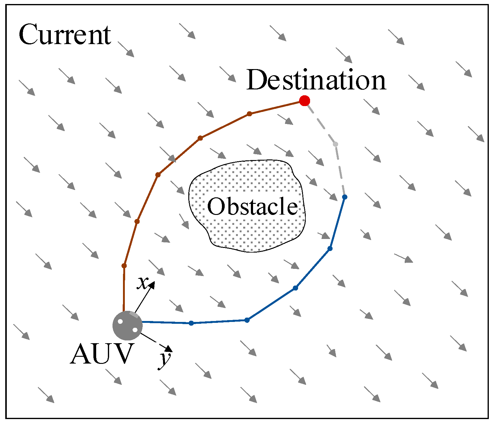
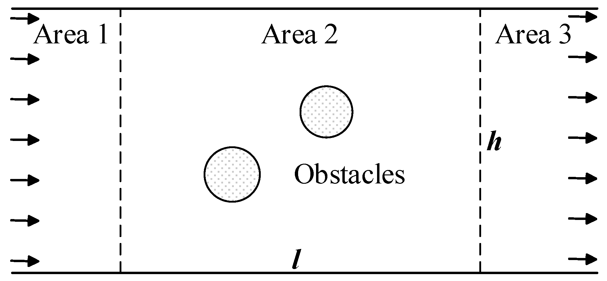
2. Problem Formulation

During operations around underwater structures, the underwater vehicle moves near obstacles according to instructions and avoids collisions. Let $F_R\to {ℝ}^2$ be the configuration space, where obstacles $O_R:\mathcal{A}\to {ℝ}^2$ and time-varying flow fields $\overrightarrow{c}:{\mathcal{D}}_T\to {ℝ}^2$ exist, and ${\mathcal{D}}_T=\mathcal{D}\times [\underset{\_}{t},\overline{t}]$ represent the considered time interval. All positional information within the configuration space $F_R$ is observable. The path planning of the underwater vehicle can be defined as: seeking a reachable and safe route $\epsilon$ from the starting point to the destination in flow field $\mathcal{D}$. The path consists of sub-paths connected by a set of control nodes, denoted as: $\epsilon ={\displaystyle \sum _{i=1}^n{\epsilon }_i},n\in {ℝ}^{+}$.

Let $\overrightarrow{c}$ be the flow speed of the current in the environment and $\overrightarrow{v}$ be the vehicle’s cruising speed in still water; in this case, the vehicle’s actual speed in the environment is:

$${\overrightarrow{v}}^c=\overrightarrow{c}+\overrightarrow{v}$$

(1)

In regions with higher flow velocities within the flow field, we establish the following criteria: if the water flow speed surpasses the vehicle’s velocity, we classify it as a strong current area; otherwise, it is designated as a weak current area. Additionally, we introduce the concept of a mixed flow field; when both strong current and weak current areas coexist in the environment, we refer to this as a mixed flow field.

When the water flow speed exceeds the maximum speed of the AUV, some traditional algorithms may generate paths that include physically infeasible regions. Figure 1 depicts two theoretically feasible solutions obtained using the classical RRT algorithm for the same target point. In one of the paths, the portion against the current exceeds the vehicle’s cruising speed, rendering the path invalid.

For the path planning problem, considering the aforementioned time-varying local flow field, two assumptions are proposed:

Assumption 1. 

The vehicle’s trajectory can be measured or estimated at all time intervals.

Assumption 2. 

The flow field maintains a stable state within a period T, which is greater than the vehicle’s deployment time.

Assessing path quality involves multiple aspects such as path length, time consumption, etc., achieved by designing specific cost functions as optimization goals [15]. In this study, we primarily focus on path length as the main research indicator. Let the path $\epsilon =\{X_1,X_2,\dots X_N\}$ be composed of a set of nodes, where N is the number of nodes. According to the cost function designed by Yan et al. [16], assume the distance cost between adjacent nodes $X_i$ and $X_{i+1}$ is denoted as ${\tau }_i={‖X_{i+1}-X_i‖}_2$, then define our optimization objective function as:

$$\begin{array}{l}\tau ={\displaystyle \sum _{i=1}^{N-1}{\tau }_i}={\displaystyle \sum _{i=1}^{N-1}{‖X_{i+1}-X_i‖}_2}\\ \mathrm{s}.\mathrm{t}.\begin{array}{c}\end{array}{C}_1:X_i\in \mathcal{D}\\ \begin{array}{c}\end{array}\begin{array}{c}\end{array}\begin{array}{c}\end{array}\begin{array}{c}{C}_2\end{array}:X_1=X_{start},X_N=X_{goal}\\ \begin{array}{c}\end{array}\begin{array}{c}\end{array}\begin{array}{c}\end{array}\begin{array}{c}{C}_3\end{array}:t\le \mathcal{T}\end{array}$$

(2)

where, $C_1$ indicates that node $X_i$ must be located within the flow field. $C_2$ signifies that the initial and final points of the function must correspond to the planned starting and target points. $C_3$ denotes that the task duration must fall within the specified time interval.

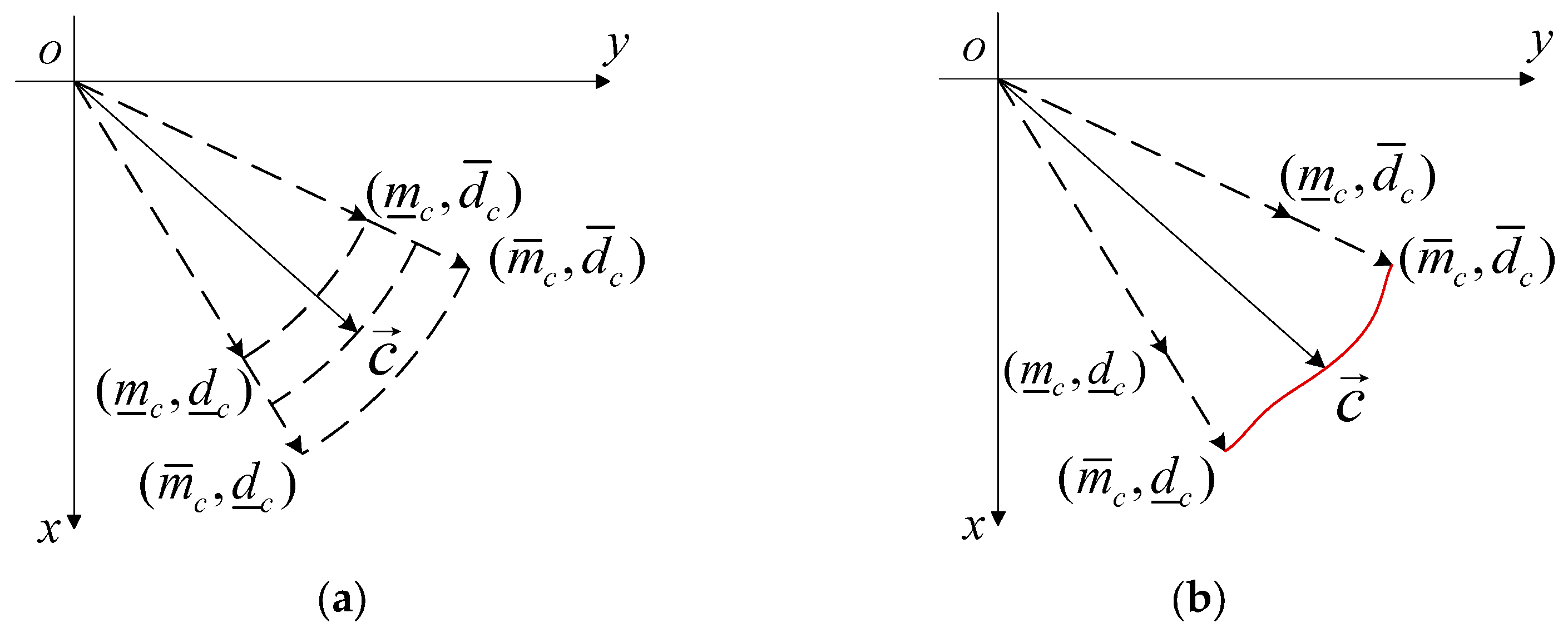
3. Construction of Flow Field Database

The velocity vectors of flow at adjacent grid points are typically similar [17]. Therefore, for flow field $\overrightarrow{c}:{\mathcal{D}}_T\in {ℝ}^2$, assumed to be within the vehicle’s deployment time, it can be divided into a finite number of cells ${\left\{R_i\right\}}_{i\in I_R}$, with the union of all cells constituting the flow field domain $\underset{i\in I_R}{\cup }\{R_i\}=\mathcal{D}$. Let $F_0:\mathcal{D}\times [\underset{\_}{t},\overline{t}]\to {ℝ}^2$ represent the velocity information of all discrete grid points in the flow field within the time interval T. Thus, the velocity information of any cell $R_i$ within the grid is denoted by $\overrightarrow{c}(x,t)=F_0(x,t)$, representing the velocity vector at position x and time $t\in [\underset{\_}{t},\overline{t}]$.

The velocity information can be obtained by predicting historical data of the flow field. For tidal estuaries and oceans, tidal flow prediction models can also be utilized. Due to the presence of errors in prediction data, $\overrightarrow{c}(x,t)$ are not deterministic values. To handle such uncertainty, Yao et al. [18] proposed representing $\forall x\in \mathcal{D}$ and $t\in [\underset{\_}{t},\overline{t}]$ as the flow field, while $\overrightarrow{c}(x,t)=[m_c(x,t),d_c(x,t)]$ represents the magnitude and direction of the velocity vectors, denoted by $m_c(x,t)$ and $d_c(x,t)$, respectively. The uncertainty of the velocity vectors is represented as:

$${\tilde{m}}_c(x,t)\in [{\underset{\_}{m}}_c(x,t),{\overline{m}}_c(x,t)]=[e_m\cdot {\underset{\_}{m}}_c(x,t),(1-e_m)\cdot {\overline{m}}_c(x,t)]$$

(3)

$${\tilde{d}}_c(x,t)\in [{\underset{\_}{d}}_c(x,t),{\overline{d}}_c(x,t)]=[{\underset{\_}{d}}_c(x,t)+e_d,{\overline{d}}_c(x,t)-e_d]$$

(4)

where $\tilde{\bullet }$ represents the uncertainty of the variable $\bullet$, the boundary values of the velocity vector interval are determined by the maximum and minimum values predicted from multiple forecasts, and $e_m$ and $e_d$ are coefficients.

Consider that when ${\underset{\_}{m}}_c\le v\le {\overline{m}}_c$, this indicates that the vehicle’s maximum speed lies within the range of velocity variations, leading to a probability of rendering the path infeasible. Improving Equation (3), we have:

$$m_c(x,t)=m_{\max }(x,t,d_c)=(1-e_m)\cdot {\overline{m}}_c(x,t,d_c)$$

(5)

where $d_c$ represents the direction angle of the current. The flow field can be expressed as:

$$\left\{\begin{array}{l}{m}_c(x,t)=m_{\max }(x,t,d_c)=(1-e_m)\cdot {\overline{m}}_c(x,t,d_c)\\ d_c(x,t)\in [{\underset{\_}{d}}_c(x,t),{\overline{d}}_c(x,t)]=[{\underset{\_}{d}}_c(x,t)+e_d,{\overline{d}}_c(x,t)-e_d]\end{array}\right.$$

(6)

Figure 2 provides a comparison between two methods of expression, where the difference lies in the value selection of the velocity scalar. The expression proposed in this paper takes the maximum value of velocity while keeping the angle interval unchanged, aiming to mitigate the risk of infeasible paths.

According to the current information of the environment, a field database can be constructed using the improved Equation (6). To obtain the current information, a combination of ROMS and CFD is adopted in this paper, which is divided into the following two scenarios:

Case 1: Free areas far from obstacles including area 1 and area 3, which is shown in Figure 3. Information of such areas is obtained from ROMS and serves as guidance information for CFD simulation.

Case 2: Areas near obstacles, as shown in Figure 3, area 2. Influenced by specific obstacle boundaries, these areas exhibit greater flow field gradients, with localized increases in velocity, reduced flow, or turbulence. Information about such areas is obtained from CFD simulation.

Research on numerical simulations of river flow fields have been conducted by scholars, yielding a series of achievements in hydrodynamics and flow field characteristics [19,20]. In tidal estuaries or nearshore areas, a complete tidal history dataset can serve as boundary conditions for simulations. By establishing a simulation database at given time intervals (T), based on a complete tidal cycle, this process can be conducted as preliminary work on a PC before deploying vehicles. Combined with the flow field database and the path planning method, the main structure of the algorithm in this paper is shown in Figure 4:

4. Directed Expansion Method of Path

Consider a local trajectory $\stackrel{\rightharpoonup }{d}$ in the current $\overrightarrow{c}$ over a time interval T. Equation (1) leads to the inference: $\overrightarrow{d}=\overrightarrow{c}+{\overrightarrow{v}}^c$. Let $\theta \in [-\mathrm{\pi },\mathrm{\pi }]$ denote the angle between the vehicle’s heading direction and current, and $c^d$ represents the angle between the trajectory $\stackrel{\rightharpoonup }{d}$ and current. According to the cosine rule of triangles, the relationship between $c^d$ and $d$ is derived as follows:

$$\cos c^d={\displaystyle \frac{c^2+d^2-v^2}{2cd}}$$

(7)

where the range of $d$ is $\left|c-v\right|\le d\le c+v$, based on the relationship of triangle lengths. By giving the values of $v$ and $c$ under different directional angles, three cases are discussed as follows:

Proof. 

Case 1: $c=v$. Where the magnitude of current speed equals the magnitude of the vehicle’s cruising speed and the range of d becomes [0, 2c]. Thus, Equation (7) is updated:

$$\cos c^d={\displaystyle \frac{d}{2c}},c=v$$

(8)

which leads to the relationship that $c^d$ is directly proportional to the variable $d$. We can solve this relationship to yield the range of values for $c^d$ as $\left[-\mathrm{\pi }/2,\mathrm{\pi }/2\right]$. From a geometric perspective, the feasible range of $\overrightarrow{d}$ lies within the same half-plane as $\overrightarrow{c}$, as illustrated in Figure 5a.

Case 2: $c>v$. The range of $d$ is $\left[c-v,c+v\right]$. Thus, rewriting Equation (7) with $d$ as the independent variable, we have:

$$\cos c^d={\displaystyle \frac{c^2+d^2-v^2}{2cd}}={\displaystyle \frac{1}{2c}}\left(d+M\right)$$

(9)

which is an odd function with respect to $d$, and $M={\displaystyle \frac{c^2-v^2}{d^2}}$. Let $f(d)={\displaystyle \frac{1}{2c}}(d+M)$. Taking its derivative reveals:

$$f^{\prime }(d)={\displaystyle \frac{1}{2c}}\left(1-M\right)$$

(10)

Due to $0\le c-v\le d\le c+v$, we know that $f(d)$ attains its minimum value at $d=\sqrt{c^2-v^2}$, thus:

$$f(d)\ge f(\sqrt{c^2-v^2})=Q$$

(11)

where $Q={\displaystyle \frac{\sqrt{c^2-v^2}}{c}}$. From the above equation, it is understood that the range of $\cos c^d$ is $\left[Q,1\right]$, which implies the range of angle $c^d$ is $c^d=\left[-\arccos Q,\arccos Q\right]$. As illustrated in Figure 5b, the feasible range lies within the sector along the direction of water flow.

Case 3: $c<v$. We have $c^2-v^2<0$, thus the range of $d$ is $\left[v-c,c+v\right]$. Similar to the derivation in case 2, Equation (10) should be rewritten as:

$$f^{\prime }(d)={\displaystyle \frac{1}{2c}}\left(1+M\right)>0$$

(12)

It is evident that the function is a monotonically increasing function, meaning that $f(v-c)\le f(c^d)\le f(c+v)$. The range of $c^d$ is determined to be $\left[-\mathrm{\pi },\mathrm{\pi }\right]$. As illustrated in Figure 5c, the feasible range in this case is complete. □

The analysis above addresses the feasibility between current velocity and vehicle cruising speed under three distinct relationships. We know that when the cruising speed surpasses the water flow velocity, the vehicle can move freely along any angle, effectively overcoming the water flow’s influence. Conversely, there exist infeasible angles. When the cruising speed is lower than the current velocity, the infeasible range is determined by the magnitude of current velocity. In line with the rationale outlined in the first section of this chapter, the velocity vectors of the uncertain flow field fluctuate within a specific range. To ensure the path’s feasibility at any given instance, the intersection of all feasible ranges within this interval is selected as the actual feasible range of the uncertain flow field, which is expressed as follows:

$$\omega ={\underset{\_}{c}}_d(x,t)\cap {\overline{c}}_d(x,t)$$

(13)

When the node is located at different positions of the cell, the total feasible range of the node depends on the number of its adjacent cells. As shown in Figure 6a, for node $X_i$, it has n (n = 1, 2, 3, 4) adjacent cells; in this case, the feasible range is:

$${\omega }_i=\left\{\begin{array}{l}{\omega }_n,n=1\\ {\displaystyle \sum _{x=1}^n{\omega }_x,}\hspace{0.33em}n=2,3,4\end{array}\right.$$

(14)

Therefore, nodes situated on the boundary often possess a broader feasible range than those within the cell. The expansion method of the path is shown in Figure 6b. For node $X_i$, the feasible range ${\omega }_i$ is discretized into k possible moving directions. Then the node that the AUV can reach in the next step is $X_{i+1}=\{X_{i+1}^0,X_{i+1}^1\dots X_{i+1}^n\}$, and the path containing the target point $X_{goal}$ is a feasible solution.

5. Path Planning in Mixed Flow Fields

In this section, we aim to address the feasibility and efficiency challenges of AUV path planning in strong currents environments, design a path planning method according to the database construction method and feasibility analysis presented in the previous two sections. A hierarchical planning strategy has been devised, comprising an enhanced RRT-based method for swift convergence in global planning, and a local path correction approach. Each component of the algorithm will be discussed individually.

5.1. Standard RRT Algorithm

The standard RRT algorithm is adept at handling nonholonomic constraints, including dynamics, and high degree of freedom (DOF) problems [21]. By iteratively expanding the RRT using control inputs, as illustrated in Figure 7, the system is guided toward randomly selected points. The sampling-based expansion method ensures that the sampled vertices approximate a uniform distribution and is theoretically probabilistically complete. However, the initial paths generated by the RRT algorithm cannot be directly applied to the vehicle’s motion trajectory due to the following drawbacks:

(1) The initial path is not optimal and can be further optimized in conjunction with dynamic constraints.

(2) In the later stages of RRT expansion, as well as in regions with narrow passages, the growth rate of the tree is slow, resulting in low exploration efficiency.

The sampling-based search approach of RRT, compared to methods requiring grid map construction, offers higher search efficiency [22]. Utilizing the path planned by RRT as an initial solution, and conducting secondary optimization to obtain better results, is a settlement that possesses both efficiency and path quality.

5.2. Hierarchical Path Planning Algorithm

We propose an optimization algorithm called Curtate-RRT(C-RRT), which requires obtaining a feasible initial solution ${\epsilon }_0:[0,x]\to {ℝ}^2$ first. The solution, which is comprised of a finite number of nodes with a fixed distance of $d$, is derived from the standard RRT algorithm. ${\epsilon }_t$ represents the path optimized after $t$ iterations. The optimization process of the algorithm consists of two key components. The first part involves sampling within the global scope to obtain a feasible theoretical optimal solution, which includes two main modules: path contraction and corner point optimization. The second part involves feasibility checking of the theoretical optimal solution. If there are infeasible parts, local corrections are made through directed expansion. The pseudocode of the algorithm is as follows:

In Algorithm 1, the initial phase (from line 1 to line 11) mirrors the steps of the RRT algorithm. It begins by randomly sampling a point $X_{rand}$ from the workspace $S$, then searches for the nearest node $X_{nearst}$ on the tree to $X_{rand}$ and creates a new point $X_{new}$ at a fixed step length. Collision detection is applied to $X_{new}$, and if no collision is detected, it is added to the tree, and its parent node is recorded. Using a threshold $\delta \in {ℝ}^{+}$, the algorithm calculates the Euclidean distance $\Delta d=‖X_{goal}-X_{new}‖$ between the target point $X_{goal}$ and $X_{new}$. If $\Delta d\le \delta$, the target point is deemed reached. The function $T\leftarrow LineCurate(X_{start},X_{goal},T,obstacle)$ (line 13) is the path shrinkage module, which refines the initial solution to a transitional one that tightly hugs obstacles. This process concludes swiftly. Following this, the corner optimization module iteratively optimizes the corner points of the new path until the optimal solution is obtained. Line 18 to line 20 handle local path correction; if any infeasible sections are encountered, $T\leftarrow LocalRewise(S,T,obstacle)$ (line 19) is executed for local replanning. Otherwise, the program concludes and returns the planning result.

Algorithm 1: C-RRT

Data: Xstart, Xgoal, workspace S, obstacle    Result: T 1 $V\leftarrow X_{start};$ 2 $E\leftarrow 0;$ 3 $T\leftarrow (V,E);$ 4 for $iteration=1\dots n$ do 5  $X_{rand}\leftarrow Sample(X_{start},X_{goal},S);$ 6  $X_{nearest}\leftarrow Nearest(X_{nearst},X_{rand});$ 7  $(X_{new},X_{parent})\leftarrow Steer(X_{nearst},X_{rand});$ 8  if $\mathit{CollisionFree}\left(X_{\mathit{nearst}},X_{\mathit{new}},\mathit{obstacle}\right)$ then 9         $V\leftarrow V\cup \left\{X_{new}\right\};$ 10        $T\leftarrow T\cup \{X_{new},X_{parent}\};$ 11         if $\parallel X_{\mathit{new}}-X_{\mathit{goal}}\parallel \le q$ then 12              $V\leftarrow V\cup \left\{X_{goal}\right\};$ 13                      $T\leftarrow LineCurtate\left(X_{start},X_{goal},T,obstacle\right);$ 14              $T\leftarrow AngleOptimization(X_{start},X_{goal},T,obstacle);$ 15        end 16  end 17  $iteration\leftarrow iteration+1;$ 18  if $\mathit{AccessibilityCheck}{\displaystyle (T,S)}$ then 19        $T\leftarrow LocalRewise(S,T,obstacle);$ 20    end 21  end 22 return $V$

A.

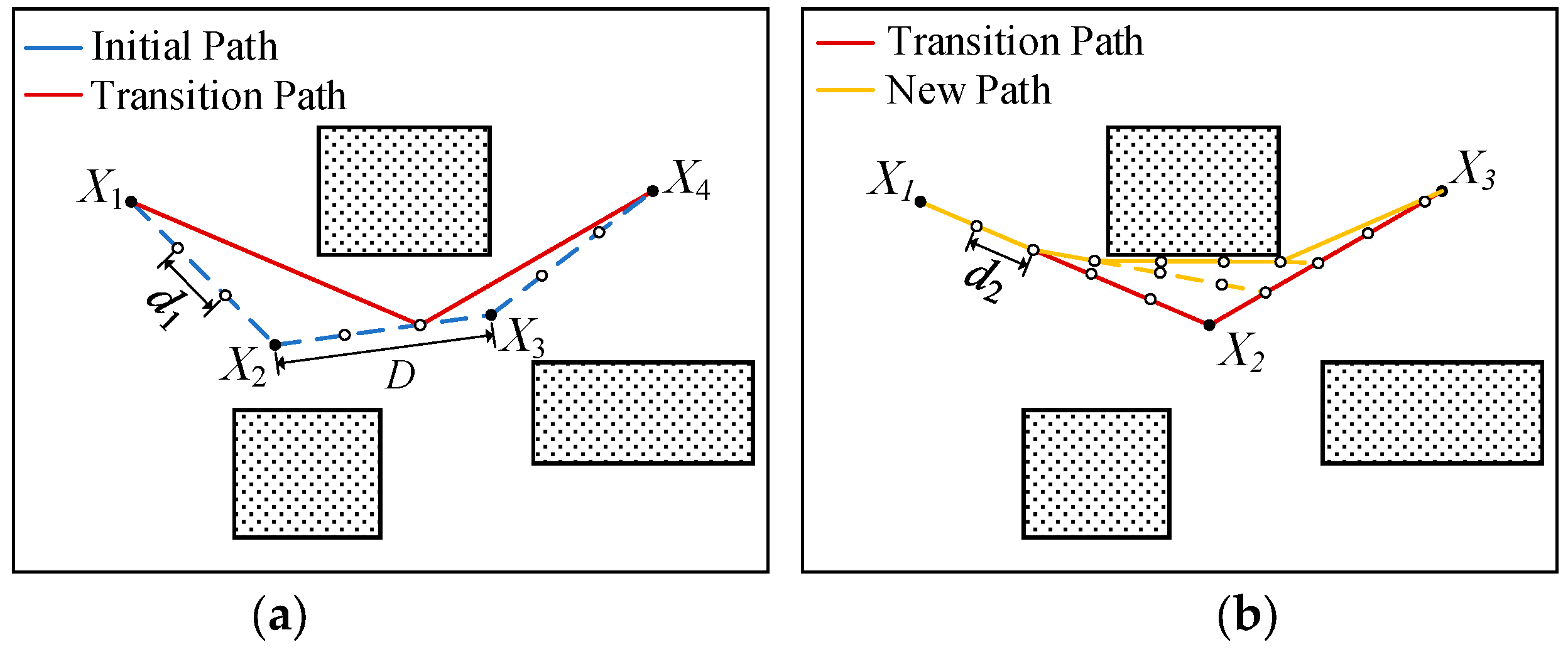
Path shrinkage

Between adjacent nodes $X_i$ and $X_{i+1}$, interpolate uniformly with a step length $d_1$, and add newly generated points to the set of path points ${\dot{X}}_s(x,y)\in {\epsilon }_t,(s=1,2,\dots ,n)$, where $d_1<d$. Reorder the new point sets sequentially. As shown in Figure 8a, from the starting point $X_{start}$, all remaining visible nodes are connected in each iteration, with collision detection performed during each connection attempt. The last node without collision is taken as the next starting point, and the process continues until reaching the target point $X_{goal}$.

B.

Corner optimization

Let $X_i(x,y)$ be any node except the starting and ending points. Given a midpoint $X_i$, the previous node $X_{i-1}$ is denoted as the left node, and the succeeding node $X_{i+1}$ is termed the right node. As shown in Figure 8b, using step size $d_1$, interpolate equidistantly along the line segments $\overline{X_{i-1}{X}_i}$ and $\overline{X_i{X}_{i+1}}$, preceding and succeeding point $X_i$ respectively, resulting in two interpolated point sets ${\dot{X}}_{i-1}(t),(t=1,2,\dots ,n)$ and ${\dot{X}}_i(t),(t=1,2,\dots ,n)$. For the point set ${\dot{X}}_i(t)$, starting from the initial point, sequentially connect ${\dot{X}}_i(t)$ with all points in another set ${\dot{X}}_{i-1}(t)$, performing collision detection with each connection until a collision occurs. The node ${\dot{X}}_{i-1}(t)$ just before the collision becomes the left node, while ${\dot{X}}_i(0)$ becomes the middle node. Repeat the previous steps for line segments $\overline{{\dot{X}}_{i-1}(t){\dot{X}}_i(0)}$ and $\overline{{\dot{X}}_i(0)X_{i+1}}$ until the middle node overlaps with the right node; then, the search ends. The shortest path after segmentation represents the optimized path.

C.

Local path correction

When the velocity of current is low, the first two steps can complete the planning task. When strong flow exists in the flow field, further optimization of this step is required. This step is derived from the theoretical analysis in Section 3, and uses a directed search method to correct the feasibility of the path.

After systematically examining the current information in each grid cell along the path, it is determined whether or not the path enters a strong current zone. If it does not pass through a strong current zone, the algorithm terminates; otherwise, the entry point $S_0$ and exit point $S_n$ of the strong current zone are identified. For the segment within the strong current zone, the flow field grid cells are sequentially checked to determine if the path direction falls within the feasible range of the grid cell. The analysis is conducted under the following two cases:

Case 1: The path direction entirely aligns with the feasible range of the grid cell. In such instances, the path is deemed a feasible optimal solution, and the algorithm concludes.

Case 2: There are segments of the path that deviate from the feasible range of the grid cell. In this case, with $S_0$ and $S_n$ as the starting and target points, respectively, the reachable point set $\{S_1,\dots S_n\},n\in {ℝ}^{+}$ for the next step is recorded. Each point in the set is examined sequentially to identify the next reachable point set. Nodes beyond the boundaries of the strong current zone are disregarded. Upon the appearance of the target point in the reachable point set, a feasible solution is deemed to be found. After traversing all potential solutions, the shortest one is selected as the final solution, and the algorithm concludes.

5.3. Algorithm Analysis

To test the path quality near obstacles, a group of scenarios containing different obstacles were selected for comparative testing. As shown in Figure 9, the RRT path is the initial path and the C-RRT path is the optimized result of initial path. The optimized path has good adaptability to both circular and rectangular boundaries. As for the sharp turning points in the initial path, there are no sharp corners in the path after optimization.

Concerning the primary parameter influencing algorithm efficiency, the discrete step size d₂, we examined the variation trend of path length and time cost for different values, as depicted in Figure 10. The segments lacking data indicate planning failures, which is attributed to a significant surge in computational work upon the reduction of step size, thus resulting in planning times surpassing the set threshold. Once the step size dips below 0.3, the rate of distance change remains below 5%, while the rate of increase in time cost exceeds 200%. Therefore, to improve the efficiency of the algorithm, the step size cannot be too small, which means that path quality needs to be lost partially.

Local path correction entails rectifying infeasible paths in the strong current zones. Beginning from the entry point into the strong current zone, a directed search can yield a finite number of reachable paths to the exit point. Since the weak current zones have complete feasible ranges, the boundaries between the weak and strong current zones must constitute feasible paths. This study reduces computational costs compared to search algorithms based on grid maps by exclusively searching within the strong current zones.

6. Example Study

In this chapter, we conducted simulation experiments employing the proposed flow field modeling and path planning methods. First, we described the parameter settings for the reference experimental environment and simulation experiments to establish the flow field database. Subsequently, we subjected the method presented in this paper to simulation experiments based on the data from the flow field model and compared its performance with other path planning methods.

6.1. Simulation Parameter Settings

The reference environment is the estuary of the Minjiang River in Fujian Province. Flow field around the bridge piers is selected as the CFD simulation area, with the size 50 m × 50 m. The bridge pier diameter is 1.2 m, and the distance between adjacent piers is 6 m. As a tidal estuary, the local water velocity obtained from ROMS ranges from 0.2 m/s to 1.4 m/s. These tidal currents serve as input velocity information for the numerical simulation of this flow field. CFD calculations are performed using Ansys/Fluent 2022R1 software to obtain initial simulation data. The turbulence model adopted is the $k-\omega$ model. An unstructured grid is used for computing. Simulations are conducted at speed intervals of 0.15 m/s. For each velocity level, ten simulations are performed under the same environmental conditions, and the current data are generated using the flow field uncertainty formula. The region where the water flow velocity exceeds the vehicle’s sailing speed is identified as the strong current.

The algorithm-related parameter settings are: initial step size D of RRT is 5 m, optimization algorithm d₁ and d₂ are 1 and 0.5, respectively. The parameter settings for AUV: maximum speed V_max = 1.5 m/s. As the algorithm does not involve the dynamics of AUV, parameters about dynamics are not designed. In practical algorithm deployment, constraints such as vehicle’s collision avoidance distance also need to be considered.

6.2. Result of Path Planning

Figure 11 illustrates a planning example employing the algorithm proposed in this paper. Result is shown at a 20 m × 14 m rectangular area, with a maximum travel time limit of 5 min, juxtaposing the planning outcomes across diverse task scenarios. Furthermore, the computational outcomes of the proposed C-RRT algorithm are contrasted with those of RRT* and A*.

Table 1. Comparison of path planning results.

	Length (m)		Time (s)		Corner
	Task a	Task b	Task a	Task b	Task a	Task b
RRT*	32.3	31.7	48	47	7	6
C-RRT	28.2	35.3	32	40	3	3
A*	26.1	26.3	55	56	3	12

offers a comprehensive comparison of the three algorithms across different dimensions, including time and path distance.

It can be observed that in the downstream direction, the paths planned by all three methods exhibit no feasibility issues. CRRT achieves the shortest computation time among the three algorithms, while slightly lagging behind A* in terms of path length. This indicates that even after sacrificing some path quality, the resulting paths still perform well, with CRRT demonstrating an advantage in computation time. In the upstream direction, due to the absence of consideration for the impact of strong water currents on the vehicle, both RRT* and A* exhibit some infeasible sections. The algorithm proposed in this paper incurs additional costs in distance when circumventing strong current zones. However, it still outperforms the other two algorithms in terms of computation time. This is because A* requires traversing a large number of grid cells during expansion, while RRT* needs numerous iterations to approach the optimal solution. In contrast, C-RRT only needs to traverse cells in the strong current zone, thus saving some ineffective computation time.

From Figure 11 and Table 1, the following conclusions can be drawn: the path planning method proposed in this paper is suitable for local scenarios such as river channels and nearshore areas with dynamic water flow. However, in large-scale flow fields, actual water flow is influenced by numerous factors, leading to significant deviations from numerical simulation results and reduced effectiveness of the outcomes. For all applicable flow fields, obtaining approximate hydrological conditions of the environment is crucial for establishing preprocessing. Additionally, the actual planning effectiveness is constrained by the vehicle’s dynamics and control input capabilities. Due to the discrepancies between the simulation environment and the real environment, it is necessary to consider the uncertainty of simulated flow fields. For predicting flow velocities within the flow field domain, future research could explore time-series prediction based on historical data. Furthermore, further strategic analysis can be conducted regarding the different angles between vehicle heading and water flow direction.

7. Conclusions

In actual operational scenarios, the navigation of small AUVs is significantly influenced by water currents, making accurate flow field information crucial for vehicle motion control. This paper conducts numerical simulations of specific scenarios based on Computational Fluid Dynamics (CFD) and ocean current prediction data, constructing a flow field database. A special focus is placed on analyzing areas of strong currents where the flow velocity exceeds the vehicle’s sailing speed. Subsequently, research on underwater vehicle path planning is conducted. A feasible and efficient hierarchical path planning strategy is designed and analyzed in detail, with theoretical analysis and simulations confirming the feasibility of the algorithm.

In the study, numerical simulation is performed under two-dimensional plane assumptions. In future work, a more complicated three-dimensional flow field will be studied to provide a more practical and accurate numerical simulation, which assists in the path planning of underwater vehicles. Moreover, since some underwater activities or harsh marine environments affect the autonomy, propulsion performances, and maneuverability of underwater vehicles [23], the mapping of underwater vehicle performance with respect to current will be studied.

References

- Cheng, C.; Sha, Q.; He, B.; Li, G. Path planning and obstacle avoidance for AUV: A review. Ocean Eng. 2021, 235, 109355. [Google Scholar] [CrossRef]
- Zhu, D.; Yang, S.X. Path planning method for unmanned underwater vehicles eliminating effect of currents based on artificial potential field. J. Navig. 2021, 74, 955–967. [Google Scholar] [CrossRef]
- Soulignac, M. Feasible and optimal path planning in strong current fields. IEEE Trans. Robot. 2010, 27, 89–98. [Google Scholar] [CrossRef]
- Kruger, D.; Stolkin, R.; Blum, A.; Briganti, J. Optimal AUV path planning for extended missions in complex, fast-flowing estuarine environments. In Proceedings of the IEEE International Conference on Robotics and Automation, Rome, Italy, 10–14 April 2007; IEEE: Piscataway, NJ, USA, 2007; pp. 4265–4270. [Google Scholar]
- Vasudevan, C.; Ganesan, K. Case-based path planning for autonomous underwater vehicles. Auton. Robot. 1996, 3, 79–89. [Google Scholar] [CrossRef]
- Zhu, D.; Yang, S.X. Bio-inspired neural network-based optimal path planning for UUVs under the effect of ocean currents. IEEE Trans. Intell. Veh. 2021, 7, 231–239. [Google Scholar] [CrossRef]
- Chu, Z.; Wang, F.; Lei, T.; Luo, C. Path planning based on deep reinforcement learning for autonomous underwater vehicles under ocean current disturbance. IEEE Trans. Intell. Veh. 2022, 8, 108–120. [Google Scholar] [CrossRef]
- Lefebvre, N.; Schjølberg, I.; Utne, I.B. Integration of risk in hierarchical path planning of underwater vehicles. IFAC-Pap. 2016, 49, 226–231. [Google Scholar] [CrossRef]
- Miotto, P.; Wilde, J.; Menozzi, A. UUV on-board path planning in a dynamic environment for the Manta test vehicle. In Proceedings of the Oceans 2003. Celebrating the Past… Teaming Toward the Future (IEEE Cat. No. 03CH37492), San Diego, CA, USA, 22–26 September 2003; IEEE: Piscataway, NJ, USA, 2003; Volume 5. [Google Scholar]
- Wang, K.; Li, S.; Wang, Y.; Xi, J. Smooth-RRT*: An Improved Motion Planner for Underwater Robot. In Proceedings of the 2022 27th Asia Pacific Conference on Communications (APCC), Jeju Island, Republic of Korea, 19–21 October 2022; IEEE: Piscataway, NJ, USA, 2022. [Google Scholar]
- Chowdhury, M.I.; Schwartz, D.G. USV Obstacle Avoidance Using a Novel Local Path Planner and Novel Global Path Planner with r-PRM. In Proceedings of the ISR Europe 2022; 54th International Symposium on Robotics, Munich, Germany, 20–21 June 2022; VDE: Berlin, Germany, 2022. [Google Scholar]
- Heo, Y.J.; Chung, W.K. RRT-based path planning with kinematic constraints of AUV in underwater structured environment. In Proceedings of the 2013 10th International Conference on Ubiquitous Robots and Ambient Intelligence (URAI), Jeju, Republic of Korea, 30 October–2 November 2013; IEEE: Piscataway, NJ, USA, 2013. [Google Scholar]
- Yu, L.; Wei, Z.; Wang, Z.; Hu, Y.; Wang, H. Path optimization of AUV based on smooth-RRT algorithm. In Proceedings of the 2017 IEEE International Conference on Mechatronics and Automation (ICMA), Takamatsu, Japan, 6–9 August 2017; IEEE: Piscataway, NJ, USA, 2017. [Google Scholar]
- Shchepetkin, A.F.; McWilliams, J.C. The regional oceanic modeling system (ROMS): A split-explicit, free-surface, topography-following-coordinate oceanic model. Ocean Model. 2005, 9, 347–404. [Google Scholar] [CrossRef]
- Hou, M.; Cho, S.; Zhou, H.; Edwards, C.R.; Zhang, F. Bounded cost path planning for underwater vehicles assisted by a time-invariant partitioned flow field model. Front. Robot. AI 2021, 8, 575267. [Google Scholar] [CrossRef] [PubMed]
- Yan, Z.; Zhao, Y.; Zhang, H. A method of UUV path planning with biased extension in ocean flows. In Proceedings of the 10th World Congress on Intelligent Control and Automation, Beijing, China, 6–8 July 2012; IEEE: Piscataway, NJ, USA, 2012; pp. 532–537. [Google Scholar]
- Hao, K.; Zhao, J.; Li, Z.; Liu, Y.; Zhao, L. Dynamic path planning of a three-dimensional underwater AUV based on an adaptive genetic algorithm. Ocean Eng. 2022, 263, 112421. [Google Scholar] [CrossRef]
- Yao, X.; Wang, F.; Yuan, C.; Wang, J.; Wang, X. Path planning for autonomous underwater vehicles based on interval optimization in uncertain flow fields. Ocean Eng. 2021, 234, 108675. [Google Scholar] [CrossRef]
- Wang, Y.; Liu, Y.; Miao, G. Three-dimensional numerical simulation of viscous flow around circular cylinder. J. Shanghai Jiaotong Univ. 2001, 35, 1464–1469. [Google Scholar]
- Yang, W.L.; Wu, C.W.; Zhu, Q.L.; Wang, G. Refined study on 3D flow characteristics around bridge piers. J. Southwest Jiaotong Univ. 2020, 55, 134–143. [Google Scholar]
- LaValle, S. Rapidly-exploring random trees: A new tool for path planning. Res. Rep. 9811 1998. Available online: https://lavalle.pl/papers/Lav98c.pdf (accessed on 19 November 2024).
- Kim, J.T.; Li, J.H.; Lee, M.J.; Kim, J.G.; Suh, J.H. Path planning for uncertainty reduced monitoring. In Proceedings of the OCEANS 2014-TAIPEI, Taipei, Taiwan, 7–10 April 2014; IEEE: Piscataway, NJ, USA, 2014; pp. 1–6. [Google Scholar]
- Pugi, L.; Pagliai, M.; Allotta, B. A robust propulsion layout for underwater vehicles with enhanced manoeuvrability and reliability features. Proc. Inst. Mech. Eng. Part M J. Eng. Marit. Environ. 2018, 232, 358–376. [Google Scholar] [CrossRef]