Operation Analysis of the Floating Derrick for Offshore Wind Turbine Installation Based on Machine Learning

Abstract

To investigate the influencing factors on the operation of an offshore wind turbine installation ship, a neural network, as a machine-learning method, is built to predict and analyze the motion response of a floating derrick in the process of a lifting operation under an external environmental load. The numerical method for the double floating body, from the software SESAM/SIMA, is validated against the experiments. The numerical method is used to establish the floating derrick-lifting impeller model to obtain the motions of the ship and impeller and the coupling effect. Based on the numerical results, the BP neural network model is built to predict the ship’s operation. The results show that the BP neural network model for the floating derrick and impeller motion prediction is very feasible. Combined with the Rules for Lifting Appliances of Ships and Offshore Installations and the Noble Denton Guidelines for Marine Lifting Operations, the operation of the floating crane system can be determined based on the environmental parameters.

1. Introduction

Since the mid-1960s, researchers have integrated knowledge from various disciplines into the component structure learning system method to better simulate the human learning process. Over the years, significant progress has been made in many areas. With the development of computers, electronic sensing, and other related technologies, intelligent equipment data on ships can realize real-time monitoring and storage of motion data on hull operations. Analyzing this data using machine-learning techniques offers valuable insights for optimizing installation and construction processes, ultimately improving production efficiency. This represents the future direction of the shipbuilding industry [1].

Machine learning can be divided into supervised learning, unsupervised learning, semi-supervised learning, and reinforcement learning, according to different tasks. The core goal of the supervised-learning algorithm is to learn a model or function to map the input to the correct output. This model is usually called a classifier or regression. Using machine-learning technology to analyze the hull dimension, the actual research is on the relationship between the dependent variable (target) and the independent variable (predictor). A regression model is a relatively simple predictive modeling technique in machine learning. The relationship between the length, width, draught, ship mass, and maximum load of the same type of ship was obtained using the regression analysis by Kristensen [2]. It can not only illustrate the significant relationship between independent variables and dependent variables but also the influence intensity of multiple independent variables on a dependent variable by comparing the interaction between variables. The main dimensions of many ship types were determined by a series of non-linear regressions using the deadweight as the input parameter, and a regression formula was proposed for estimating the main dimensions of the container ship by Papanikolaou [3]. With the development of the ship and the increase in the carrying capacity, the regression formula of the past ship type as the learning object has deviated. At the same time, with the development of machine learning, new regression methods have gradually matured and been applied to ship technology. The length, width, and draft depth of a ship were predicted using the maximum load capacity and design speed of the ship as input by an artificial neural network (ANN) [4]. After training, the average absolute error of the model was 4.552%, which can predict the parameters of the ship well. After that, a preliminary design formula was developed using the container ship database established by an ANN in 2015 [5]. The multivariate nonlinear regression with a random search function is used to establish the model, which is as accurate as the estimation created by ANN. It is shown that multi-input parameters can improve the estimation accuracy compared to single-input parameters.

Except for ship design, machine learning has many applications in the field of ship and ocean engineering. Based on a large amount of data in intelligent ships, an ANN-accurate regression model is proposed for main engine fuel consumption by Jeon et al. [6]. By changing the number of hidden layers and neurons and combining different types of activation functions, the influence of hyper-parameters on the regression analysis was compared and analyzed. The results show that the model has a better prediction of main engine fuel consumption, and its accuracy is higher than that of support vector machine prediction. The prediction of aircraft carrier motion response was investigated using the convolution method by Kaplan [7]. Subsequently, Kalman filtering [8], wavelet analysis [9], and time series analysis [10] were focused on by the scholars. Compared with the prediction methods mentioned above, an artificial neural network has strong nonlinear mapping and self-learning ability, with the advantages of high-speed optimization. The rules between the data can be found independently, and finally, the expected output can be obtained through the rules, eliminating the process of treating the data and establishing the model. It has become a research hotspot in recent years. Based on the long-term prediction ability of the recurrent neural network, the multi-step advanced prediction under a hybrid learning strategy was performed in the form of the multi-stage prediction of Li et al. [11]. An online real-time ship attitude prediction model was established based on a long-term and short-term memory artificial neural network [12], which was suitable for online parameter adjustment. The AR (autoregressive)-EMD (empirical mode decomposition)-SVR (support vector regression) model was proposed by combining the SVR [13], which can predict the very short time motion of the ship as pitch and heave. The results show that the multi-algorithm combined model has a higher accuracy. Through a multi-layer artificial neural network, the motion of the ship can be predicted in the next 7 s with high precision by combining the singular value and the genetic algorithm [14].

In the process of a floating crane lifting at sea, the ship’s hull and lifting objects will induce a coupling motion with each other, including the crane, hull, boom, and other components in the system, which makes the overall motion of the system nonlinear. Researchers have made many attempts to study the lifting motion response. Based on the theory of multi-body dynamics, the six-degrees-of-freedom motion equations of the floating crane and the suspended object were established, respectively, by Cha et al. [15], by which the dynamic process of the floating crane lifting large-weight objects was simulated under the different wave heights and frequencies. A complete physical model of a floating crane-suspended object was established by Van Trieu [16], considering the disturbance caused by seawater’s viscoelasticity, suspension wire rope elasticity, and ship-induced motions. A controller was designed to manage the system response well. To investigate the influence of the environment and lifting parameters on the response, the simulation calculation model of the floating crane was established by considering the coupling effect between the mooring system and the lifting system using numerical methods based on the BEM and FEM [17]. The influence of suspended load, waves, crane swings, vessel draft, and mooring tension were analyzed. A model of a floating crane ship was tested to study the motion response obtained in the lifting process [18]. The coupled motion responses of a floating crane vessel and a lifted subsea manifold were investigated during deep-water installation operations. At the same time, big-data and machine-learning algorithms have been applied by researchers. Taking advantage of shrinkage models, such as Ridge and Lasso, the relationship between the features was learned from the original data. A methodical approach based on statistical learning was presented to model the ship performance monitoring problem by Omer Soner el. [19]. It was capable of increasing the situational awareness of ship operators and monitoring ship performance. An optimization method for dual-crane collaborative lifting was proposed with the goal of minimum energy consumption by An et al. [20]. By utilizing data analysis techniques, including clustering algorithms and neural networks, predictive models were established [21]. The models can explore trailing suction hopper dredgers’ energy efficiency deeply, optimize their energy management, enhance operational efficiency, and provide technical support for the intelligent and green development of the maritime industry. The ship energy consumption was analyzed using Python as a data-mining tool [22] to analyze the relationship between energy efficiency parameters and fuel consumption, which provided a reference for energy efficiency management-related decisions.

As more and more offshore wind farms are built in China, the cost needs to be reduced without subsidy from the government. This will result in a reduction of the installation cost, including the engineering ship cost, cargo ship cost, and so on. To reduce the cost of the floating derrick, as the main engineering ship, it is necessary to investigate the operation. However, there is no detailed data analysis and research on the operation of offshore wind turbine installation ships in China. Therefore, it is crucial to identify the influencing factors of the operation of a floating derrick. Due to complex environment loads and the nonlinear response of the ship, the machine-learning method as a BP neural network can be used to predict and analyze the motion response of the floating derrick and the lifting objects. Based on this, the efficiency of offshore wind turbine lifting operations is improved, which will reduce the cost of offshore wind power installation.

During the offshore wind turbine installation process, the floating crane system, which consists of the derrick, lifting objects, and cargo ship, functions as a coupled system. The ship’s motion induces additional movement in the lifted object, while the object’s motion, in turn, affects the ship’s stability. This system is significantly influenced by the complex external marine environment, including waves, wind, and currents. In addition, throughout the operation, the lifting height, crane position, and the center of gravity of the crane–impeller system dynamically changes as the crane rotates.

In this paper, an analysis of the impact of environmental factors and lifting parameters on the system’s motion response will be conducted to predict the operation of the floating crane system. The lifting of the impeller by the floating derrick is specifically examined. The numerical predictions using the software SESAM/SIMA [23] of the motion responses of the two barges in double floating body system are validated against experiments in regular and irregular conditions first. The numerical method is then used to establish the floating derrick-lifting impeller model to obtain the motions of the ship and impeller and the coupling effect. Hydrodynamic coefficients, response amplitude operator, and first- and second-order wave forces on the floating derrick and the cargo ship are calculated and discussed. Based on extensive numerical simulations using various influencing parameters, the BP neural network model is built to predict the ship’s operation. The results show that the BP neural network model for the floating derrick and impeller motion prediction is very feasible. Combined with the Rules for Lifting Appliances of Ships and Offshore Installations [24] and the Noble Denton Guidelines for Marine Lifting Operations [25], the operation of the floating crane system can be determined based on the environmental parameters. It will give the operation analysis of the lifting in the process of the installation of the offshore wind turbine.

2. Methodology and Validation

In this section, the theoretical formulation of wind loads on the impeller of the wind turbine and the hydrodynamic analysis of the numerical method are introduced first. Then, the machine-learning algorithm is described in detail. The hydrodynamics of the moored floating derrick with the cargo ship connected by its side are performed using the software SESAM/SIMA V.3.5, as the impeller is lifted by the floating derrick. The flow charts are illustrated in Figure 1. The theoretical models regarding the model are described below.

2.1. Theoretical Formulations

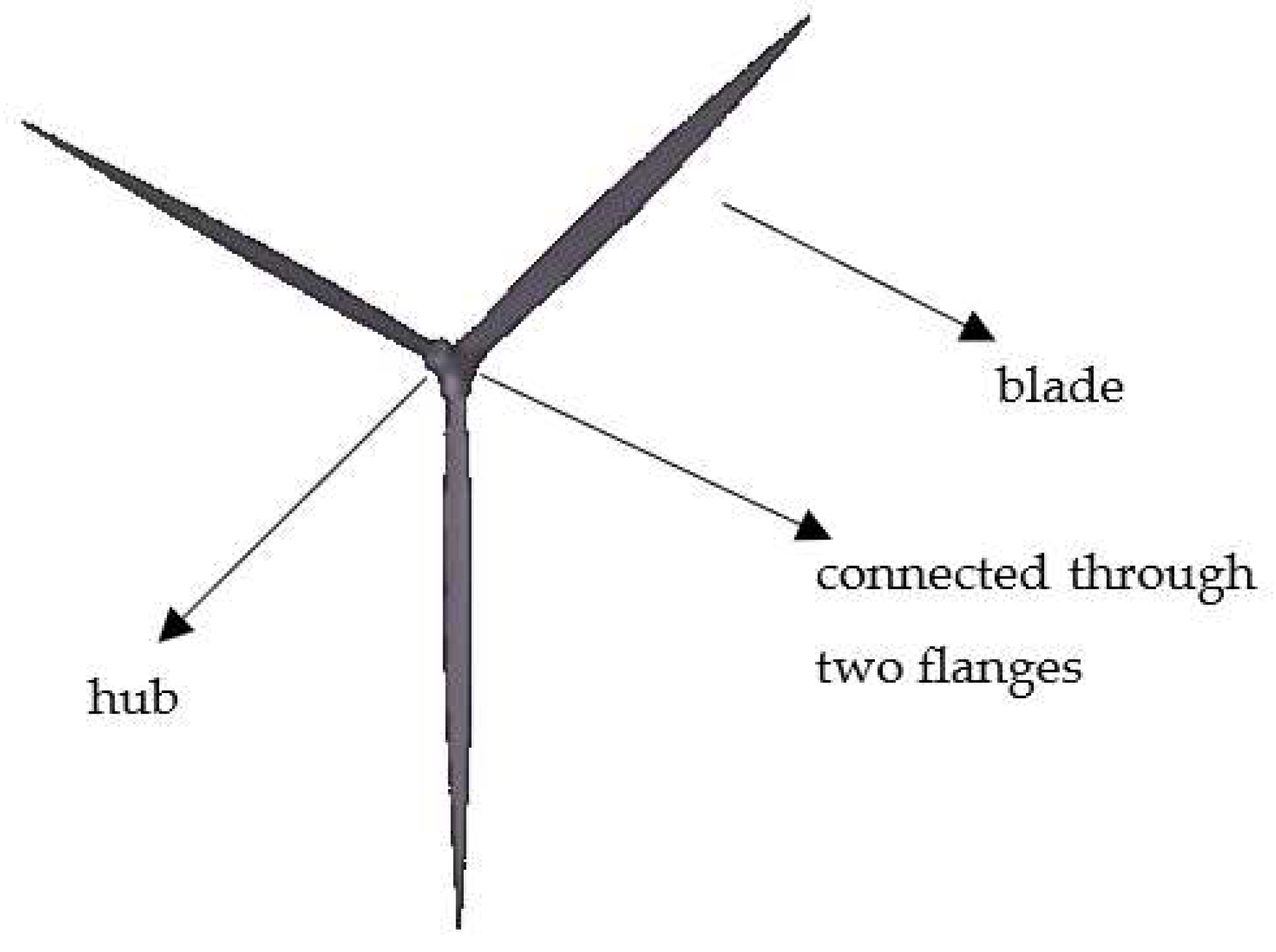
2.1.1. Wind Loads on the Impeller of Wind Turbine

The numerical method of wind load on the impeller of a wind turbine is introduced by discretizing the blade of the impeller into a finite number of smaller segments. According to the relationship between the drag coefficient C_d and lift coefficient C_l of the airfoil and the wind attack angle, the wind loads on each differential segment are calculated, respectively, which are as follows:

$$D={\displaystyle \frac{1}{2}}\rho c{v}_{rel}^2{C}_d$$

(1)

$$L={\displaystyle \frac{1}{2}}\rho c{v}_{rel}^2{C}_l$$

(2)

Usually, there is a certain twist angle between the airfoil section and the horizontal plane. So the lift and drag on the segment need to be decomposed into the normal and tangential directions of the impeller plane:

$$f_x=L\cos \alpha +D\sin \alpha$$

(3)

$$f_Z=L\sin \alpha +D\cos \alpha$$

(4)

The wind load on the blade can be obtained by integrating along the length direction of the blade. The impeller is composed of one hub and three blades. During the lifting process of the impeller, the impeller is presented as Y-shaped while one blade is vertical and the other two blades have a 30-degree angle with the horizontal plane, as shown in Figure 2. In this case, the wind load on the entire impeller is as follows:

$$\left[\begin{array}{l}{F}_x\\ F_y\\ F_z\\ M_x\\ M_y\\ M_z\end{array}\right]=\left[\begin{array}{c}{\displaystyle {\int }_{l}3f_{x}dl}+F_x\prime \\ \cos {\displaystyle \frac{\pi }{6}}{\displaystyle {\int }_l{f}_{z1}dl}+\cos {\displaystyle \frac{\pi }{6}}{\displaystyle {\int }_l{f}_{z2}dl}+{\displaystyle {\int }_l{f}_{z3}dl}+F_y\prime \\ 0\\ 3{\displaystyle {\int }_l{f}_{z1}ldl}\\ \cos {\displaystyle \frac{\pi }{6}}{\displaystyle {\int }_l{f}_{z1}ldl}+\cos {\displaystyle \frac{\pi }{6}}{\displaystyle {\int }_l{f}_{z2}ldl}+{\displaystyle {\int }_l{f}_{z3}ldl}\\ \cos {\displaystyle \frac{\pi }{6}}{\displaystyle {\int }_l{f}_{x1}ldl}+\cos {\displaystyle \frac{\pi }{6}}{\displaystyle {\int }_l{f}_{x2}ldl}\end{array}\right]$$

(5)

where $F_x\prime$ and $F_y\prime$ are the components of the wind load on the hub in the X-axis and Y-axis directions.

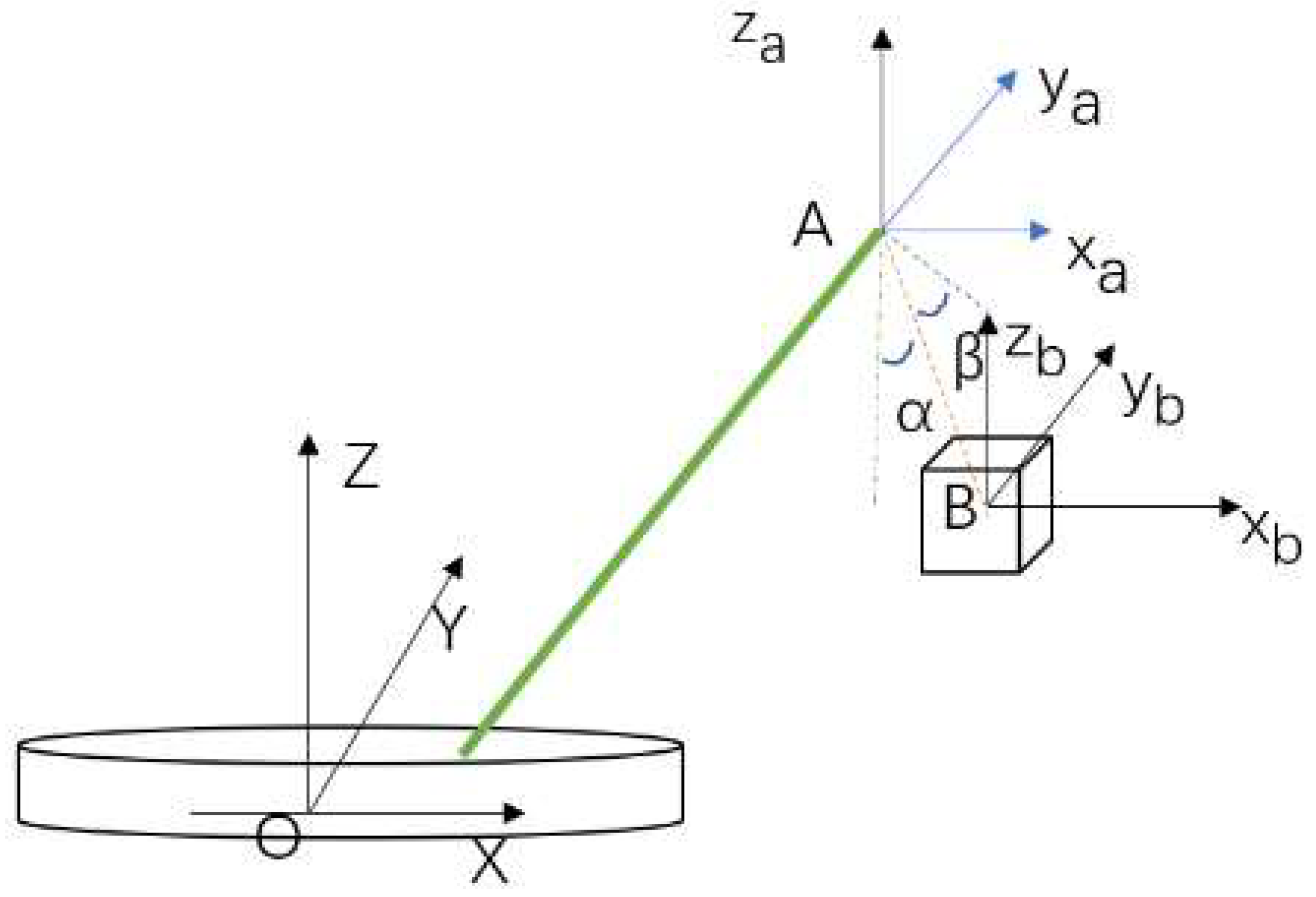
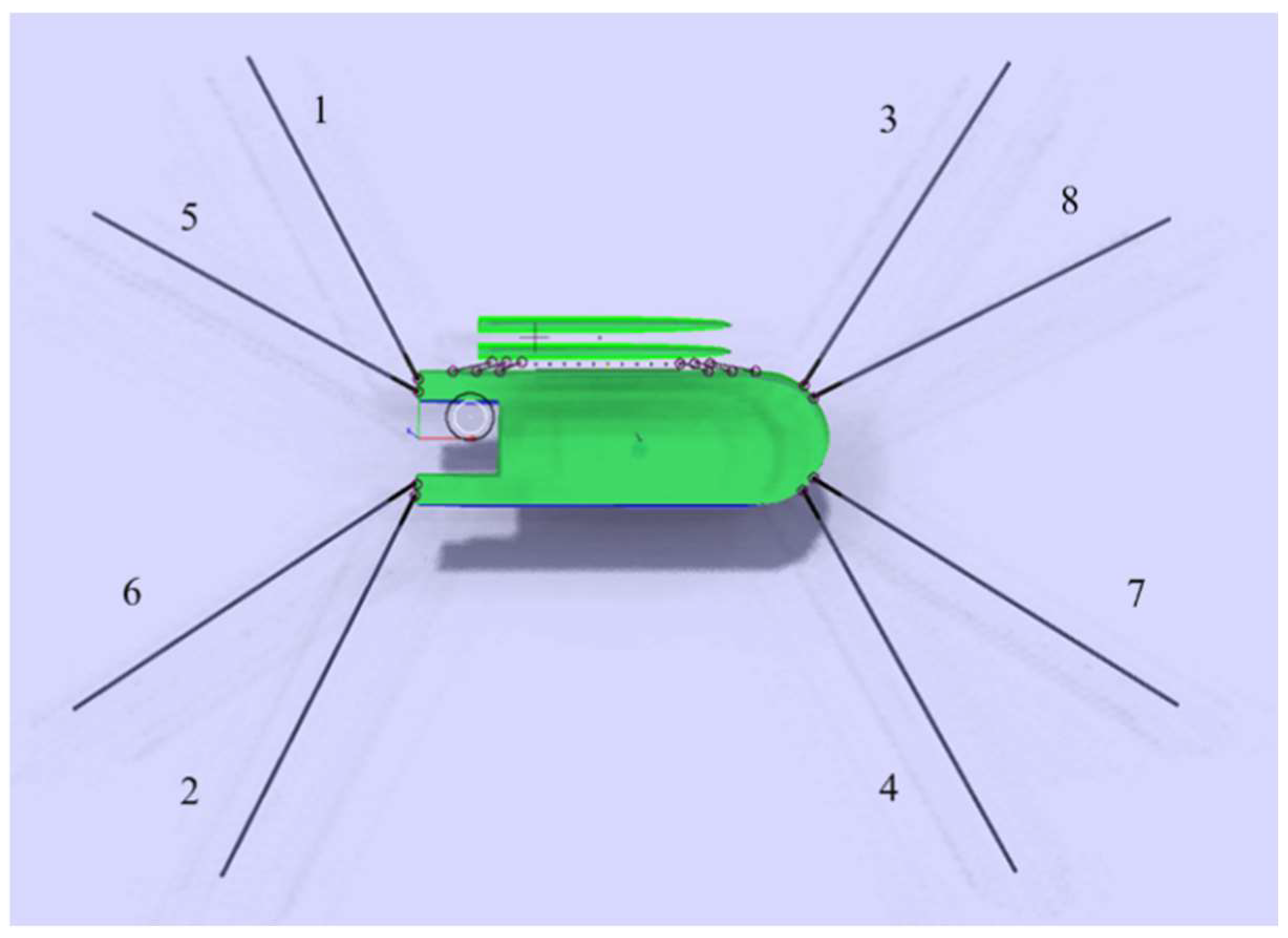
2.1.2. Hydrodynamics of Multi-Body (Two Floating Bodies)

There are motions of two adjacent floating bodies under the wave. In order to describe the movement of the floating body, three spatial coordinate systems are established. The origin of the global coordinate system O–XYZ, is set on the free horizontal plane without disturbance. Two local coordinate systems O₁–X₁Y₁Z₁ and O₂–X₂Y₂Z₂ are defined with the origins O₁ and O₂ in the center of gravity of the two floating bodies, respectively, as shown in Figure 3.

In the two adjacent floating bodies’ system, composed of floating body a with floating body b, the total radiation potential around the floating body a is the superposition of the radiation potential around floating body a caused by the motion of floating body a and b respectively. Coupled with the incident potential and the diffraction potential in the flow field, the total velocity potential of floating body a is obtained. The velocity potential ${\varphi }^{(a)}$, ${\varphi }^{(b)}$ of floating body a and floating body b can be expressed as follows:

$${\varphi }_a={\varphi }_I+{\varphi }_D+{\displaystyle \sum _{j=1}^6{\varphi }_j^{(aa)}i\omega }{\zeta }_j^{(a)}+{\displaystyle \sum _{j=1}^6{\varphi }_j^{(ba)}i\omega }{\zeta }_j^{(b)}$$

(6)

$${\varphi }_b={\varphi }_I+{\varphi }_D+{\displaystyle \sum _{j=1}^6{\varphi }_j^{(bb)}}i\omega {\zeta }_j^{(b)}+{\displaystyle \sum _{j=1}^6{\varphi }_j^{(ab)}i\omega }{\zeta }_j^{(a)}$$

(7)

where ${\varphi }_j^{(mn)}$ is the radiation velocity potential induced by the unit amplitude motion of the j-th degree of freedom of floating body m (m = a, b) around floating body n (n = a, b), ${\varphi }_j^{(ba)}$ is the radiation velocity potential generated by the unit amplitude motion of the j-th degree of freedom of the floating body b around floating body a, and ${\zeta }_j^{(m)}$ represents the motion amplitude of the j-th (j = 1, 2, …, 6) mode motion of floating body m (m = a, b).

The incident velocity potential ${\varphi }_I$ can be given directly as follows:

$${\varphi }_I={\displaystyle \frac{Ag\cosh k(z+h)}{\omega \cosh (kh)}}\exp [ik(x\cos \beta +y\sin \beta )]$$

(8)

where A is the wave amplitude, g is the acceleration of gravity, h is the water depth, k is the wave number, ω is the circular frequency of the wave, and β is the angle between the incident wave and the positive direction of the x-axis.

The governing equations and boundary conditions of the diffraction potential ϕ_D are given as follows:

$$\left\{\begin{array}{l}{\nabla }^2{\varphi }_D(x,y,z)=0\\ -{\omega }^2{\varphi }_D+{\displaystyle \frac{\partial {\varphi }_D}{\partial z}}=0,\left(z=0\right)\\ {\left.{\displaystyle \frac{\partial {\varphi }_D}{\partial n}}\right|}_{S_a}={\left.{\displaystyle \frac{\partial {\varphi }_I}{\partial n}}\right|}_{S_a},{\left.{\displaystyle \frac{\partial {\varphi }_D}{\partial n}}\right|}_{S_b}={\left.{\displaystyle \frac{\partial {\varphi }_I}{\partial n}}\right|}_{S_b}\\ {\left.{\displaystyle \frac{\partial {\varphi }_D}{\partial z}}\right|}_{Z=-H}=0\end{array}\right.$$

(9)

where S_a and S_b are the surfaces of floating bodies a and b and n is the normal vector on the surface of the floating body.

The solution of the radiation potential can be divided into two cases:

(1)

Floating body a is free, and floating body b is fixed;

(2)

Floating body a is fixed, and floating body b is free.

In case (1), the radiation velocity potentials around floating body a and floating body b are obtained, respectively.

$${\varphi }_R^{(a)}={\displaystyle \sum _{j=1}^6{\varphi }_j^{(aa)}i\omega }{\zeta }_j^{(a)}$$

(10)

$${\varphi }_R^{(b)}={\displaystyle \sum _{j=1}^6{\varphi }_j^{(ab)}i\omega }{\zeta }_j^{(a)}$$

(11)

For the radiation velocity potential ${\varphi }_R$, decomposed into the components ${\varphi }_j$ (j = 1, 2, …, 6) on the six motion modes, and the governing equations and boundary conditions, are given as follows:

$$\left\{\begin{array}{l}{\nabla }^2{\varphi }_j^{(an)}(x,y,z)=0\\ -{\omega }^2{\varphi }_j^{an}+{\displaystyle \frac{\partial {\varphi }_j^{an}}{\partial z}}=0,\left(z=0\right)\\ {\left.{\displaystyle \frac{\partial {\varphi }_j^{an}}{\partial n}}\right|}_{S_a}=n_j^{an}\\ {\left.{\displaystyle \frac{\partial {\varphi }_j^{an}}{\partial n}}\right|}_{S_b}=0\\ {\left.{\displaystyle \frac{\partial {\varphi }_j^{an}}{\partial z}}\right|}_{Z=-H}=0\\ \underset{R\to \infty }{\lim }\sqrt{R}({\displaystyle \frac{\partial {\varphi }_j^{an}}{\partial R}}-ik{\varphi }_j^{an})=0,\left(R=\sqrt{x^2+y^2+z^2}\right)\end{array}\right.$$

(12)

The governing equations and boundary conditions for case (2) can be obtained using the same method.

2.1.3. Lifting

The motion coupling model of the floating derrick–impeller is established, as shown in Figure 4. The coordinate system of the floating derrick is set with the origin point O in the center of gravity of the floating derrick. Point A is the lifting position of the crane, and point B is the center of gravity of the lifting object. The angle between the rope and the vertical direction of the lifting object is the swing angle of the lifting object.

Assuming the initial coordinate of point A is ($x_{a0},y_{a0},z_{a0}$), the motion equation of the lifting position A can be obtained:

$$\left[\begin{array}{c}{x}_a\\ y_a\\ z_a\end{array}\right]=\left[\begin{array}{cccccc}1& 0& 0& 0& z_{a0}& -y_{a0}\\ 0& 1& 0& -z_{a0}& 0& x_{a0}\\ 0& 0& 1& y_{a0}& -x_{a0}& 0\end{array}\right]{x_{oi}}^T\left(i=\mathrm{1,2}\dots 6\right)$$

(13)

where x_oi is the six-degree-of-freedom motion vector of the center of gravity of the floating derrick. Assuming the length of sling L, the coordinates of point B of the sling can be expressed as:

$$\left[\begin{array}{c}{x}_b\\ y_b\\ z_b\end{array}\right]=\left[\begin{array}{c}{x}_b\\ y_b\\ z_b\end{array}\right]+L\left[\begin{array}{c}\sin \alpha \cos \beta \\ \sin \beta \cos \alpha \\ \cos \alpha \end{array}\right]$$

(14)

The sling length L is regarded as an invariant constant, and the two angles are defined as variables. The equations of motion of the lifting object can be expressed as follows:

$$\left\{\begin{array}{l}\stackrel{..}{\alpha }-\stackrel{.}{{\beta }^2}\sin \alpha \cos \alpha +{\displaystyle \frac{{\stackrel{..}{x}}_a}{L}}\cos \alpha \sin \beta -{\displaystyle \frac{{\stackrel{..}{y}}_a}{L}}\cos \alpha \sin \beta +{\displaystyle \frac{{\stackrel{..}{z}}_a}{L}}\sin \alpha +{\displaystyle \frac{\mathrm{g}}{L}}\sin \alpha =0\\ \stackrel{..}{\beta }\sin \alpha +2 \stackrel{.}{\beta }\stackrel{.}{\alpha }\cos \alpha -{\displaystyle \frac{{\stackrel{..}{x}}_a}{L}}\sin \beta -{\displaystyle \frac{{\stackrel{..}{y}}_a}{L}}\cos \beta =0\end{array}\right.$$

(15)

Assuming the weight of the lifting objective M_B, it can be obtained from the motion mechanics:

$$M_B=\left[\begin{array}{c}{\stackrel{..}{x}}_b\\ {\stackrel{..}{y}}_b\\ {\stackrel{..}{z}}_b\end{array}\right]+T\left[\begin{array}{c}\sin \alpha \cos \beta \\ \sin \beta \cos \alpha \\ \cos \alpha \end{array}\right]$$

(16)

where T is the sling tension.

The dynamic tension of the sling is obtained:

$$\left\{\begin{array}{c}T=M_{B}g\cos \alpha +M_{B}L\left[{\stackrel{.}{\alpha }}^2+{\stackrel{.}{\beta }}^2{\sin }^2\alpha -f\right]\\ f=M_B\left({\stackrel{..}{x}}_b\sin \alpha \cos \beta -{\stackrel{..}{y}}_b\sin \alpha \sin \beta -{\stackrel{..}{z}}_b\cos \beta \right)\end{array}\right.$$

(17)

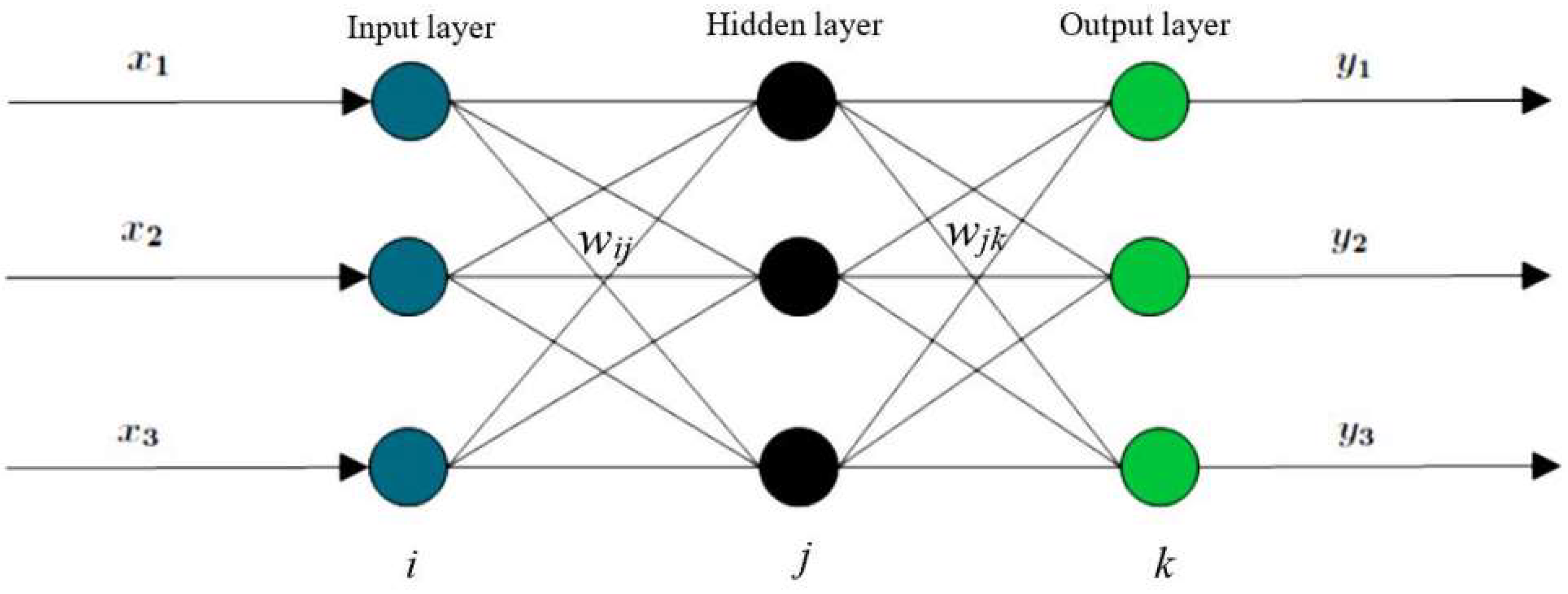
2.2. BP Neural Network Theory

In a BP neural network, there are m nodes in an input layer, q nodes in the hidden layer, and ri nodes in the output layer. The weight of the network remains unchanged during the forward propagation of input signal Xi. After the processing of the hidden layer, the actual output Y is obtained in the output layer, and the error between Y and the expected output Y~ is calculated by the error function. If the error is too large, it is transferred to the reverse broadcast process.

F(x) is the hidden layer activation function. Taking the Sigmoid function as an example, the process of forward propagation of the neural network is as follows:

$$F\left(x\right)={\displaystyle \frac{1}{1+e^{-ax}}}$$

(18)

The input value of the j-th node of the hidden layer h_j can be obtained:

$$h_j=\sum _{i=1}^m\left(w_{ij}{x}_i-{\gamma }_j\right)$$

(19)

where w_ij is the connection weight of the i-th node of the input layer and the j-th node of the hidden layer, and γ_j is the threshold of the j-th node of the hidden layer.

The output value of the j-th node in the hidden layer H_j is obtained:

$$H_j=F\left(h_j\right)$$

(20)

The actual output value of the k-th node in the output layer Y_k can be obtained:

$$Y_k=\sum _{k=1}^n{H}_j{w}_{jk}-{\theta }_k,\hspace{1em}k=\mathrm{1,2}\dots n$$

(21)

where w_jk is the connection weight between the j-th node of the hidden layer and the k-th node of the output layer, and θ_k is the threshold of the k-th node in the output layer.

Error Back Propagation Process

The error signal starts to propagate forward from the output layer in some way. The weights and thresholds of the network will be adjusted continuously with the feedback of the error signal until the actual output and the expected output are kept within the acceptable error range. This is the reverse working process of the BP neural network.

Assuming that the number of samples is C, and the expected output of the p-th sample at the k-th node is $T_k^p$, then the error of the C sample data can be obtained according to the error criterion function:

$$e_k={\displaystyle \frac{1}{2}}{\sum _{P=1}^C\sum _{k=1}^n\left(T_k^p-Y_k^p\right)}^2{e}_k$$

(22)

According to the BP neural network, the gradient descent method is used to correct:

$$\begin{gathered} \Delta w_{ij}=-\eta {\displaystyle \frac{\partial e}{\partial w_{ij}}} \\ \Delta {\gamma }_j=-\eta {\displaystyle \frac{\partial e}{\partial {\gamma }_j}} \\ \Delta w_{jk}=-\eta {\displaystyle \frac{\partial e}{\partial w_{jk}}} \\ \Delta {\theta }_k=-\eta {\displaystyle \frac{\partial e}{\partial {\theta }_k}} \end{gathered}$$

(23)

The above several simultaneous solutions can be used to obtain the weight variation of the hidden layer of the network:

$$\Delta w_{ij}=-\eta {\displaystyle \frac{\partial e}{\partial w_{ij}}}=-\eta {\displaystyle \frac{\partial e}{\partial h_j}}{\displaystyle \frac{\partial h_j}{\partial w_{ij}}}=-\eta {\displaystyle \frac{\partial e}{\partial h_j}}{\displaystyle \frac{\partial h_j}{\partial Y_k}}{\displaystyle \frac{\partial Y_k}{\partial w_{ij}}}$$

(24)

The threshold change in the network hidden layer is:

$$\Delta {\gamma }_j=-\eta {\displaystyle \frac{\partial e}{\partial {\gamma }_j}}=-\eta {\displaystyle \frac{\partial e}{\partial h_j}}{\displaystyle \frac{\partial h_j}{\partial {\gamma }_j}}=-\eta {\displaystyle \frac{\partial e}{\partial h_j}}{\displaystyle \frac{\partial h_j}{\partial Y_k}}{\displaystyle \frac{\partial Y_k}{\partial {\gamma }_j}}$$

(25)

The network output layer connection weight variation is:

$$\Delta w_{jk}=-\eta {\displaystyle \frac{\partial e}{\partial w_{jk}}}=-\eta {\displaystyle \frac{\partial e}{\partial h_j}}{\displaystyle \frac{\partial h_j}{\partial w_{jk}}}=-\eta {\displaystyle \frac{\partial e}{\partial h_j}}{\displaystyle \frac{\partial h_j}{\partial Y_k}}{\displaystyle \frac{\partial Y_k}{\partial w_{jk}}}$$

(26)

The variation of the network output connection threshold is:

$$\Delta {\theta }_k=-\eta {\displaystyle \frac{\partial e}{\partial {\theta }_k}}=-\eta {\displaystyle \frac{\partial e}{\partial h_j}}{\displaystyle \frac{\partial h_j}{\partial {\theta }_k}}=-\eta {\displaystyle \frac{\partial e}{\partial h_j}}{\displaystyle \frac{\partial h_j}{\partial Y_k}}{\displaystyle \frac{\partial Y_k}{\partial {\theta }_k}}$$

(27)

And because:

$$\begin{gathered} \eta {\displaystyle \frac{\partial e}{\partial h_j}}=-\sum _{p=1}^C\sum _{k=1}^n\left(T_k^p-Y_k^p\right)\hspace{1em}\hspace{1em}\hspace{1em}\hspace{1em} \\ {\displaystyle \frac{\partial h_j}{\partial w_{ij}}}=y_i;{\displaystyle \frac{\partial h_j}{\partial {\gamma }_j}}=1;{\displaystyle \frac{\partial h_j}{\partial w_{jk}}}=x_k;{\displaystyle \frac{\partial h_j}{\partial {\theta }_k}}=1; \end{gathered}$$

(28)

$$\eta {\displaystyle \frac{\partial e}{\partial y_j}}=-\sum _{p=1}^C\sum _{k=1}^n\left(T_k^p-Y_k^p\right)h_j{w}_{ij}$$

(29)

$${\displaystyle \frac{\partial y_j}{\partial h_j}}=h_j$$

(30)

$${\displaystyle \frac{\partial Y_k}{\partial H_k}}=H_k$$

(31)

The final adjustment of the weight threshold of each layer of the BP neural network is as follows:

$$\Delta w_{ij}=\eta \sum _{p=1}^C\sum _{k=1}^n\left(T_k^p-Y_k^p\right)H_k{w}_{jk}{h}_j{x}_k$$

(32)

$$\Delta {\gamma }_j=\eta \sum _{p=1}^C\sum _{k=1}^n\left(T_k^p-Y_k^p\right)h_j$$

(33)

$$\Delta w_{jk}=\eta \sum _{p=1}^C\sum _{k=1}^n\left(T_k^p-Y_k^p\right)h_j{y}_j$$

(34)

$$\Delta {\theta }_k=\eta \sum _{p=1}^C\sum _{k=1}^n\left(T_k^p-Y_k^p\right)H_k{w}_{jk}{h}_j$$

(35)

The structure diagram of the BP neural network is as follows.

In Figure 5, X_n is the input variable; i, j, and k are the number of nodes in the input layer, the hidden layer, and the output layer respectively; w_ij and w_jk are the connection weights between the layers, respectively; and y_ij and y_jk are the output value of the hidden layer and the output value of the output layer, respectively.

2.3. Numerical Model and Validation

2.3.1. Numerical Model

In the process of offshore wind turbine installation, the floating derrick is usually working in cooperation with a deck cargo ship in China to improve efficiency. In this paper, the parameters of the floating derrick and the catamaran deck cargo ship are listed in

Table 1. Main parameters of the working ships.

Items	Variable	Unit	Ship Type
			Floating Derrick	Deck Cargo Ship
Length	$L_{oa}$	m	143	88
Waterline length	$L_{WL}$	m	141	86
Length between perpendiculars	$L_{BP}$	m	137	82
Width	B	m	46.4	15
Width of one sheet	b	m	-	5.6
Depth	D	m	10.8	4
Draft	d	m	7.5	3
Displacement	$\Delta$	t	40,682	1064
Vertical position of center of gravity	KG	m	3.62	5.12
Longitudinal position of center of gravity	LCG	m	76.13	42.2
Inertia radius of roll	$K_{xx}$	m	13.48	5.31
Inertia radius of pitch	$K_{yy}$	m	33.20	25.94
Inertia radius of yaw	$K_{zz}$	m	35.82	26.2

.

In order to ensure the stability, safety, and efficiency of the floating derrick, the ship is positioned by eight moorings named 1 to 8, with 400 m lengths per line, as shown in Figure 6. The deck cargo ship is positioned using a side-by-side system, which consists of fenders and cables that connect it to the floating derrick. The operating water depth is 50 m. The specific arrangement scheme and materials of the mooring lines are listed in

Table 2. Parameters of mooring line arrangement.

Mooring Line Number	Pretension (kN)	Azimuth (deg)	Fairlead
			X	Y	Z
1	1100	120	−76	20.05	3.3
2	1100	−120	−76	−20.05	3.3
3	1100	60	56.5	18	3.3
4	1100	−60	56.5	−18	3.3
5	1100	150	−76	15.85	3.3
6	1100	−150	−76	−15.85	3.3
7	1100	30	60	14	3.3
8	1100	−30	60	−14	3.3

and

Table 3. Material parameters of mooring lines.

Diameter m	Dry Weight kg/m	Wet Weight kg/m	Stiffness kN	Broken Strength kN
0.076	123	98.4	6.75 × 106	8520

.

The lifting process of the impeller is investigated in this paper. Since the lifting of the floating derrick is a complex multi-body system, the following assumptions are applied:

(1)

The crane on the floating derrick is a rigid body as a whole, ignoring the deformation during its operation;

(2)

Compared with the large mass of the impeller, the mass of the sling is ignored in the numerical simulation.

Based on the above hypothesis, the floating derrick–impeller coupling model is established, as shown in Figure 7. The impeller model used is based on the 5 MW offshore wind turbine model published by the NREL [26]. The blade of the wind turbine with the parameters in

Table 4. Parameters of wind turbine impeller.

Items	Unit	Value
Number of blades	-	3
Blade length	m	61.5
Impeller diameter	m	126
Hub diameter	m	3
Hub mass	Kg	56,780
Leaf mass	Kg	17,740

is composed of six airfoils with a total of 17 sections, and the root of the blade is connected to the hub through two cylinders, as shown in Figure 2.

During the lifting operation of the floating derrick, the motion of the ship, including roll, pitch, and heave, has a serious impact on the stability of the operation. Under the coupling effect of the floating crane system and the impeller, the ship sloshing will also affect the motion of the impeller. Therefore, the roll, pitch, and heave of the floating derrick and the motion of the impeller, including sway, surge, and heave, are focused on in this paper.

2.3.2. Comparison Between Numerical and Experimental Results

The hydrodynamic analysis of the multi-floating body system is performed by SESAM/SIMA based on three-dimensional potential flow theory, as shown in Figure 8a, while the scaled experiment model of the double-floating body system is shown in Figure 8b. The main dimensions of the test models, with a scale of 1:80, are listed in

Table 5. Main dimensions of the test models.

Items		Unit	Barge 1		Barge 2
			Original Ship	Test Model	Original Ship	Test Model
Length	Loa	m	207	2.5875	235.6	2.9450
Length between perpendiculars	LBP	m	194	2.4250	225	2.8125
Breadth	B	m	36	0.4500	46	0.5750
Depth	D	m	16	0.2000	24.1	0.3013
Draft	d	m	8.7	0.1088	11	0.1375
Displacement	$\Delta$	t	49,444	0.0942	104,748.4	0.1996
Vertical position of center of gravity	KG	m	11.8	0.1475	10.242	0.1280
Center of gravity longitudinal position	LCG	m	1.8	0.0225	−2.0	−0.0250

, and the test conditions are shown in

Table 6. Test condition.

Irregular Wave	Unit	Actual Value	Test Value
Significant wave height	m	2.5	0.03
Spectral periods	s	10	1.1
Direction	deg	180°	180°

.

Through the calculation of the RAOs of the double-floating body system in the frequency domain, the hydrodynamic model in the time domain is established using the frequency and time domain transformation method. In the numerical analysis, the damping coefficients are input using the results obtained by the Stillwater decay experiment. Then, the six-degree-of-freedom motion response time history curve of the two barges is obtained under the environment condition in Table 6.

Through the irregular wave experiment, the motion response time history curve of the two barges can be obtained under the conditions in Table 6. The maximum and minimum values are illustrated in Figure 9 in the direction of surge, sway, heave, roll, pitch, and yaw. In Figure 9a,b, the max and min results are compared for Barge 1, as well as the errors for the six-degree motions. It can be seen that the numerical results are larger than the ones obtained by the experiments. It may induced by the simplification of the cables connecting the two ships, as the damping is not included in the numerical analysis comparing the experiments. The maximum error for Barge 1 occurs at the min results of the sway motion, 11.54%, while others are less than 10%, as shown in Figure 9c. Meanwhile, the maximum error for Barge 2 occurs at the max results of the yaw motion, 13.70%, while the others are less than 10%, as shown in Figure 9f. It can be seen that the numerical method is verified, as the error is small.

3. Hydrodynamics Parameters of the Floating Derrick and Cargo Ship

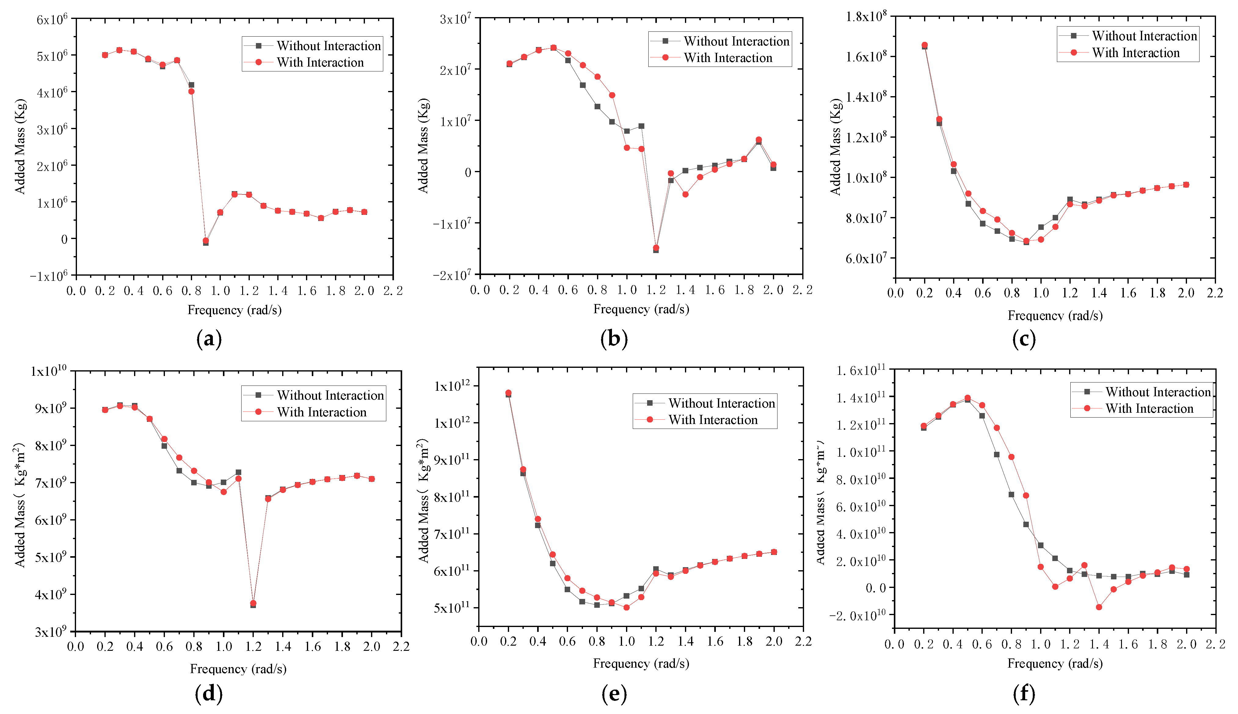
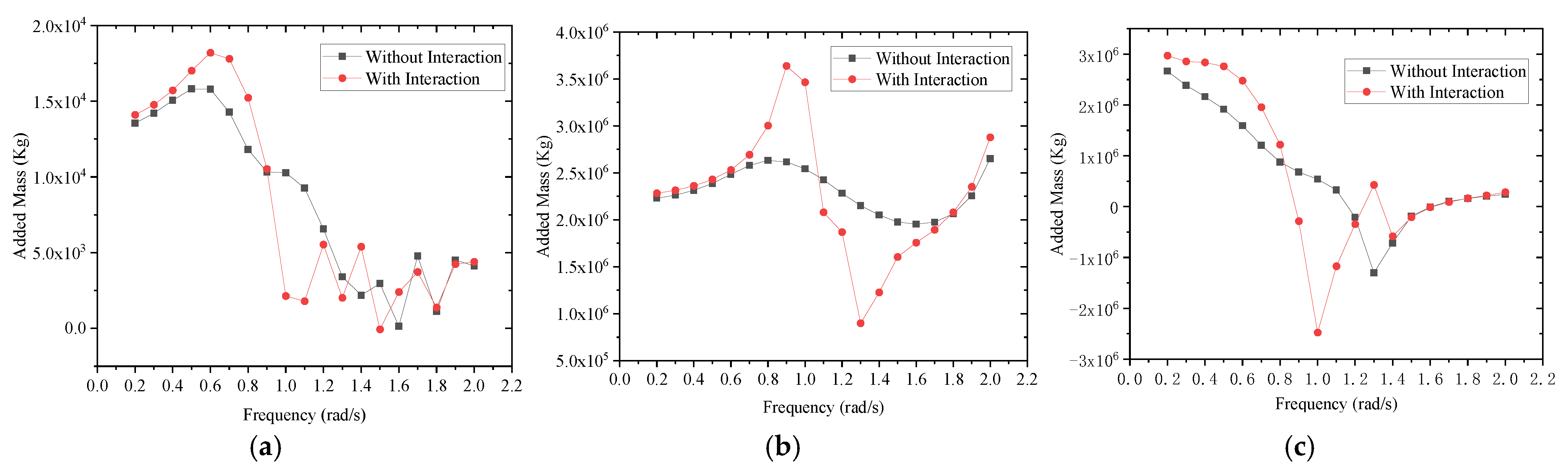
As shown in Figure 5, the floating derrick is working when coupled with the cargo ship, as the two floating bodies described in Section 2.1.2. The hydrodynamic parameters, such as added mass, radiation damping, response amplitude operator, and wave force, may be changed for the coupled model compared with the single one. The hydrodynamics parameters of the floating derrick and cargo ship are investigated.

3.1. Added Mass

The added mass of the floating derrick is shown in Figure 10, considering the interaction of the deck cargo ship, while the added mass of the cargo ship is shown in Figure 11. As the main dimension of the floating derrick is much larger than the cargo ship, the interaction of the two ships has little effect on the added mass of the floating derrick. As shown in Figure 10a, the added mass in the surge of the model, considering the interaction of the cargo ship, is almost the same as the results without the cargo ship. As the wave frequency is in the range of 0.6–1.6 rad/s, an obvious difference occurs in the added mass of sway and yaw, as shown in Figure 10b,f, but there is little difference between the low and high frequencies when comparing the results with and without the interaction of the two ships. Meanwhile, some difference occurs in the heave, roll, and pitch of the wave frequency 0.4–1.2 rad/s, in Figure 10c–e.

The floating derrick will induce a large influence on the added mass of the cargo ship. A large influence occurs with the added mass in the sway, heave, roll, pitch, and yaw in the wave frequency range of 0.6–1.4 rad/s. As shown in Figure 11a, the maximum difference of the added mass in surge occurs as the frequency is 1.1 rad/s. Meanwhile, the maximum difference in the added mass in sway occurs at the frequency of 1.3 rad/s, in Figure 11b; in heave at the frequency of 1.0 rad/s, in Figure 11c; in roll at the frequency of 1.3 rad/s, in Figure 11d; in pitch at the frequency of 1.0 rad/s, in Figure 11e; and in heave at the frequency of 1.3 rad/s, in Figure 11f.

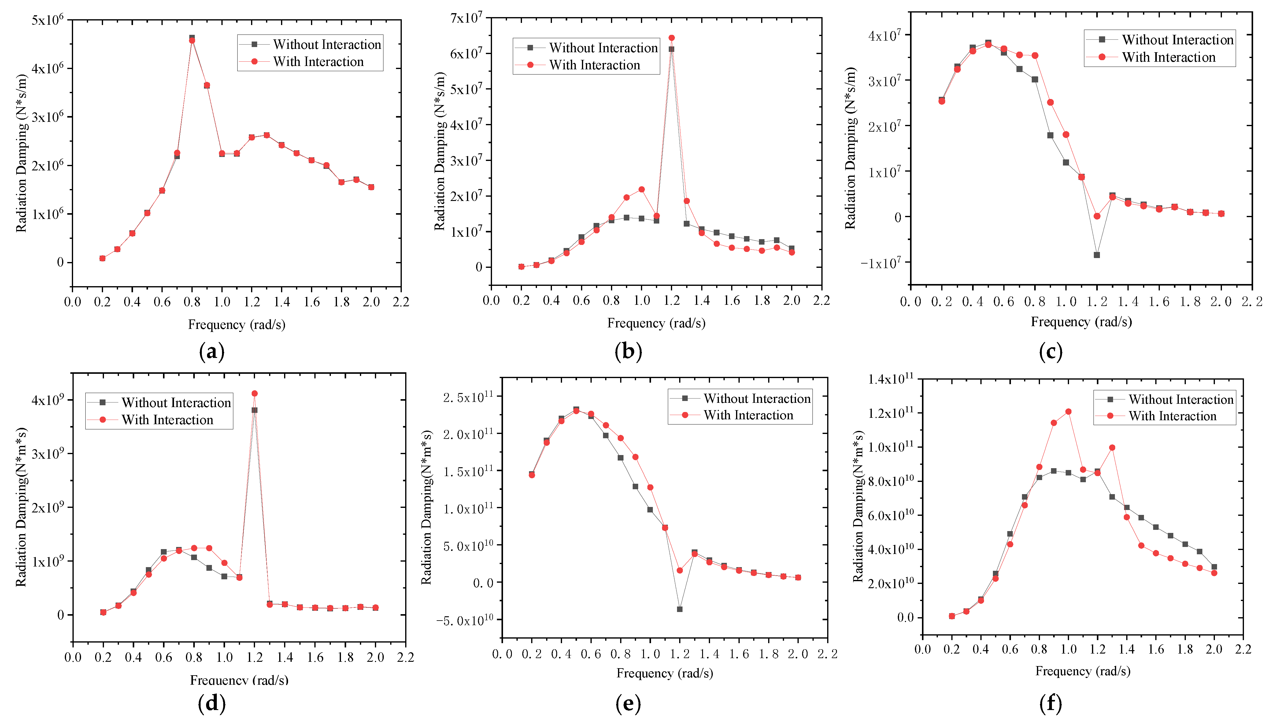
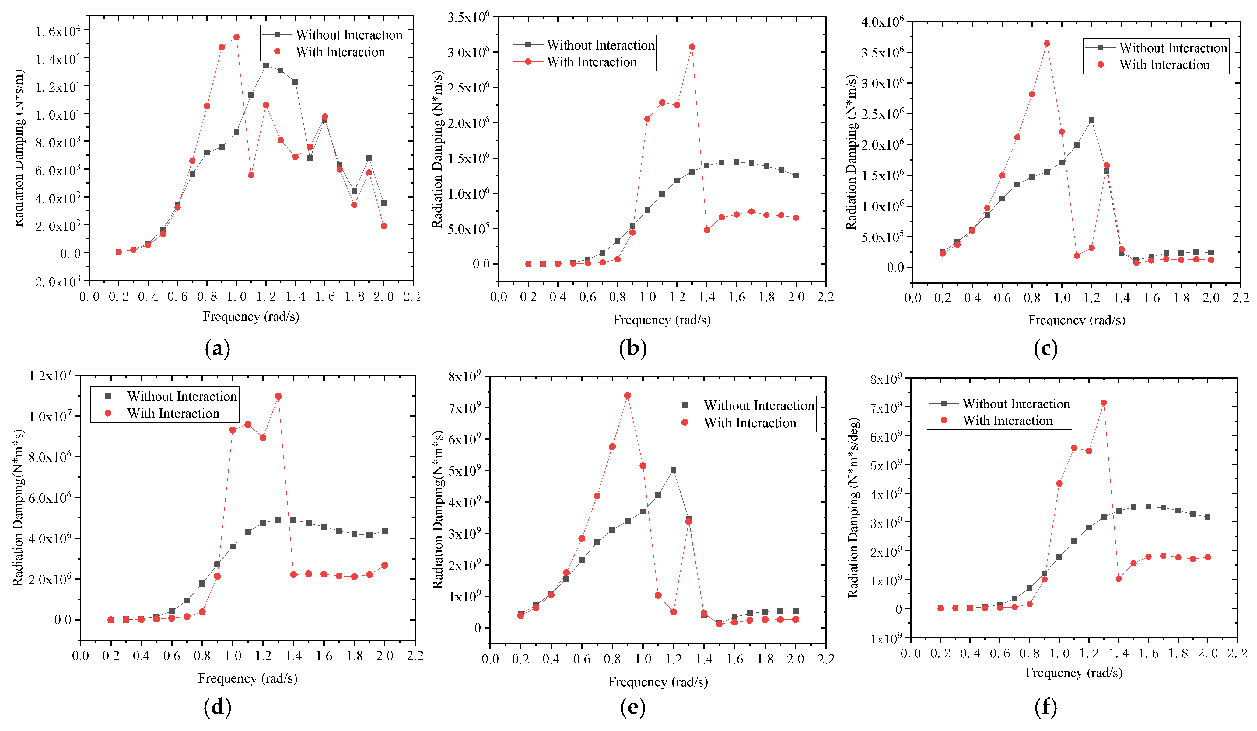
3.2. Radiation Damping

The radiation damping of the floating derrick and the cargo ship with and without interaction are shown in Figure 12 and Figure 13, respectively. The influence on the radiation damping of the floating derrick has the same trend as the added mass. Little difference occurs in the radiation in the surge of the floating derrick, as in Figure 12a. In the frequency range of 0.6–1.2 rad/s, some difference occurs in the radiation in the sway, heave, roll, and pitch of the floating derrick, as shown in Figure 12b–e. The obvious difference occurs in the radiation in the yaw, as the frequency is larger than 0.8 rad/s.

Meanwhile, due to the influence of the large floating derrick, the radiation damping of the cargo ship will change obviously, by comparing the results without interaction as the frequency is larger than 0.4 rad/s, in the surge direction in Figure 13a, in the sway in Figure 13b, in the heave in Figure 13c, in the roll in Figure 13d, in the pitch in Figure 13e, and in the yaw in Figure 13f.

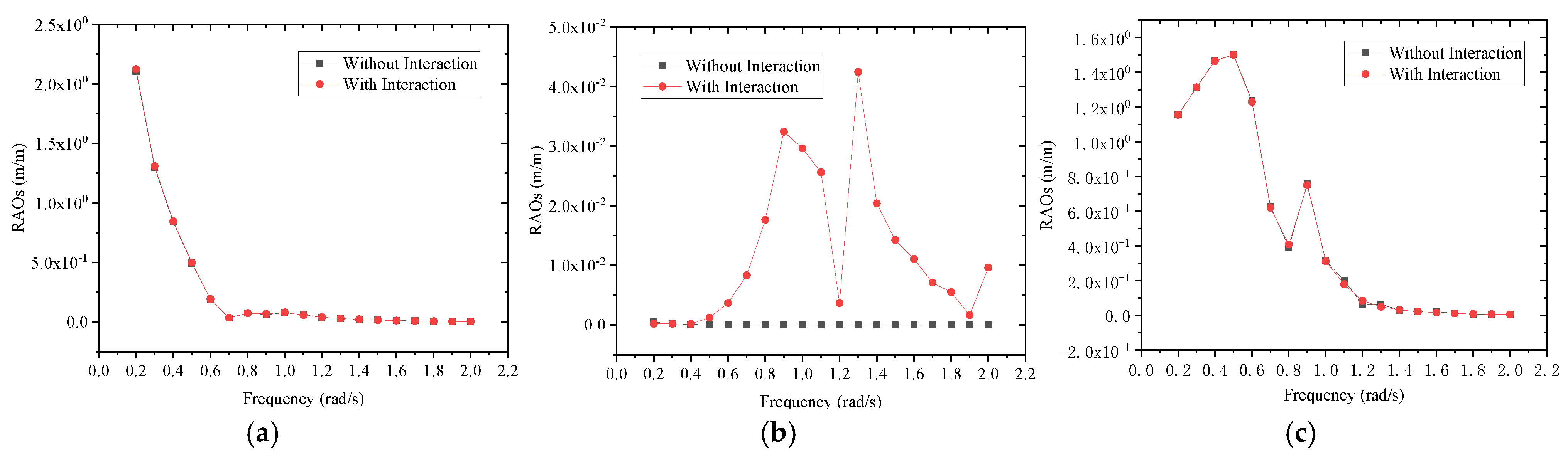
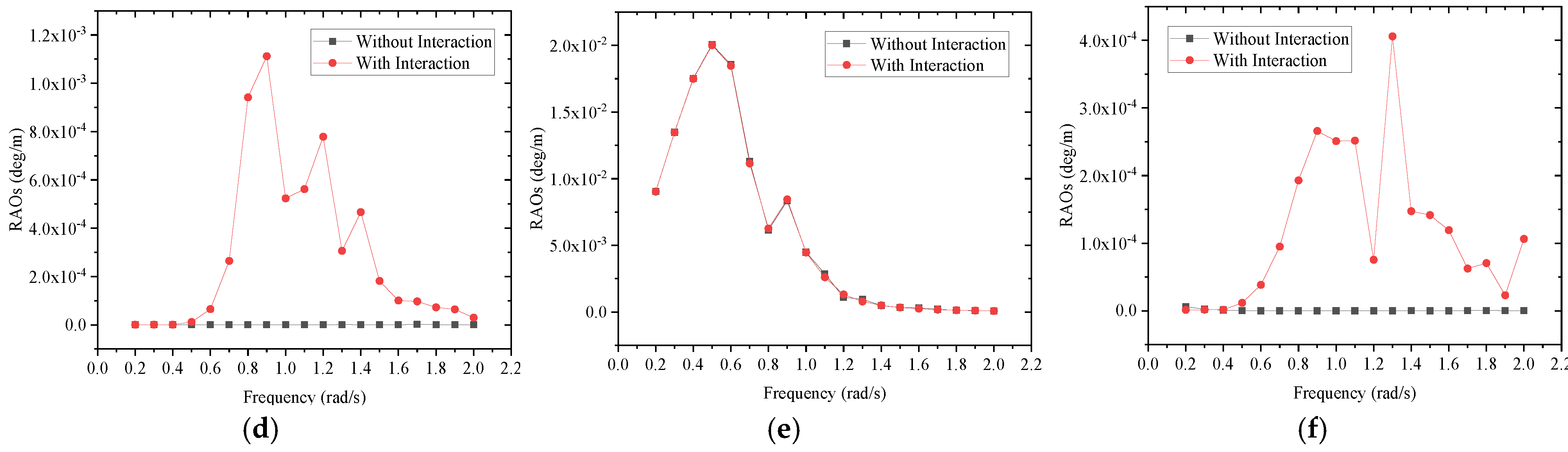
3.3. Response Amplitude Operator (RAO)

To reduce the influence of the environmental load, the floating derrick is usually set to face the wave, avoiding the beam wave. The RAOs in the direction of 180 degrees of the floating derrick and the cargo ship are investigated, as shown in Figure 14 and Figure 15, respectively.

In Figure 14, the multi-body effect on the RAO is significant on the RAOs of the floating derrick in sway, roll, and yaw, as shown in Figure 14b,d,f, and there is little effect on the other motions in Figure 14a,c,e, compared with the RAOs of the results without interaction.

Considering the effect of the floating derrick, the RAOs of the cargo ship are different from the ship only in sway, heave, roll, pitch, and yaw, as illustrated in Figure 15b–f, but there is little difference in surge in Figure 15a.

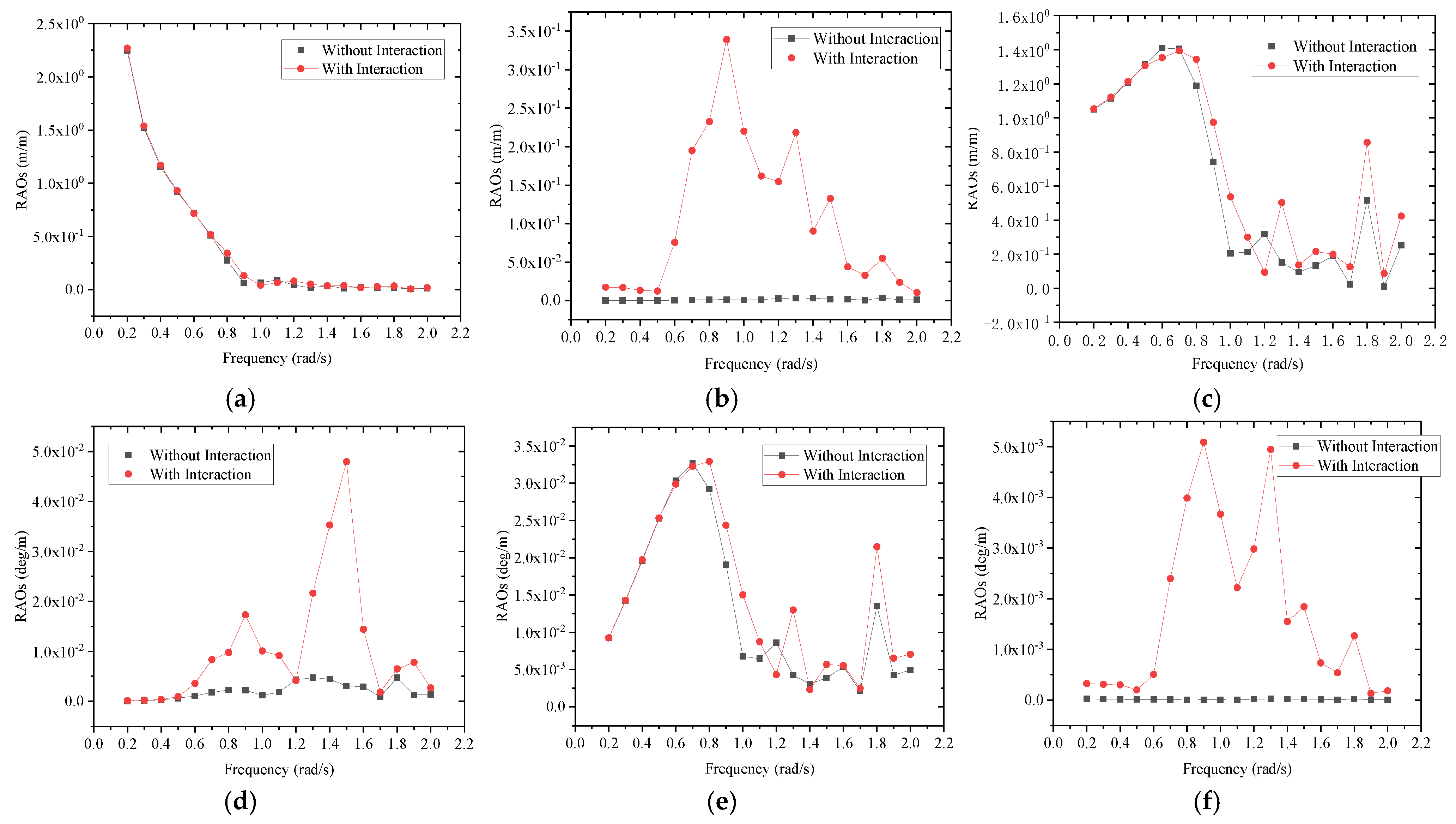
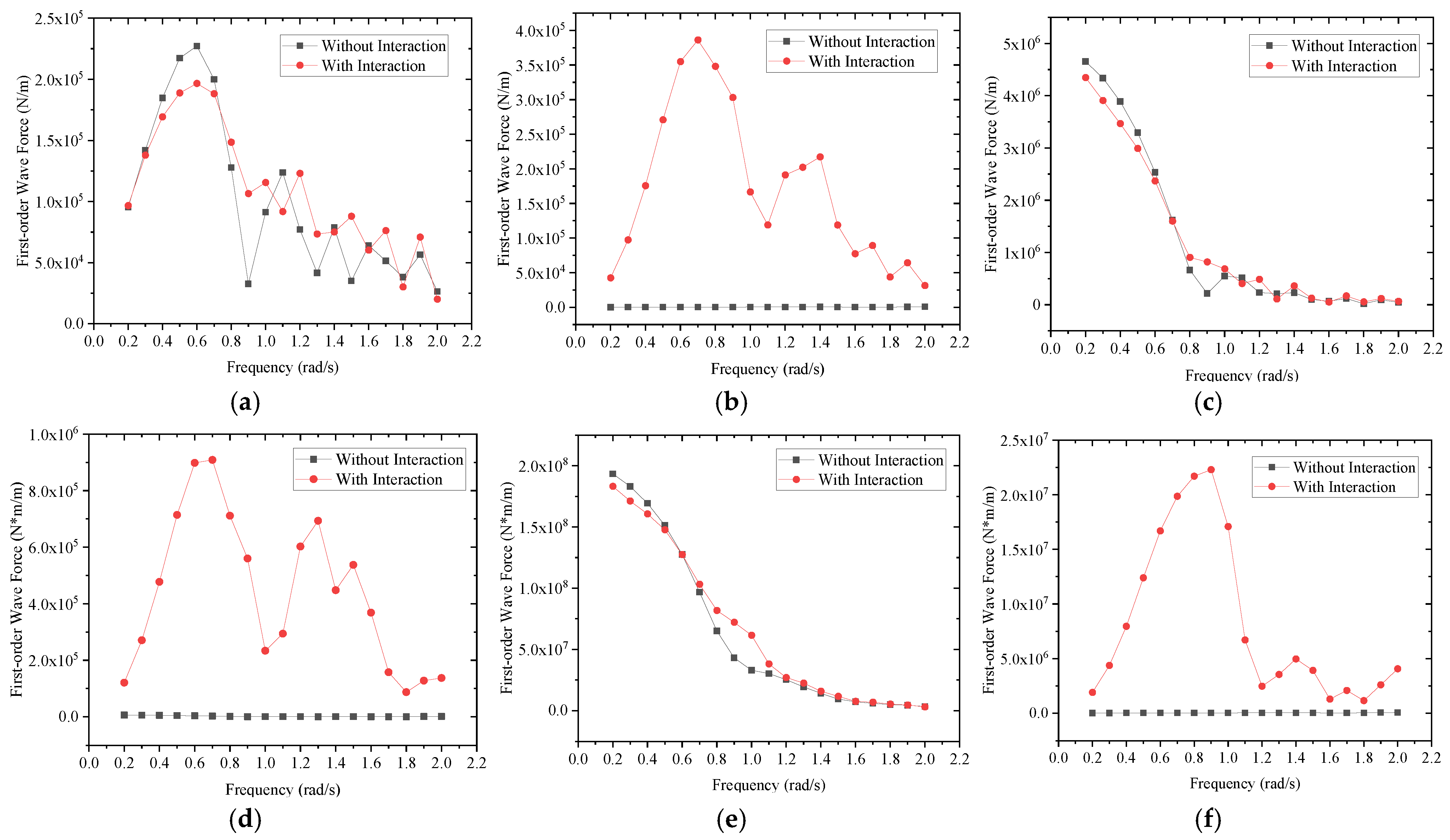
3.4. First-Order Wave Force

The first-order wave force in the direction of 180 degrees is calculated for the floating derrick and the cargo ship, including the interaction of the two ships. Comparing the results of the floating derrick in Figure 16, the cargo ship may have an obvious effect on the first-order wave force in sway, roll, and yaw, and enlarge the force. And the floating derrick may affect the first-order wave force of the cargo ship in all six-degree motions, as shown in Figure 17.

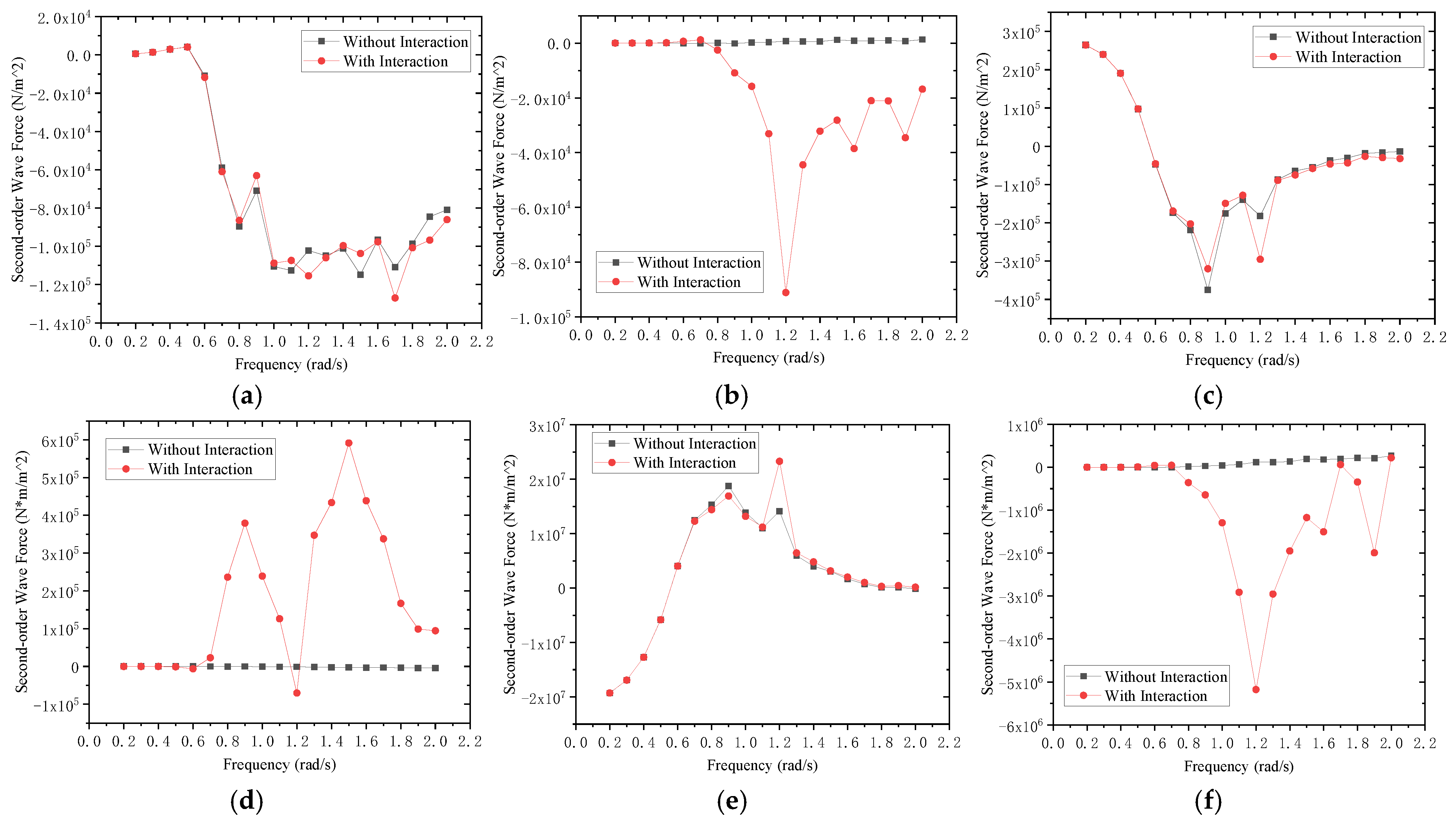
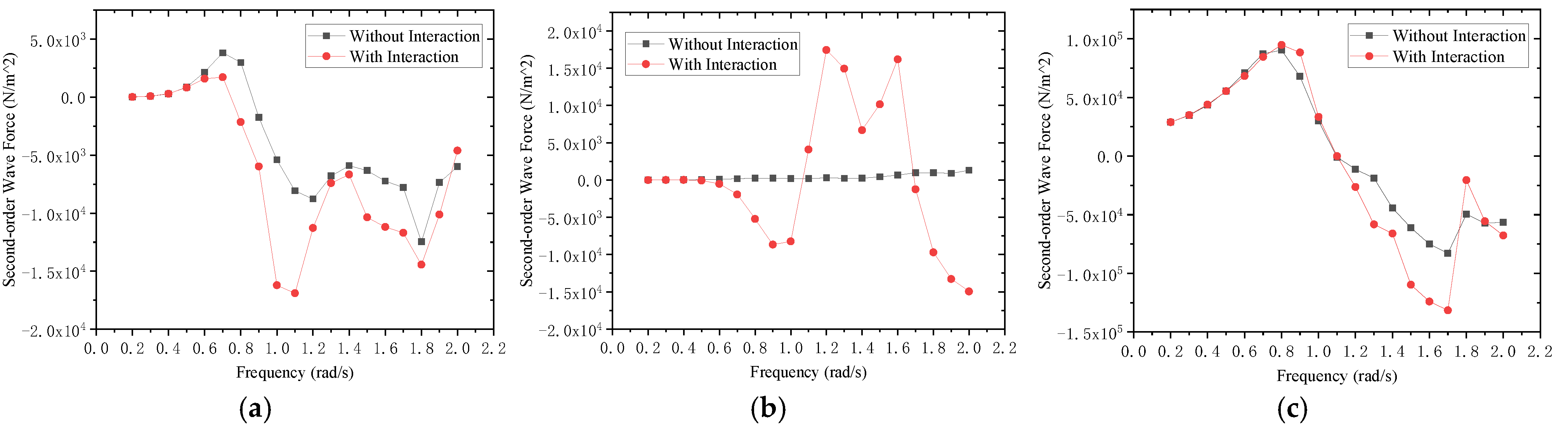
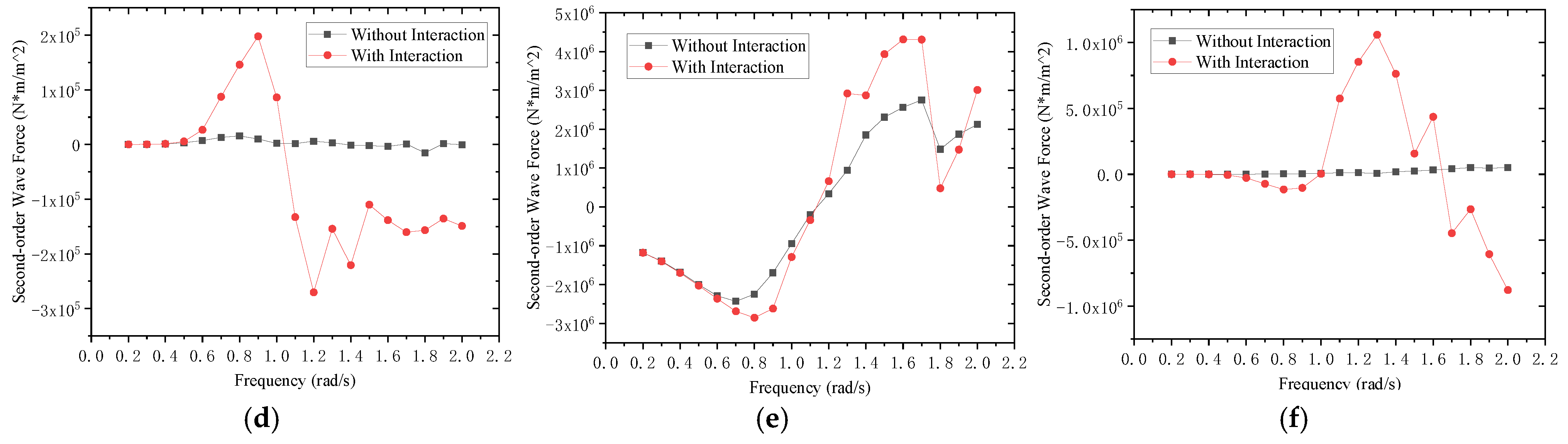
3.5. Second-Order Wave Force

Comparing the first-order wave force, the second-order force of the floating derrick and cargo ship is calculated as the velocity potential function is expanded by the second-order Taylor series by the QTF method. The results in the direction of 180 degrees are shown in Figure 18 and Figure 19 for the floating derrick and the cargo ship, respectively.

The interaction of the two ships may have a significant influence on the second-order wave force of the floating derrick, as the frequency is more than 0.8 rad/s, which enlarges the value but has little effect in low frequency, as in Figure 18. The same influence trend happens to the cargo ship, as shown in Figure 19.

4. Influencing Factors Analysis

In the lifting analysis model of the floating derrick, the wave, wind, and current will affect the motion of the ship, which will enlarge or reduce the motion of the lifting impeller. Meanwhile, the wind and lifting height will have an influence on the motion of the impeller, which will also affect the ship’s motions. The change in rotation angle will change the gravity of the floating system, inducing the motion change of the ship. All the factors are investigated to obtain the motions of the ship and lifting impeller.

4.1. Environmental and Lifting Parameters

In order to study the factors that affect the floating crane operation, the frequency distribution of the wave period and the significant wave height in the East China Sea [27] are chosen to investigate the operation probability of the floating derrick in objective sea areas, as shown in Figure 20. And the parameters are listed in

Table 7. Environmental parameters.

Items	Value
Wave spectrum	JONSWAP
Wind spectrum	NPD
Wind velocity m/s	3–9
Current velocity m/s	0.5–1.5
Significant wave height m	1.25–2.0

.

In order to reveal the influence of the lifting parameters, such as the lifting height and the boom rotation angle on the ship and the lifting object in the offshore wind turbine installation, a series of the lifting parameters are listed in

Table 8. Specific parameter values of simulation calculation.

Items	Value
Lifting height m	70/80/90
Hoisting arm elevation angle °	75
Crane rotation velocity m/s	0.2
The boom rotation angle °	0/45/90/135/180

.

4.2. Environmental Factors

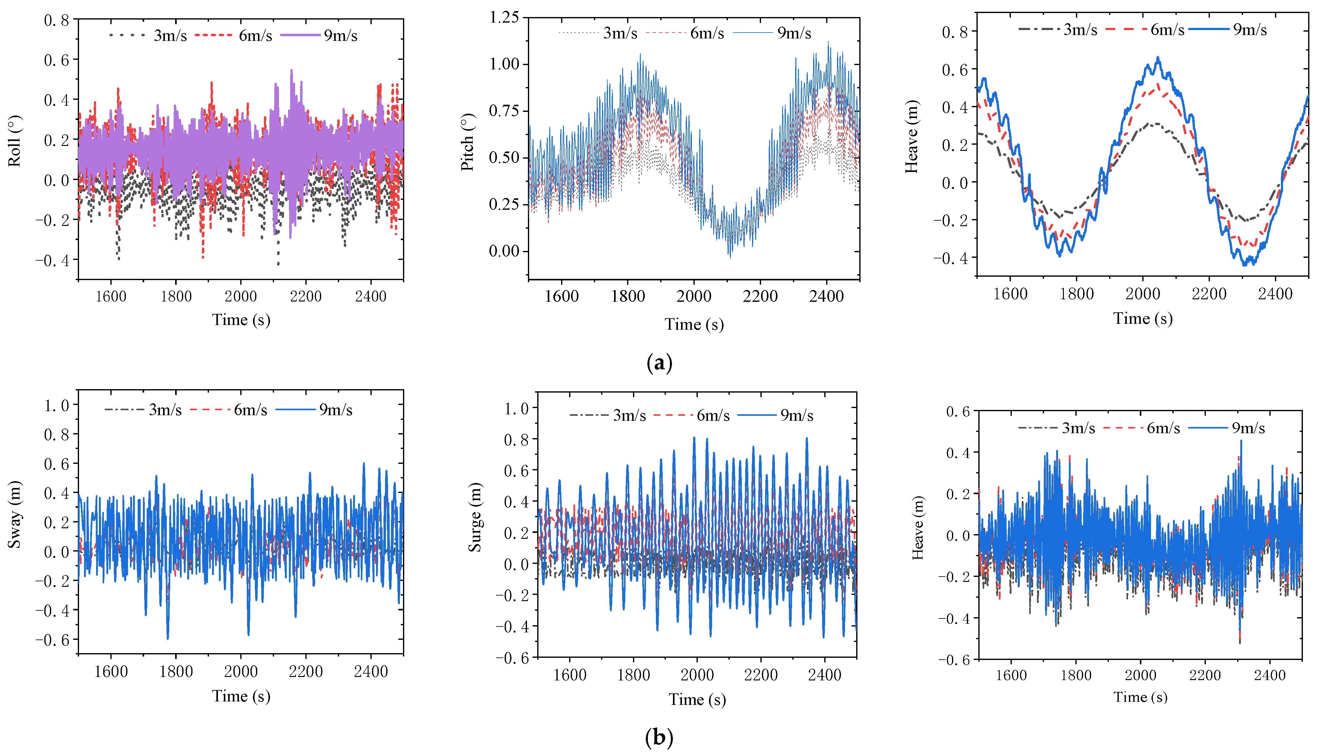
4.2.1. Wind Velocity

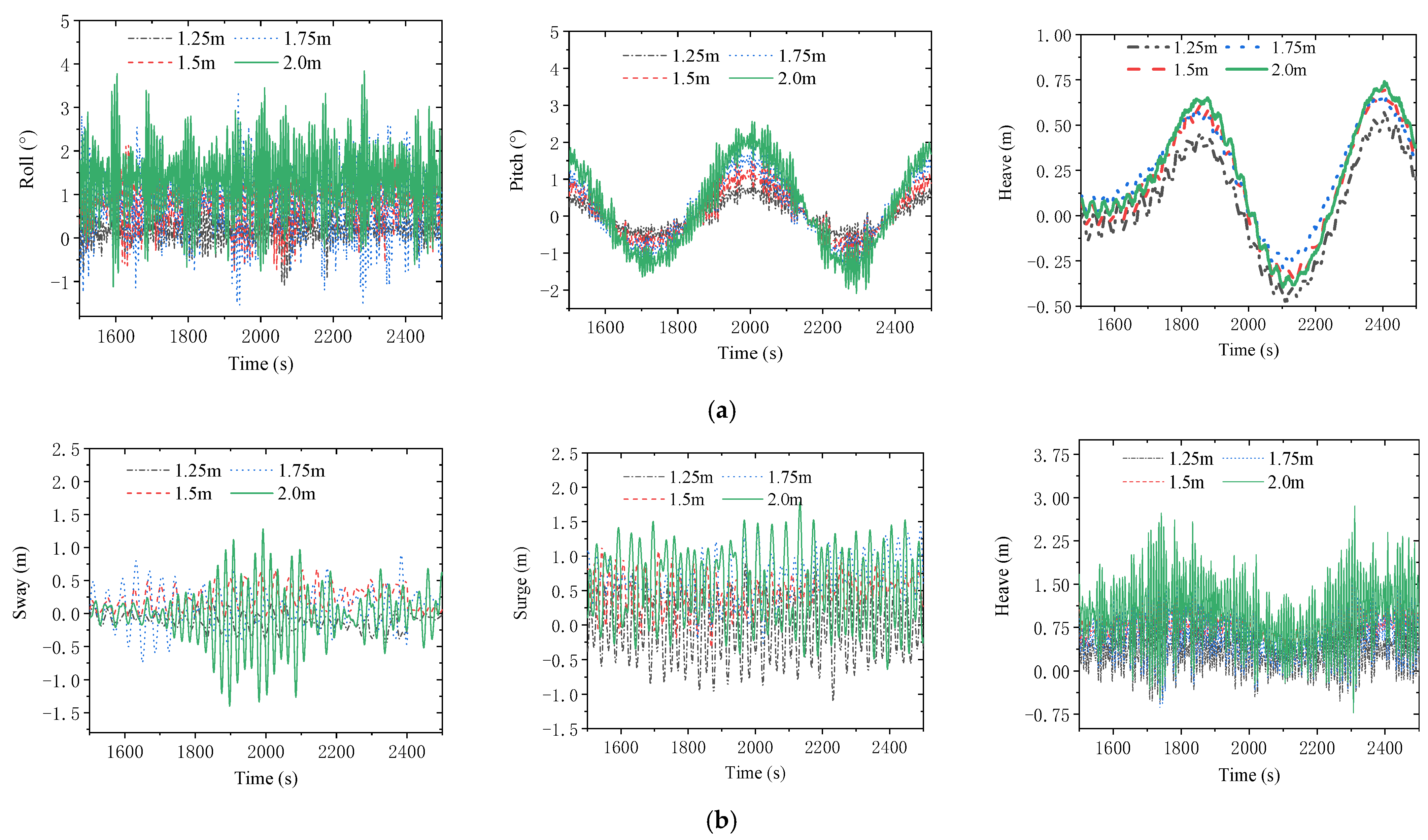
To investigate the influence of wind velocity on the motions of the floating derrick and impeller, 3 m/s, 6 m/s, and 9 m/s are selected. The motions of the ship during the lifting operation of the floating derrick under different wind velocities are shown in Figure 21a. It can be seen that the wind velocity will have significant effects on the motions of the floating derrick during the lifting operation. According to the motion trend of the time history curve in Figure 21a, it can be found that the motion amplitude of the ship increases with the increase in wind velocity in roll, pitch, and heave. Comparing the motion amplitude of the ship under wind velocities of 9 m/s and 3 m/s, the increase in the heave, roll, and pitch will achieve 59.32%, 39.56%, and 47.68%, respectively.

The motions of the lifting impeller in the sway, surge, and heave during the lifting operation under different wind velocities are shown in Figure 21b. According to the motion of the time history curves, it can be found that, in the sway, surge, and heave, the motion amplitude of the lifting object increases with the increase in the wind velocity. The increase in the maximum motion amplitude of the lifting impeller in the sway, surge, and heave under the wind velocities of 9 m/s and 3 m/s are 65.97%, 74.65%, and 21.98%, respectively. It can be found that wind velocity mainly has a great influence on the sway and surge of the lifting object.

In summary, it can be seen from the motion simulation comparison of the ship and the lifting object under different wind velocities that the wind velocity change mainly affects the pitch and heave motion of the ship under the head wave and the sway and surge motion of the lifting object. The sensitivity of the ship and the lifting object to the change in wind velocity is obvious. In the simulation calculation of the lifting operation, the influence of wind velocity may be the main one.

4.2.2. Wave Height

In order to understand the influence of wave height on the motion of the floating derrick and the impeller, wave heights of 1.25 m, 1.5 m, 1.75 m, and 2.0 m are included.

The motion roll, pitch, and heave of the floating derrick under different significant wave heights during the lifting operation are shown in Figure 22a. It can be seen that the motion amplitude of the ship roll, pitch, and heave increase with the increase in the wave height. The maximum motion amplitudes of the ship under the two wave heights of 2.0 m and 1.25 m increase by 40.78%, 59.65%, and 59.89% respectively. Comparing the effect on ship roll, the influence on the heave and pitch motion of the ship are relatively large.

The motions of the lifting impeller regarding sway, surge, and heave during the lifting operation under different significant wave heights are shown in Figure 22b. For the motions, the effect trend of sway, surge, and heave of the lifting impeller is the same, increasing with the increase in wave height. The increase in the maximum motion amplitude of the sway, surge, and heave of the lifting object under wave heights of 2.0 m and 1.25 m are 66.27%, 49.97%, and 56.19%, respectively. On the whole, it can be seen that wave height has little influence on the heave but a large influence on the motions of the sway and surge.

Comparing the motion results of the floating derrick and the impeller under different wave heights, it can be seen that the change in wave height has a great influence on the motion of the ship in heave and pitch and little influence on the motion in roll. For the lift impeller, the influence of wave height change on the heave is relatively small, but there is a large influence on the sway and surge. As the ship is under a head wave, the sloshing of the ship is transmitted to the lifting object through the sling, which aggravates the sloshing amplitude of the lifting object.

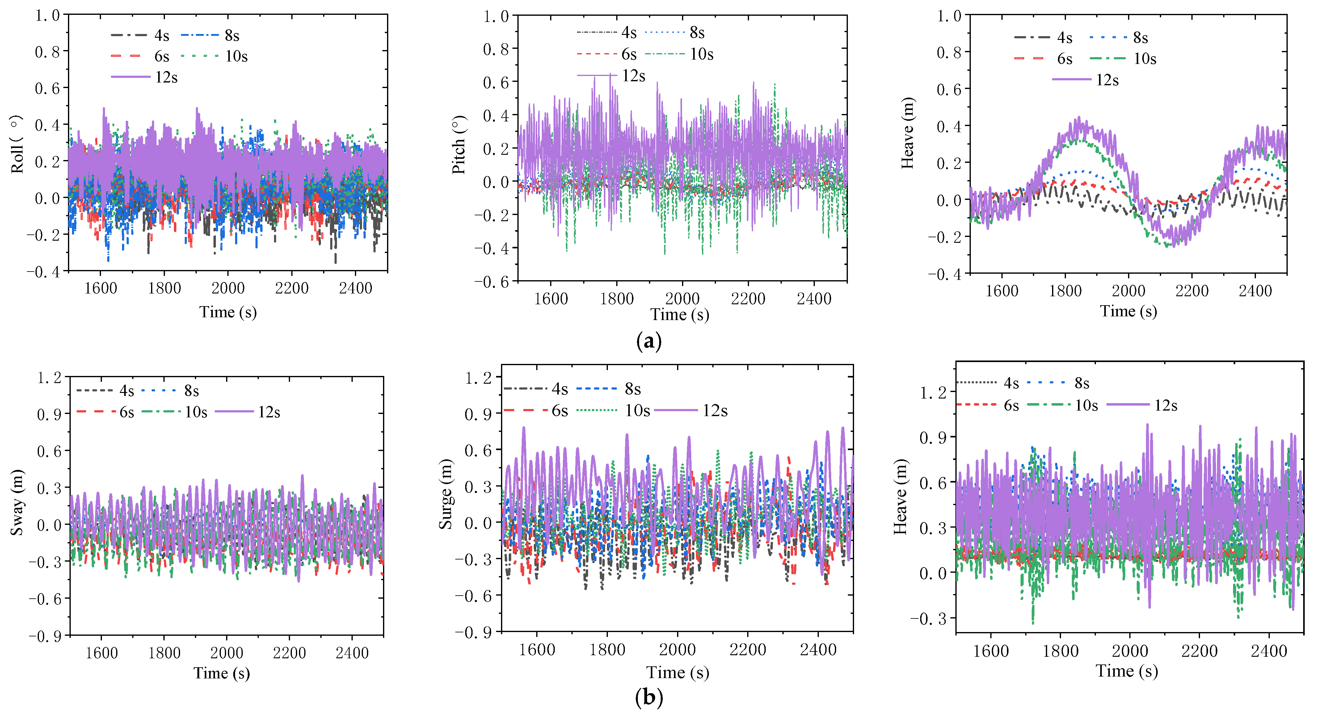
4.2.3. Spectral Peak Period

The spectral peak periods of 4 s, 6 s, 8 s, 10 s, and 12 s are included to investigate the motions of the floating derrick and impeller. The time history curves of the motions of the floating crane under different spectral peak periods are shown in Figure 23a. The large period will increase the motion roll, pitch, and heave of the floating derrick significantly.

The time history curves of the motions of the lifting impeller under different spectral peak periods are shown in Figure 23b. Comparing the results for 12 s and 9 s, the increases of the motion sway, surge, and heave are 44.76%, 67.15%, and 87.17%, respectively.

From the above results, the increase in the spectral peak periods will induce increases in the motions of the floating derrick and impeller, illustrating the ship motion’s influence on the lifting impeller.

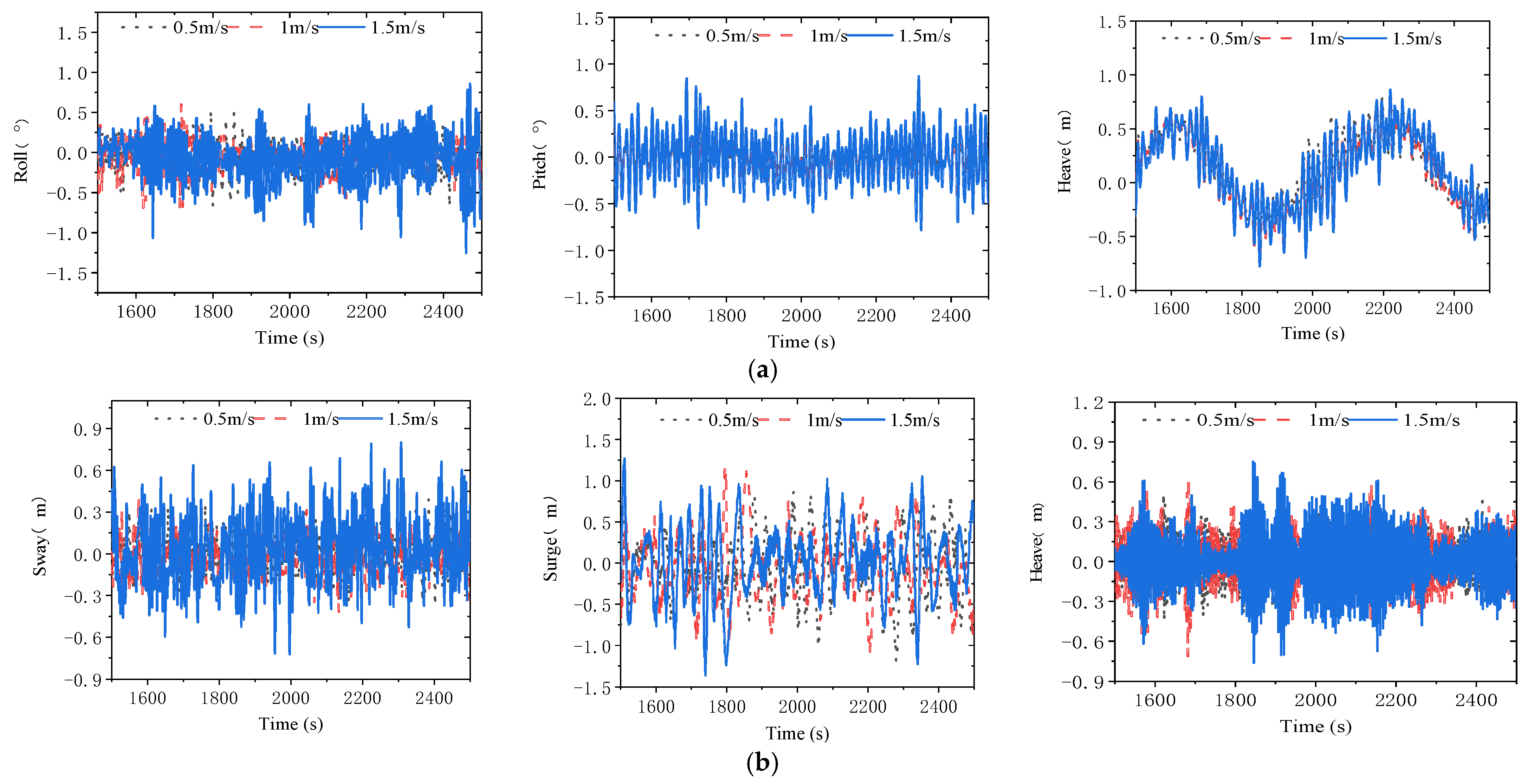
4.2.4. Current Velocity

The time history curves of the motions of the floating derrick and the lifting impeller are shown in Figure 24a,b under different current velocities of 0.5 m/s, 1 m/s, and 1.5 m/s. The increase in the current velocity will increase the motion of the ship and impeller significantly. Comparing the results at 1.5 m/s and 0.5 m/s, the motion amplitudes of the ship roll, pitch, and heave increase by 16.31%, 43.37%, and 24.34%, respectively, while the motion amplitude of the impeller sway, surge, and heave increase by 38.33%, 55.23%, and 36.27% separately. It can obviously be seen that the current velocity will affect the motions of the floating derrick and impeller.

4.3. Lifting Parameters

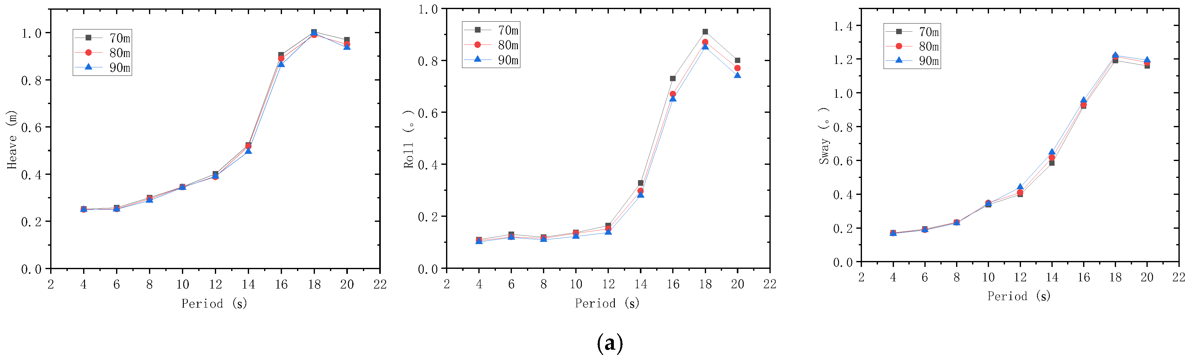
4.3.1. Lifting Heights

The heave, roll, and pitch motions of the ship and the sway, surge, and heave of the lifting are analyzed, as the lifting height increases during the lifting process. The lifting height is defined as the distance between the ship deck and the gravity center of the lifting objective.

In order to investigate the influence of the lifting height on the motion of the floating derrick and the lifting object, three lifting heights of 70 m, 80 m, and 90 m were selected for numerical simulation.

The motion responses of the floating derrick are shown in Figure 25a under different periods, as the lifting heights increase. As the periods change in the range of 4 s to 14 s, the heave and surge increase slowly with the period and increase rapidly to the peak value at the period 18 s. Afterward, the motions will reduce. The same trend happens to the roll. The lifting height has little effect on the heave and surge of the floating derrick, while the roll will increase significantly as the lifting height increases.

The motion response of the lifting impeller is shown in Figure 25b with increased lifting heights. As the lifting height increased, the surge under the lifting height of 90 m increased by 13.84% and 28.67%, compared with the results under 70 m and 80 m, but the roll increased less than 10%.

In summary, the lifting height will affect the roll of the floating derrick and surge and heave of the impeller mainly. The motion of the lifting object will be transmitted to the ship through the sling, and the motion of the ship will also increase the motion of the lifting object. The coupling force between the ship and the lifting object causes the vibration of each other, which aggravates the motion of the floating derrick and the lifting impeller.

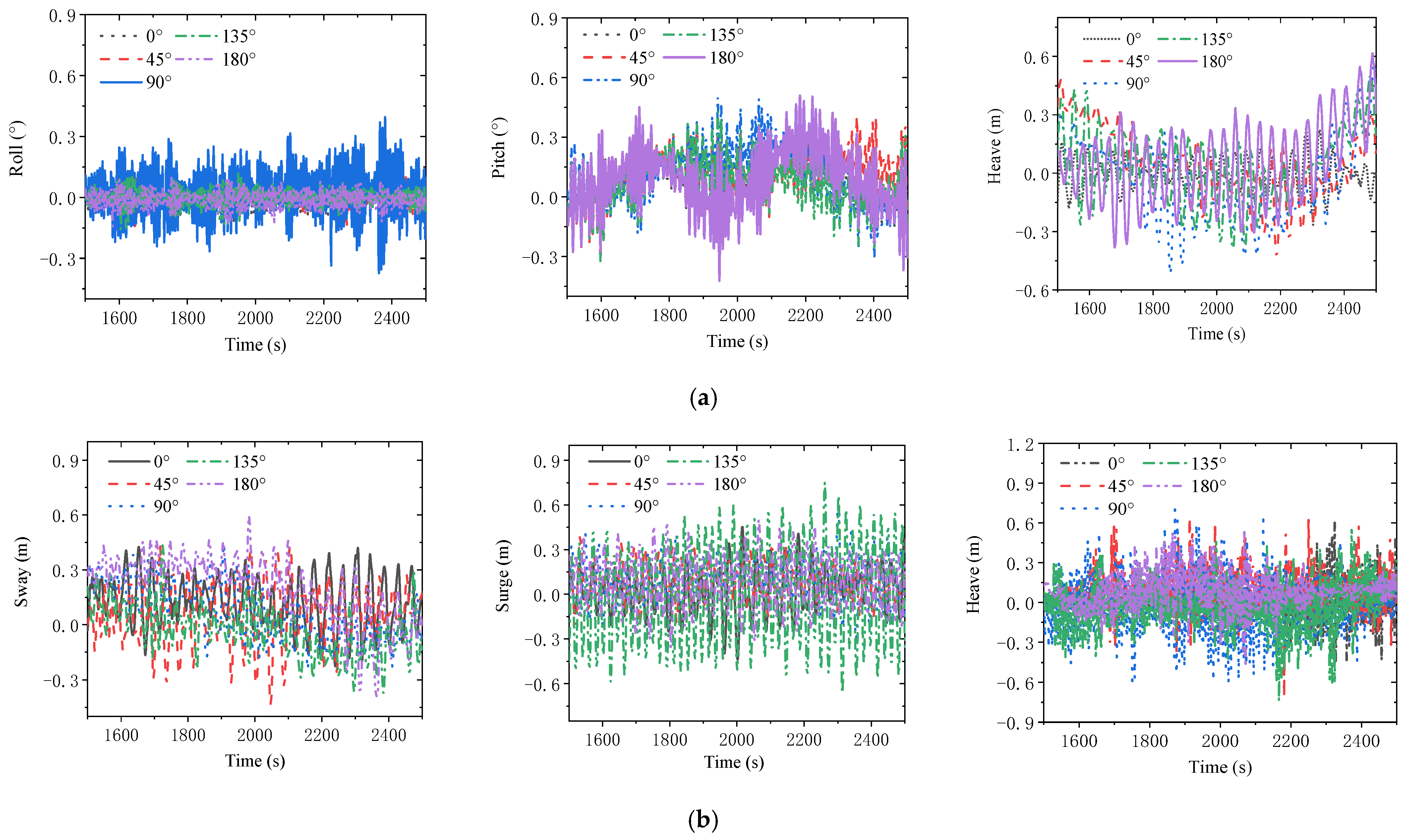
4.3.2. Boom Rotation Angle

In order to study the influence of different boom rotation angles on the floating derrick and the lifting impeller, five boom rotation angles of 0°, 45°, 90°, 135°, and 180° are selected for numerical simulation.

The motions of roll, pitch, and heave of the floating derrick are shown in Figure 14. The boom rotation angle has little effect on the motion of the roll, and the effect on the motion of the heave and surge is obvious. As the rotation angle is 180° and the lifting objective rotates to the stern, the surge amplitude of the floating derrick is the largest among the five angles. The pitch of the ship increases significantly under the action of the external load and the weight of the lifting impeller. As the rotation angle is 90° and the lifting object is on the shipboard, the roll of the ship is the largest. The lifting weight and the shaking of the lifting object induce an increase in the ship’s motions. It can be seen that the change in the boom rotation angle mainly affects the pitch of the ship, but only of small value. The boom rotation angle is not a sensitive factor to the floating derrick.

The motion sway, surge, and heave of the lifting impeller under different lifting heights are shown in Figure 26b. The boom rotation angle has little influence on the motion of the heave of the lifting impeller, and the influence on the motion of the sway and surge is obvious. The external load and the force induced by the sloshing of the floating derrick are transmitted to the lifting object through the sling, resulting in a significant increase in the motion of the lifting object. Due to the large mass of the lifting objective, the change in the gravity center aggravates the ship’s motion, which is coupled with the lifting objective through the sling, resulting in an increased motion of the lifting objective.

The change in the boom rotation angle only has some influence on the motions of the ship and the lifting impeller. The boom rotation angle is not the main influencing factor for the floating crane system. The influence of environmental parameters on the floating crane system is significant.

5. Prediction Model of Floating Crane System Based on BP Neural Network

Due to the complex and nonlinear effect of the parameters, it is not easy to predict the operation of the lifting by performing a numerical analysis for all the cases. It is appreciated to train the samples and predict the operation by machine-learning method.

5.1. Selection and Pre-Treatment of Data Samples

In the lifting process of the wind impeller using a floating derrick, the floating derrick-impeller coupling model is established. The five parameters of the wind velocity, lifting height, wave height, spectral peak period, and boom rotation angle are included to form 6125 working conditions. The extreme values of the heave, roll, and pitch of the ship are obtained, as well as the surge and heave of the lifting impeller. The working condition parameters are listed in

Table 9. Operating parameters.

Operating Condition Parameters	Value
Wave spectrum	JONSWAP
Wind spectrum	NPD
Lifting height m	65/75/80/85/90/95
Spectral peak period s	4/6/8/10/12
Wave height m	0.65/0.8/0.95/1.1/1.25/1.4/1.55
Wind velocity m/s	3/5/7/9/12
Boom rotation angle °	76/77/78/79/80

.

Using the BP neural network, which is programmed by Python, the six labels of the spectral peak period, wave height, wind velocity, boom rotation angle, and lifting height are included to build the input layer, while the extreme values of motion heave, roll, and pitch of the ship and surge and heave of the lifting impeller are the output layer. By setting the fixed number of hidden layers in the input layer and the output layer and the number of neuron nodes in each layer, the data are divided according to the ratio of 1:4. There are 4900 sets of samples randomly selected as the training data. The remaining 1225 sets of data are used as the test data of the model to verify the accuracy of the model and ensure the uniqueness and invariance of the subsequent model simulation data.

5.2. Design of Network Structure Model

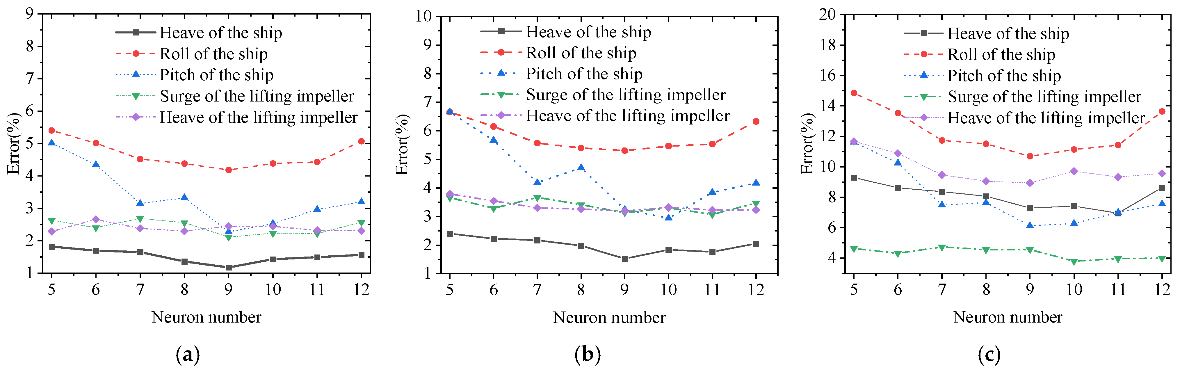
5.2.1. Determine the Number of Neurons

In order to determine the number of neurons in the hidden layer of the network model, a number of neural network training structure models are built. The activation function in the network structure adopts the default activation function in the BP neural network structure, as the tansig and purelin functions. The influence of the number of neurons on the network structure is investigated and analyzed until the number of hidden layers is determined. Eight kinds of neuron numbers, namely 5, 6, 7, 8, 9, 10, 11, and 12, were selected to build the network, as the learning rate was set to 0.01. Through the principle of controlled variables, the number of hidden layers is set to four layers, and the average absolute error We, root mean square error Wf, and average symmetric absolute error Wg are selected as the evaluation indexes of network model performance. Comparing the changes in the performance of the eight network structure models, the smaller the error, the better the performance of the network structure.

According to the error values obtained by the network training model, the average absolute error, root mean square error, and average symmetric absolute error are illustrated in Figure 27. The motions of the ship and impeller of the floating crane system are included. The network model performance evaluation index changes with the number of neurons, as shown in Figure 27. It can be seen that, with the increase in the number of neurons, the average absolute error, root mean square error, and symmetrical average absolute error of the network generally show a trend of decreasing first and then increasing. If the number of neurons is nine, the average absolute error and root mean square error are the smallest. If the number of neurons is 10, the symmetrical average absolute error is the smallest. The average absolute error is mainly around 2%, while the root mean square error is less than 5%. The symmetrical average absolute error is about 10%. When the number of neurons exceeds 10, the three error values increase. It was found that, when the number of neurons exceeded nine, the complexity of the network increased, and the training velocity of the network model structure decreased significantly. Combined with the number effect of the model performance, the number of neurons in a hidden layer is determined to be nine.

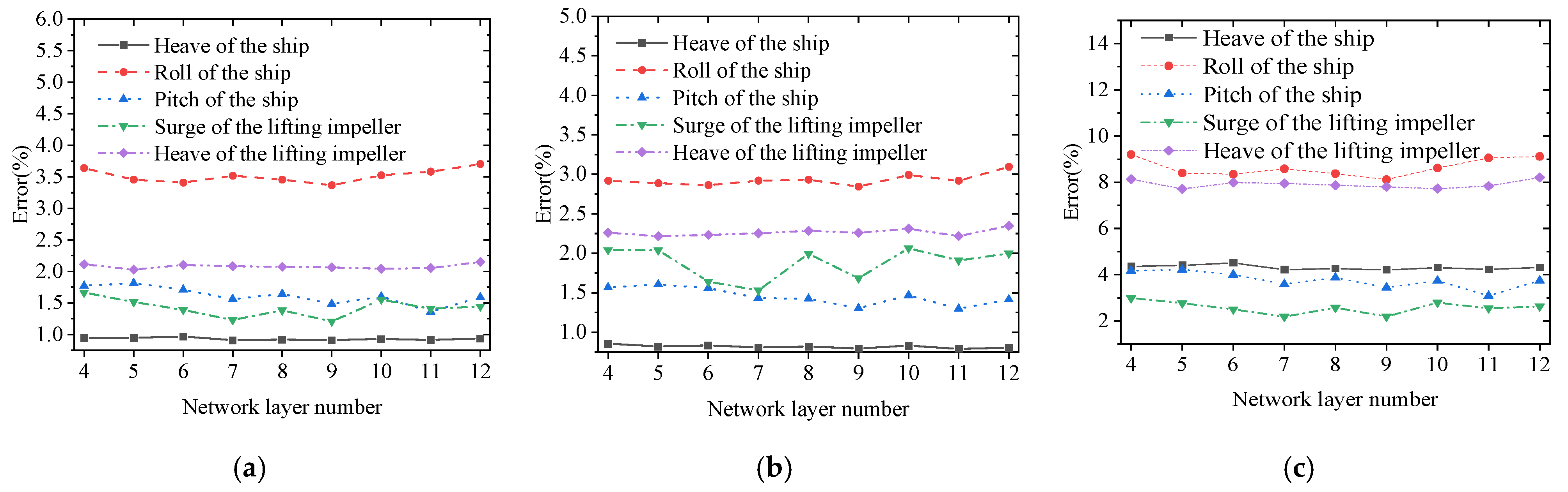
5.2.2. Determine the Number of the Network Layers

As nine neurons are in a hidden layer, the number of hidden layers in this network structure model is investigated. The training output values and original values of each network model on the motion of the ship and lifting impeller are calculated and analyzed. The average absolute error We, root mean square error Wf, and average symmetric absolute error Wg of each model are obtained, which are also used as the model performance evaluation index to assess the model performance under different hidden layers. The model performance evaluation index of the models with different hidden layers is shown in Figure 28.

It can be seen from Figure 28 that, with the increase in the number of network layers, there is a nonlinear relationship between the number of network hidden layers and the error values. When the number of network layers is nine, the three errors are close to the minimum error value. Combined with the efficiency of the model toward the training data, the model with nine hidden layers is determined as the motion prediction network model.

5.3. Model Training and Testing

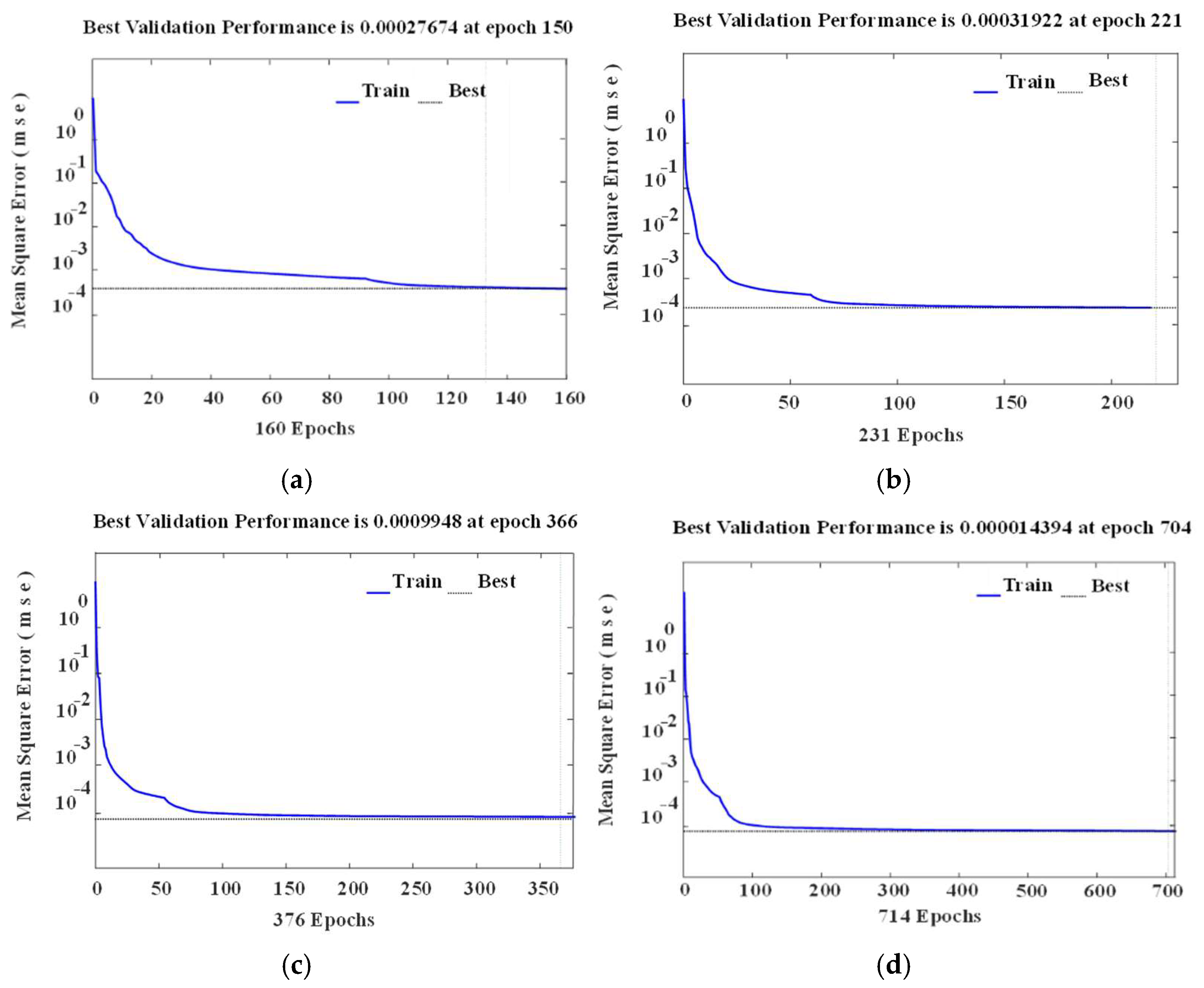
5.3.1. Network Model Training

In order to obtain a better one, the network model is trained and optimized by gradually increasing the number of samples. By comparing the model fitting errors obtained by different samples, the final training number of the model is determined. A total of 4900 samples were randomly selected from the total sample as the training data, and the remaining 1225 samples were saved as the test data. The fitting quality training process under different sample numbers, such as 1500, 2000, 3000, and 4900, is shown in Figure 29, as well as the model training error in Figure 30.

From Figure 29 and Figure 30, it can be seen that the error between the output value of the BP neural network after self-learning and the actual evaluation result is very small, which shows a good training effect of the BP neural network model built in this paper.

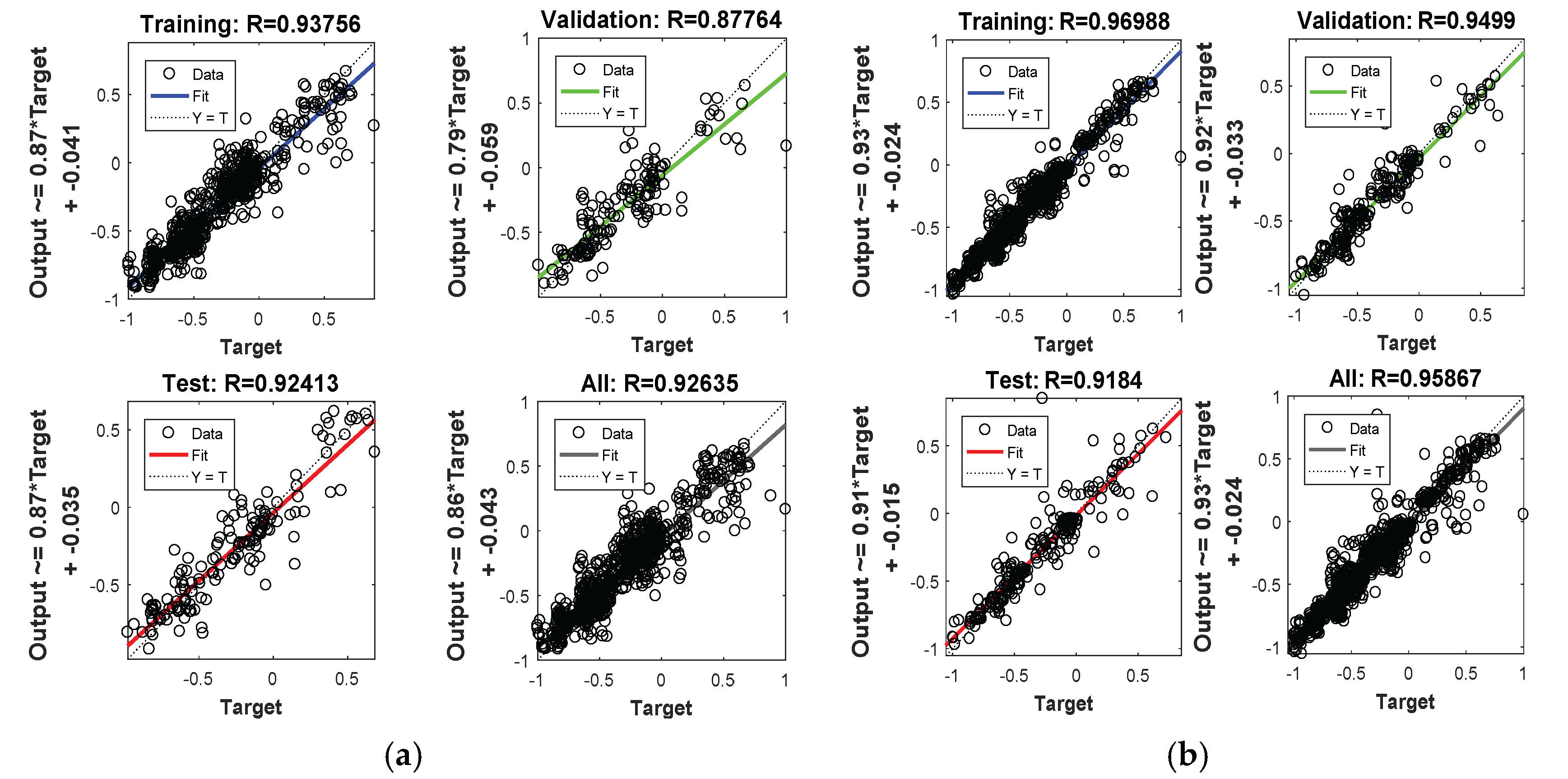
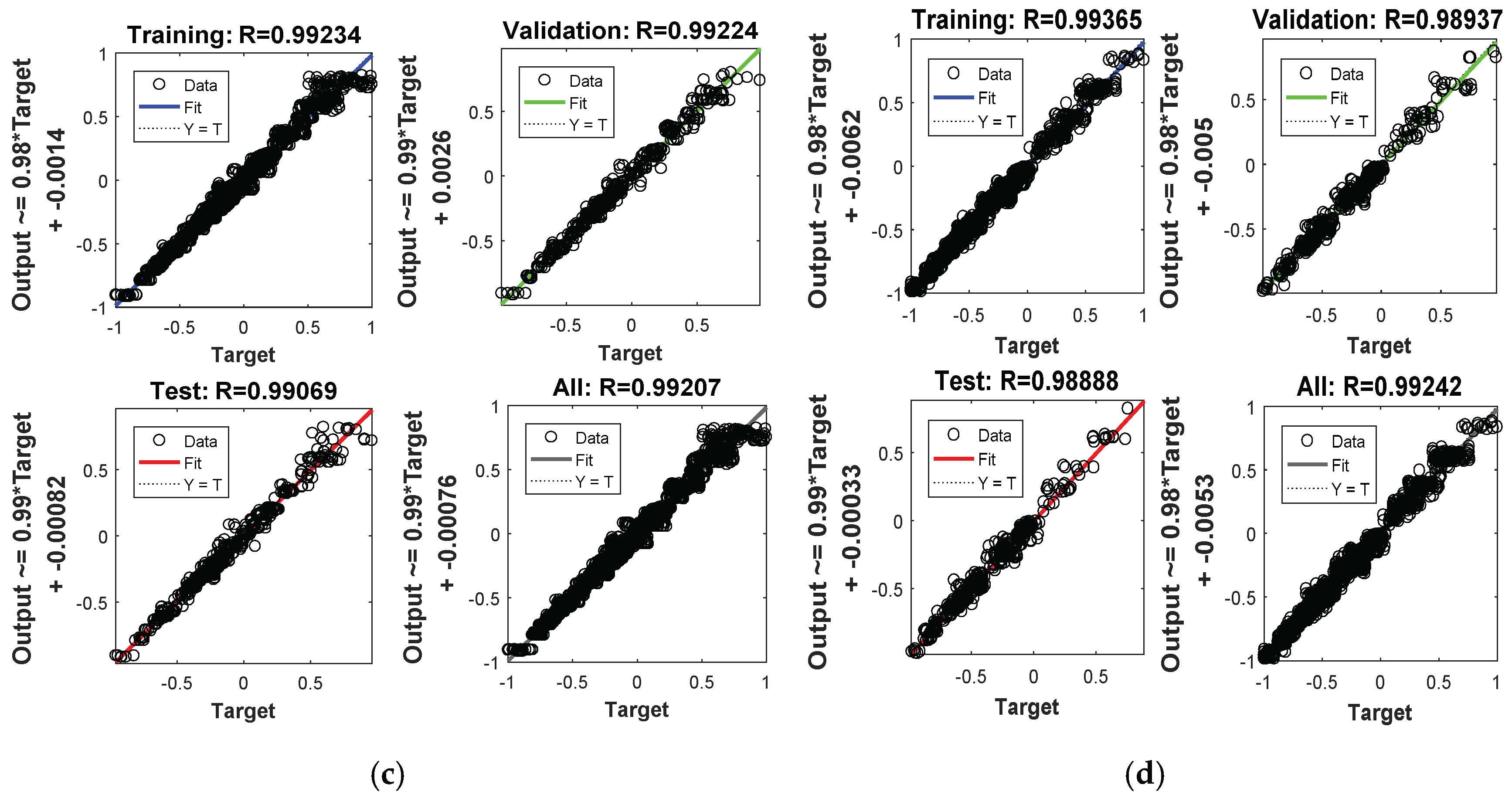
5.3.2. Network Model Testing

In order to verify the prediction of the model built above, the remaining 1225 samples are used to perform the analysis. The five features of spectral peak period, wave height, wind velocity, boom rotation angle, and lifting height are the input data. The prediction results obtained by the network model are compared with the original data. The mean absolute error We, root mean square error Wf, and symmetrical mean absolute error Wg of the predicted value and the original value are shown in

Table 10. Prediction performance evaluation index of network model.

Parameter	Heave Ship	Roll Ship	Pitch Ship	Surge Lifting Impeller	Heave Lifting Impeller
We (%)	0.0361	0.3048	0.1529	0.4114	0.2510
Wf (%)	0.1149	0.2885	0.2743	0.2509	0.3198
Wg (%)	0.0151	0.0673	0.0433	0.0048	0.0262

.

From Table 10, it can be seen that the three errors between the predicted value of the output motions of the floating crane and the lifting impeller by the network model and the original data are relatively small generally, which verifies the good performance of the prediction network model built above.

6. Prediction of Operation of the Floating Crane System

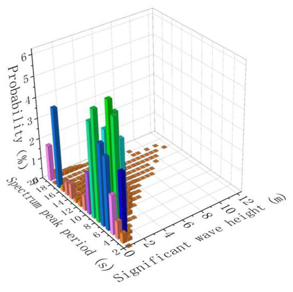
6.1. Environmental Data of a Wind Farm in the Eastern China Sea

The operation of the floating derrick lifting the impeller in this paper is performed using the neural network built in this paper on a wind farm in the East China Sea. The wave and wind data of the objective wind farm in the East China Sea in December are shown in

Table 11. Statistics of wave data on a wind farm in the East China Sea in December.

	Total	0.3	16	35	60.5	64	135.3	160	144.8	158	122	51.1	32.3	11	1.8	3	3	4	2
wave height/m	3.00–3.50											0.8	0.3
	2.50–3.00								0.8	4	5	6	4
	2.00–2.50						0.3	1	9	17	28	12	7
	1.50–2.00				0.5	2	6	15	26	35	22	6	3	6
	1.00–1.50			2	9	22	34	46	35	42	31	2	8	2	1
	0.50–1.00		5	16	38	33	59	72	68	57	36	24	10	3
	0.00–0.50	0.3	11	17	13	7	36	26	6	3		0.3			0.8	3	3	4	2
Period/s		2.25	2.75	3.25	3.75	4.25	4.75	5.25	5.75	6.25	6.75	7.25	7.75	8.25	8.75	9.25	1025	10.75	11.25

and Figure 31. The statistics of wave and wind on a wind farm in the East China Sea in December are in Figure 31. The current velocity is 1 m/s.

According to Table 11 and Figure 31a, it can be found that the significant wave height of the wind farm in December is mainly concentrated between 0.5 and 2.0 m, and the wave period distribution range is between 2 and 12 s. In Figure 31b, it can be seen that the wind velocity of the wind farm is mainly concentrated between 2 and 14 m/s. According to the network prediction model built, the wind, wave, and current characteristics of the sea environment are used. By combining different operating sea conditions, these are used as the input value of the network model. The motion response of the floating derrick and the impeller is obtained through the neural network.

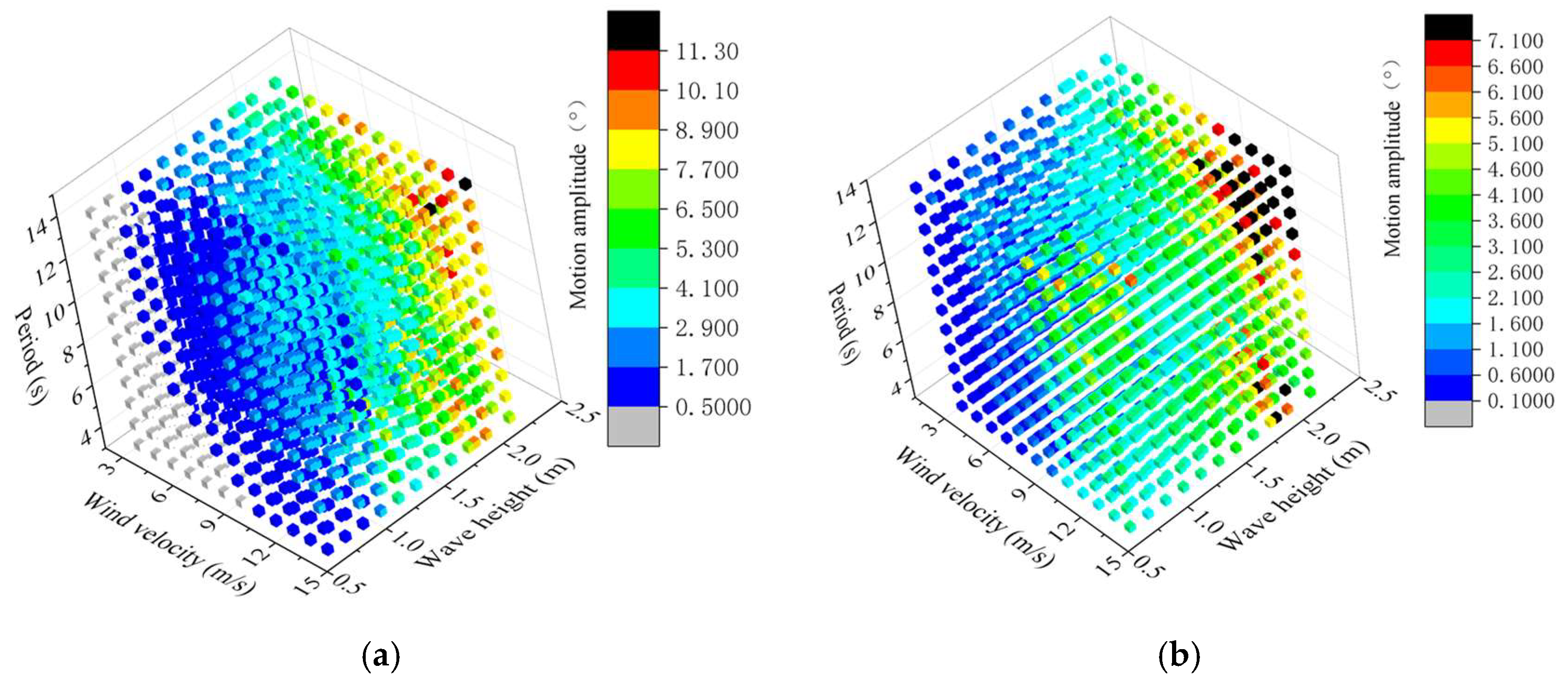
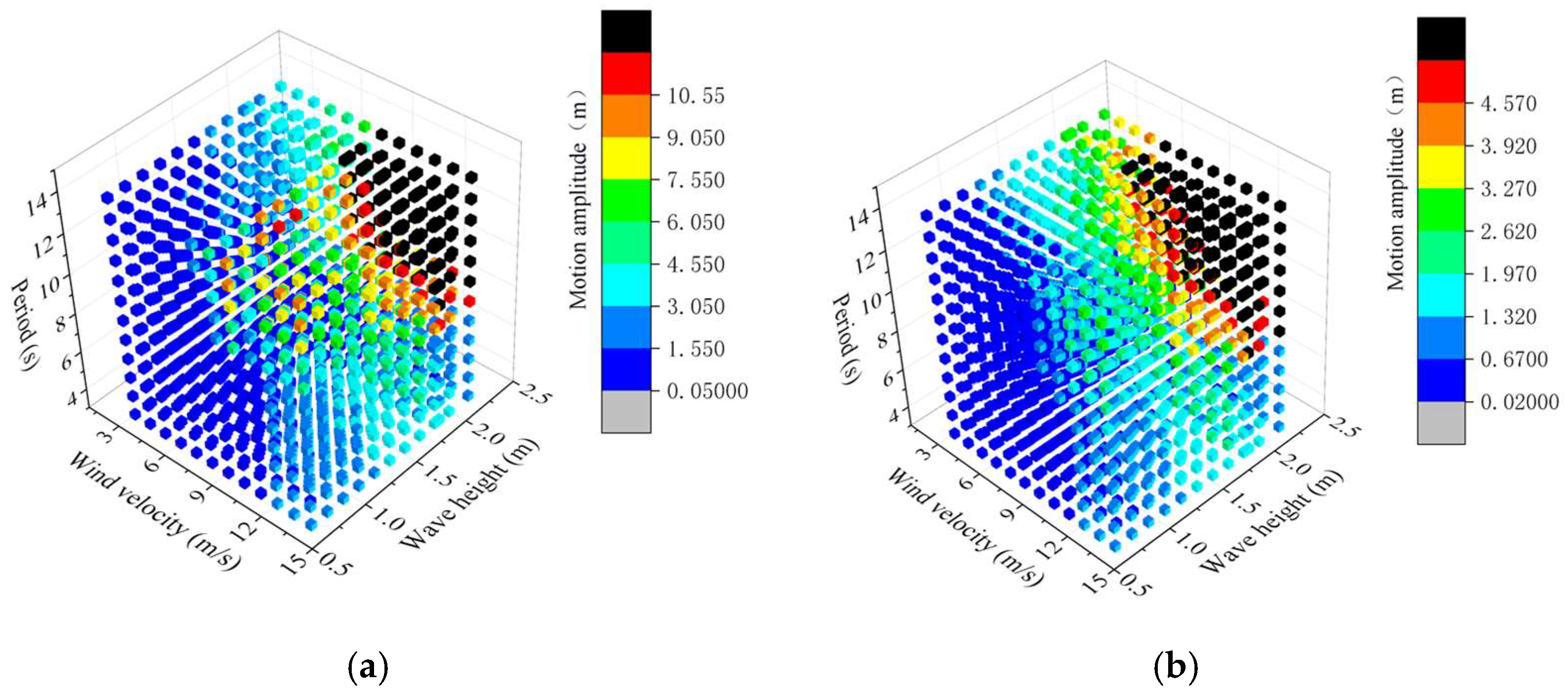
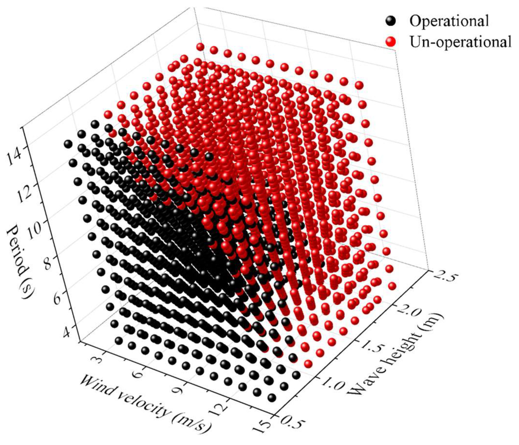
6.2. Motion Prediction and Operation Analysis

The specific input parameters are listed in

Table 12. Simulation condition parameters.

Parameters	Value
Wave height m	0.65–2.2
Wind velocity m/s	3–12
Spectral peak period s	2–12
Current velocity m/s	1.0
Lifting height m	70
Boom rotation angle °	80

according to the data in Figure 31. The motions of the floating derrick and impeller under 1728 working cases covering the objective environmental parameters are predicted by the built BP neural network model. The roll and pitch of the ship are obtained and illustrated with the wave height, period, and wind velocity in Figure 32.

According to the Rules for Lifting Appliances of Ships and Offshore Installations, the safety operation criterion for the floating derrick is that the roll is no more than 5° and the pitch no more than 2°. The influences of wind, wave, and current on the motion of the floating derrick are analyzed in Figure 32. Under the same wave period and wind velocity, the wave height has a great influence on the roll and pitch of the ship. With the increase in wave height, the operation sea conditions of the floating derrick decrease sharply.

According to the requirements of the Noble Denton Guidelines for Marine Lifting Operation [25], the safety lifting operation satisfies the following requirements: (1) the horizontal motion of the lifting object does not exceed 1.5 m and (2) the vertical motion does not exceed 0.75 m. The influences of wind, wave, and current factors on the heave and surge of the lifting impeller are analyzed, as shown in Figure 33. As the period is within 8 s and the wind velocity is no more than 6 m/s, the range of the wave height will enlarge for the safe lifting operation.

Combined with the motion criteria of the ship and lifting impeller, the operation analysis of the floating derrick lifting the impeller is performed. The results, illustrated with wind velocity, wave height, and period, are screened in Figure 34.

Each point in Figure 34 represents a result of whether the floating derrick can carry out the lifting operation safely under the corresponding wind velocity, period, and wave height. It can be seen that, if the wind velocity does not exceed 10 m/s, the period does not exceed 10 s, and the significant wave height is less than 1 m, the floating crane can safely carry out the lifting operation. In this interval, the motion amplitude of the ship and the lifting object are relatively small, which can meet the accuracy requirements of offshore wind turbine lifting and can also improve the operation efficiency of the floating derrick.

7. Conclusions

Considering the multi-body effect, the motion analysis of the floating crane system is performed, including a floating derrick, a cargo deck ship coupled with the crane, a sling, and the impeller. Based on the numerical analysis, a neural network is built by training the data obtained. Finally, the operation analysis of the floating crane system is studied by the prediction using the neural network. The following conclusions are obtained:

(1)

The cargo deck ship has a significant effect on the motion of the floating derrick, as the hydrodynamics parameters will be different considering the interaction of the cargo ship. The wind velocity under the wave in the direction of 180° mainly affects the pitch and heave motion of the ship and the sway and surge motion of the lifting. The wave height has a great influence on the sway and surge of the lifting objective. In the process of the lifting operation, the influence of the lifting height of the lifting object on the ship is mainly the pitch, and the influence on the impeller is mainly the surge and heave motion. The boom rotation angle is not the main influencing factor for the floating crane system. The coupling effect of the floating derrick with the lifting impeller is obvious, as the sloshing of the ship is transmitted to the lifting object through the sling, which aggravates the sloshing amplitude of the lifting object;

(2)

The BP neural network for the floating crane motion response prediction model is built, based on the evaluation indexes of the model performance under different parameters. It is determined that the neural network model with nine hidden layers and nine neurons in each hidden layer can give a good prediction with a small error. The BP neural network is verified to be effective and feasible for predicting the motions of the floating crane system;

(3)

Based on the environmental characteristics, the motions of the 1728 working cases are generated by the BP neural network. Combined with the Rules for Lifting Appliances of Ships and Offshore Installations [24] and the Noble Denton Guidelines for Marine Lifting Operation [25], the operation analysis of the floating crane system is performed. As the wind velocity does not exceed 10 m/s, the period does not exceed 10 s, and the significant wave height is within 1 m, the floating crane ship can safely carry out the lifting operation, and its operation efficiency will be improved accordingly.

References

1. Ye, J.; Li, C.; Wen, W.; Zhou, R.; Reppa, V. Deep Learning in Maritime Autonomous Surface Ships: Current Development and Challenges. J. Mar. Sci. Appl. 2023, 22, 584–601. [Google Scholar] [CrossRef]
2. Kristensen, H.O. Statistical Analysis and Determination of Regression Formulas for Main Dimensions of Container Ships Based on IHS Fairplay Data; University of Southern Denmark: Odense, Denmark, 2013. [Google Scholar]
3. Papanikolaou, A. Ship Design; Springer: Dordrecht, The Netherlands, 2014. [Google Scholar] [CrossRef]
4. Gurgen, S.; Altın, İ.; Ozkok, M. Prediction of Main Particulars of a Chemical Tanker at Preliminary Ship Design Using Artificial Neural Network. Ships Offshore Struct. 2018, 13, 459–465. [Google Scholar] [CrossRef]
5. Cepowski, T.; Chorab, P. Determination of Design Formulas for Container Ships at the Preliminary Design Stage Using Artificial Neural Network and Multiple Nonlinear Regression. Ocean Eng. 2021, 238, 109727. [Google Scholar] [CrossRef]
6. Jeon, M.; Noh, Y.; Shin, Y.; Lim, O.K.; Lee, I.; Cho, D. Prediction of Ship Fuel Consumption by Using an Artificial Neural Network. J. Mech. Sci. Technol. 2018, 32, 5785–5796. [Google Scholar] [CrossRef]
7. Kaplan, P. A Study of Prediction Techniques for Aircraft Carrier Motions at Sea. J. Hydronautics 1969, 3, 121–131. [Google Scholar] [CrossRef]
8. Triantafyllou, M.; Bodson, M.; Athans, M. Real Time Estimation of Ship Motions Using Kalman Filtering Techniques. IEEE J. Ocean Eng. 1983, 8, 9–20. [Google Scholar] [CrossRef]
9. Hui, L.; Chen, G.; Li, X.F. Analysis and Prediction of Ship Roll Motion Based on the Theory of Wavelet Transform. J. Dalian Marit. Univ. 2010, 36, 5–8. [Google Scholar] [CrossRef]
10. Ma, J.; Li, G. Time Series Prediction of Ship Rolling. J. Beijing Inst. Mach. 2006, 4–7. [Google Scholar] [CrossRef]
11. Li, G.; Kawan, B.; Wang, H.; Zhang, H. Neural-Network-Based Modeling and Analysis for Time Series Prediction of Ship Motion. Ship Technol. Res. 2017, 64, 30–39. [Google Scholar] [CrossRef]
12. Gao, M.; Shi, G.; Li, S. Online Prediction of Ship Behavior with Automatic Identification System Sensor Data Using Bidirectional Long Short-Term Memory Recurrent Neural Network. Sensors 2018, 18, 4211. [Google Scholar] [CrossRef] [PubMed]
13. Duan, W.-Y.; Huang, L.-M.; Han, Y.; Zhang, Y.-H.; Huang, S. A Hybrid AR-EMD-SVR Model for The Short-Term Prediction of Nonlinear and Non-Stationary Ship Motion. J. Zhejiang Univ.-SCIENCE A 2015, 16, 562–576. [Google Scholar] [CrossRef]
14. Khan, A.; Bil, C.; Marion, K.E. Ship Motion Prediction for Launch and Recovery of Air Vehicles. In Proceedings of the OCEANS 2005 MTS/IEEE, Washington, DC, USA, 17–23 September 2005; Volume 2793, pp. 2795–2801. [Google Scholar]
15. Cha, J.-H.; Roh, M.-I.; Lee, K.-Y. Dynamic Response Simulation of a Heavy Cargo Suspended by a Floating Crane Based on Multibody System Dynamics. Ocean Eng. 2010, 37, 1273–1291. [Google Scholar] [CrossRef]
16. Van Trieu, P. Combined Controls of Floating Container Cranes. In Proceedings of the 2015 International Conference on Control, Automation and Information Sciences (ICCAIS), Changshu, China, 29–31 October 2015. [Google Scholar]
17. Ardhiansyah, F.; Prastianto, R.W.; Murdjito; Suastika, K.; Nugroho, S. Dynamic Response of Floating Crane During Lifting Operation: A Parametric Study. In Applied and Computational Mathematics; Springer Proceedings in Mathematics & Statistics; Springer Nature: Singapore, 2024; Volume 455. [Google Scholar] [CrossRef]
18. Nam, B.W.; Kim, N.W.; Hong, S.Y. Experimental and Numerical Study on Coupled Motion Responses of a Floating Crane Vessel and a Lifted Subsea Manifold in Deep Water. Int. J. Nav. Archit. Ocean Eng. 2017, 9, 552–567. [Google Scholar] [CrossRef]
19. Soner, O.; Akyuz, E.; Celik, M. Statistical Modelling of Ship Operational Performance Monitoring Problem. J. Mar. Sci. Technol. 2019, 24, 543–552. [Google Scholar] [CrossRef]
20. An, J.; Yu, Y.; Cao, W.; Wu, M. Load Distribution and Optimization Method for Cooperative Lifting of Double Cranes Considering the Minimal Lifting Consumption. In Proceedings of the 33rd Chinese Control Conference, Nanjing, China, 28–30 July 2014; pp. 2969–2974. [Google Scholar]
21. Cheng, N.; Chen, L.; Zeng, D. Ship Energy Efficiency Prediction Method Based on Data Mining Techniques. In Proceedings of the 2024 3rd Conference on Fully Actuated System Theory and Applications (FASTA), Shenzhen, China, 10–12 May 2024. [Google Scholar]
22. Gao, Z. Research in Data Mining Technology of Ship Intelligent Energy Efficiency Management. Master’s Thesis, Dalian Maritime University, Dalian, China, 2019. [Google Scholar]
23. DNV. User Guide for SIMA; SINTEF Ocean and DNV: Oslo, Norway, 2022. [Google Scholar]
24. China Classification Society. Rules for Lifting Appliances of Ships and Offshore Installations; China Communications Press: Beijing, China, 2007. [Google Scholar]
25. GL Noble Denton. Guidelines for Marine Lifting Operations; Technical Policy Board: Berlin, Germany, 2010. [Google Scholar]
26. Jonkman, J.; Butterfield, S.; Musial, W.; Scott, G. Definition of a 5-MW Reference Wind Turbine for Offshore System Development; National Renewable Energy Laboratory: Golden, CO, USA, 2009. [Google Scholar]
27. Luo, X. Numerical Simulation and Experimental Study on Motion Responses of Lanjiang Crane Vessel Coupling System in Heading Waves. Master’s Thesis, Tianjin University, Tianjin, China, 2018. (In Chinese). [Google Scholar]
Figure 1. Flowchart of the operation analysis of the floating derrick lifting the impeller.
Jmse 12 02136 g001
Figure 2. Model of wind turbine impeller.
Jmse 12 02136 g002
Figure 3. Definition of coordinate for two adjacent floating bodies.
Jmse 12 02136 g003
Figure 4. Motion analysis diagram of floating derrick and lifting objective.
Jmse 12 02136 g004
Figure 5. Structure diagram of BP neural network.
Jmse 12 02136 g005
Figure 6. Layout of the moored floating derrick and the deck cargo ship.
Jmse 12 02136 g006
Figure 7. Model of floating crane and impeller.
Jmse 12 02136 g007
Figure 8. Numerical model and experiment model of double floating body system. (a) Numerical model of double floating body system. (b) Experiment model of double floating body system.
Jmse 12 02136 g008
Figure 9. The motion response of the two barges in double floating body system by experiment and numerical method. (a) Maximum value results of barge 1. (b) Minimum value results of barge 1. (c) Error of barge 1. (d) Maximum value results of barge 2. (e) Minimum value results of barge 2. (f) Error of barge 2.
Jmse 12 02136 g009
Figure 10. Added mass of the floating derrick. (a) Surge, (b) sway, (c) heave, (d) roll, (e) pitch, and (f) yaw.
Jmse 12 02136 g010
Figure 11. Added mass of the deck cargo ship. (a) Surge, (b) sway, (c) heave, (d) roll, (e) pitch, and (f) yaw.
Jmse 12 02136 g011aJmse 12 02136 g011b
Figure 12. Radiation damping of the floating derrick. (a) Surge, (b) sway, (c) heave, (d) roll, (e) pitch, and (f) yaw.
Jmse 12 02136 g012
Figure 13. Radiation damping of the cargo ship. (a) Surge, (b) sway, (c) heave, (d) roll, (e) pitch, and (f) yaw.
Jmse 12 02136 g013
Figure 14. RAOs of the floating derrick. (a) Surge, (b) sway, (c) heave, (d) roll, (e) pitch, and (f) yaw.
Jmse 12 02136 g014aJmse 12 02136 g014b
Figure 15. RAOs of the cargo ship. (a) Surge, (b) sway, (c) heave, (d) roll, (e) pitch, and (f) yaw.
Jmse 12 02136 g015
Figure 16. First-order wave force of the floating derrick. (a) Surge, (b) sway, (c) heave, (d) roll, (e) pitch, and (f) yaw.
Jmse 12 02136 g016
Figure 17. First-order wave force of the cargo ship. (a) Surge, (b) sway, (c) heave, (d) roll, (e) pitch, and (f) yaw.
Jmse 12 02136 g017
Figure 18. Second-order wave force of the floating derrick. (a) Surge, (b) sway, (c) heave, (d) roll, (e) pitch, and (f) yaw.
Jmse 12 02136 g018
Figure 19. Second-order wave force of the cargo ship. (a) Surge, (b) sway, (c) heave, (d) roll, (e) pitch, and (f) yaw.
Jmse 12 02136 g019aJmse 12 02136 g019b
Figure 20. Joint frequency distribution of the wave period and significant wave height in East China Sea.
Jmse 12 02136 g020
Figure 21. Time history curves of the motions of the floating derrick and the impeller under different wind velocities. (a) The floating derrick, (b) the impeller.
Jmse 12 02136 g021
Figure 22. Time history curve of the floating derrick and the lifting impeller under different wave heights. (a) The floating derrick, (b) the impeller.
Jmse 12 02136 g022
Figure 23. Time history curve of motions of the floating derrick and impeller under different spectral peak periods. (a) The floating derrick, (b) the impeller.
Jmse 12 02136 g023
Figure 24. Time history curves of the motions of floating derrick and impeller under different current velocities. (a) The floating derrick, (b) the impeller.
Jmse 12 02136 g024
Figure 25. Amplitude of motion response of floating derrick and impeller under different lifting heights. (a) The floating derrick. (b) The lifting impeller.
Jmse 12 02136 g025aJmse 12 02136 g025b
Figure 26. Time history curves of the motion of the floating derrick and impeller under different boom rotation angles. (a) The floating derrick, (b) the impeller.
Jmse 12 02136 g026
Figure 27. The change in model performance evaluation index under different numbers of neurons. (a) We. (b) Wf. (c) Wg.
Jmse 12 02136 g027
Figure 28. The change in model performance evaluation index under different numbers of network layers. (a) We. (b) Wf. (c) Wg.
Jmse 12 02136 g028
Figure 29. Model training performance under different samples: (a) 1500 sets of data, (b) 2000 sets of data, (c) 3000 sets of data, and (d) 4900 sets of data.
Jmse 12 02136 g029aJmse 12 02136 g029b
Figure 30. Model training errors under different samples: (a) 1500 sets of data, (b) 2000 sets of data, (c) 3000 sets of data, and (d) 4900 sets of data.
Jmse 12 02136 g030
Figure 31. Statistics of wave and wind on a wind farm in the East China Sea in December. (a) The wave. (b) The wind.
Jmse 12 02136 g031
Figure 32. The amplitude of the roll and pitch of the floating derrick. (a) Roll and (b) pitch.
Jmse 12 02136 g032
Figure 33. The amplitude of surge and heave of the lifting impeller. (a) Surge and (b) heave.
Jmse 12 02136 g033
Figure 34. Operation analysis of the floating crane system.
Jmse 12 02136 g034