Analytical Modeling of the Lazy-Wave Hydrogen Production Riser (HPR) with Incorporation of Seabed Interaction in the Touchdown Zone

Abstract

Hydrogen production risers (HPRs) connected to floating offshore wind turbines (FOWTs) must be properly configured to minimize both the top-end tension at the hang-off point and the oscillation amplitude in the touchdown zone (TDZ) under environmental loads. One of the best riser configurations to meet these requirements is the lazy-wave configuration, where the riser is lifted midway by buoyancy tanks to create a negative curvature, mitigating the motion dependency of the catenary part and the TDZ. Analytical solutions can be effectively used in riser optimization and configuration studies, where a large number of analyses need to be conducted iteratively. In this paper, an analytical model for HPRs has been developed by combining different approaches for the hanging and touchdown zones to improve the accuracy and continuity of shear force, bending moment, and axial tension distribution along the riser, which are the key parameters governing fatigue damage accumulation in the TDZ. Modified catenary equations were used for the hanging part, and a boundary layer model was implemented in the touchdown zone to model the seabed interaction, preventing stress discontinuity between the two sections. The model was used to assess a case study and compared with numerical simulations to ensure accuracy and viability. The proposed model can be used in daily engineering practice for preliminary investigations and optimization studies of HPRs.

1. Introduction

Hydrogen can release a higher heat per unit mass compared to gasoline, which makes it a highly efficient energy source. In addition, the combustion of this attractive element that has been abundant on Earth and around it results in the production of only water vapor, rendering it a clean and sustainable source of energy [1]. In 2022, the International Energy Agency (IEA) predicted an increase in demand for hydrogen production to around 115 million tons by 2030, where less than 2 million tons will be provided by new applications. The global hydrogen market is expected to experience a substantial surge by 2050, reaching a range of 600–650 million tons, which would be more than 20% of the world’s energy demand. However, to optimize its viability, there is a concurrent requirement for achieving lower costs, enhancing production efficiency, and identifying viable methods for storage and transportation. The electrolysis process is widely seen as a promising avenue for producing hydrogen with minimal CO₂ emissions, especially when powered by green sources like nuclear and renewable energies, such as offshore wind turbines [2]. Hydrogen can be generated either centrally within the offshore wind farm or at each individual offshore wind turbine, eliminating the necessity for high-voltage cables [3]. Multi-layer flexible risers (MLFRs) with different configurations, including catenary or lazy-wave profiles, may be used as hydrogen production risers (HPRs) for transferring the hydrogen from the floating wind turbine to the seabed lines [4]. Flexible lazy-wave risers (FLWRs) are extremely exposed to wave- and current-induced oscillations and consequently to fatigue loads, with two critical hot spots: the riser attachment point to the FOWT and the touchdown zone, where the riser comes into cyclic contact with the seabed soil. In practice, optimization studies aim to identify the ideal HPR configuration to minimize fatigue damage at both the hang-off point and the touchdown zone (TDZ). Analytical models are valuable tools in these studies, offering a quick assessment of stress profiles across the HPR. The influence of the riser–seabed interaction on stress distribution and HPR fatigue is a key factor that can result in stress discontinuities in the analytical model if not properly modeled [5]. The simple catenary profiles that have been widely used in steel risers can be an option for HPRs as well. However, the catenary configuration may cause a high axial tension load at the hang-off point and large oscillation amplitudes in the touchdown zone, which in turn reduces the fatigue life. Recent research has extensively explored the static and dynamic behaviors of deepwater riser systems, with a focus on the complexity of the deepwater riser problem in terms of improving their performance and reliability in challenging marine environments. However, the industry is still in need of an analytical model for FLWRs with more accurate seabed interaction models to account for the riser profile in the TDZ, which is a hot spot for fatigue damage accumulation, and is a key objective of the current study. Despite the fatigue performance of FLWRs with the incorporation of nonlinear seabed interaction effects having been rarely investigated in the literature, the mechanical performance of SLWRs has been well investigated.

Wang et al. (2024) introduced a simplified static model based on catenary theory and static equilibrium to aid the initial design of SLWR configurations [6]. The model suggests that each section of the SLWR conforms to a hyperbolic function. A case study conducted at a water depth of 1500 m examined critical factors such as hang-off angle, elevation, and content density. The findings offer valuable insights for future detailed design and engineering phases.

Another study presents a comparative dynamic analysis of steel catenary risers (SCRs) and lazy-wave steel catenary risers (LWRs) within a coupled platform–mooring–riser system under internal solitary wave (ISW) conditions [7]. Utilizing a self-developed numerical model, the study examines responses to ISWs alone and combined ISWs and random waves (RWs). The results indicate that different riser configurations have minimal impact on platform response or mooring top tension. However, LWRs exhibit larger motion characteristics and responses over time due to their complex configuration, particularly near the ISW interface, where notable changes in horizontal tension, shear force, and bending moment are observed.

The steel lazy-wave riser (SLWR) is analyzed using nonlinear large-deformation beam theory in deep water by Chen et al. (2022) [8]. Equilibrium equations are derived via the minimum total potential energy principle. A numerical iterative method handles riser–seabed interaction efficiently, facilitating parameter optimization. The study outlines SLWR configuration and characteristics, explores their performance under various conditions, and outlines a methodology for parameter selection and optimal configuration determination. Validation using OrcaFlex software (10.2a) confirms the results. Static analyses highlight how water depth, span, upper catenary length, extreme sea conditions, and vessel motion impact riser configuration, tension, bending moment, and shear force distribution.

Cheng et al. (2016) combined experimental and numerical methods to study the response of steel lazy-wave risers in extreme environmental conditions [9]. Conducted by the DeepStar^® consortium, this research involved model scale tests to analyze the riser’s hydrodynamic behavior under forced oscillatory and random wave motions. Deformations were measured using fiber Bragg grating (FBG) strain sensors and force transducers, capturing both in-plane and out-of-plane responses. Numerical simulations focusing on in-plane responses were compared with experimental data using typical hydrodynamic coefficients such as added mass and drag. Adjustments to these coefficients improved the accuracy of the simulations. The study highlights the effectiveness of combining experimental and numerical approaches for understanding riser behavior and discusses methodologies for test data post-processing and riser modeling.

Jhingran et al. (2012) investigated the implications of buoyancy spacing on fatigue damage caused by vortex-induced vibrations (VIVs) in steel lazy-wave risers (SLWRs), particularly in deepwater environments with strong currents [10]. Given the increasing challenges in designing risers with sufficient strength and fatigue life for deeper waters, the study highlighted the SLWR concept’s promise and its associated challenges. The research, conducted by Shell Oil Company at the Marintek Ocean Laboratory in Norway, involved state-of-the-art experiments with a 38 m-long pipe to examine the effects of buoyancy spacing on VIV response. The study utilized sections with diameters of 30 mm and 80 mm to simulate the riser and buoyancy, respectively. The findings provided crucial design insights into effective buoyancy module sizing and placement to mitigate VIV-induced fatigue damage in SLWRs.

Wang et al. (2019) developed an analytical model to analyze the transfer process of deepwater steel lazy-wave risers (SLWRs) on an elastic seabed, addressing the nonlinearity introduced by buoyancy modules during installation [11]. The SLWR is favored for deepwater installations due to its superior service performance, but the transfer process poses significant challenges. This model considers the elastic seabed and boundary-layer phenomena to handle the three distinct stages of the transfer process. The reliability of the model was verified through a typical SLWR transfer process analysis, examining riser configurations and critical mechanical parameters affecting riser performance. This study offers a practical reference for the design and analysis of SLWR installations, emphasizing the importance of accurate modeling in ensuring installation feasibility and performance.

Wang et al. (2014) addressed the challenges of high hang-off tension and fatigue damage at the touchdown point (TDP) in deepwater steel lazy-wave risers (SLWRs) (the TDP refers to a single point on the riser that is located in a riser length zone, referred to as the TDZ) [12]. The study proposed a model based on nonlinear large deformation beam theory to simulate the suspended part of SLWRs, offering greater accuracy than previous small deformation beam or catenary theories. This model accounts for the riser’s bending stiffness and rapid changes in inclination angle and includes pipe–soil interaction for simulating the TDP. Using the finite difference method, the numerical solutions showed good agreement with the OrcaFlex results. Parametric analyses examined the influences of buoyancy section length, upper section length, and soil stiffness on static performance, providing a foundational reference for the dynamic analysis of deepwater SLWRs.

Wang and Duan (2015) developed a nonlinear model for deepwater steel lazy-wave risers (SLWRs) that incorporates the effects of pipe–soil interaction, ocean current, and internal flow on riser configuration and static performance [13]. The model uses conventional small deformation beam theory for the seabed portion and large deformation beam theory for the suspended section, addressing the challenges of large hang-off tension and fatigue damage at the touchdown point (TDP). The finite difference method was used to obtain numerical results, and comprehensive parametric analyses were conducted to assess the impacts of ocean current and internal flow. This model provides valuable insights and serves as a significant reference for the design and analysis of deepwater SLWRs.

Ruan et al. (2019) proposed a simplified solution to estimate the static stress range of a deepwater steel lazy-wave riser (SLWR) considering vessel slow drift motion and ocean current [14]. Their results indicated that due to the TDP relocation caused by the vessel slow motion, there were four peaks along the SLWR arc length in the axial stress range diagram. Two stress range peaks occurred in the sag and hog zones, while the other two formed in the TDZ. The study applied vessel slow drift motion up to 12% of the water depth at the riser hang-off point to measure the axial stress range, assuming the overall riser length remained constant. The authors indicate that the increased vessel motion led to a deterioration in the axial stress variation on the boundary layer side and a mitigation in the stress variation on the pipe side.

Further expanding on dynamic stress evaluation, Ruan et al. (2023) developed a global–local approach to assess dynamic stress in unbonded flexible risers subjected to random waves and vessel motion [15]. This approach integrated a global model to analyze overall riser response, accounting for nonlinear bend stiffener constraints and flexible pipe bending behavior. Forces and curvatures from the global model were converted using axisymmetric and bending load models to assess dynamic stresses in the riser’s tensile armor layers. The study found that while bend stiffeners and the riser top angle significantly affected dynamic curvature near the top-end region, their influence on effective tension and bending curvature in other regions was minimal.

Collectively, these studies underscore the complex interplay of various factors affecting riser performance, providing valuable insights for optimizing the design and deployment of deepwater riser systems in oil and gas operations There still remains a gap in understanding the stress variation responses under varying operational conditions (small vessel relocation) and the tension distribution in the vicinity of the TDP.

The current study aims to address the existing knowledge gap, i.e., the incorporation of a more accurate seabed interaction model using a robust boundary layer method into the analytical analysis of SLWRs/FLWRs as the main candidate for hydrogen production from floating wind turbines. Moreover, the axial stress variation is investigated, which is critical for understanding the fatigue life of deepwater flexible lazy-wave risers (FLWRs) under different scenarios. In this study, vessel slow drift motion is restricted to 3% of the water depth in both near and far directions.

Additionally, this study will approximate the tension variation in the boundary layer to verify these approximations against numerical model responses; a factor not considered in previous studies (e.g., [13,14,15]). This assumption is crucial, as it can significantly reduce errors in the analysis, particularly around the touchdown point, which is highly susceptible to fatigue damage. It should be mentioned that the boundary layer proposed by Pesce et al. (1998) [16] for a horizontal seabed will be used to construct the mechanical response of SLWRs in a high-gradient-curvature zone, as this technique has previously presented reliable results in different studies, such as the studies on local dynamics at the TDP by Pesce et al. (2006) [17] and Shoghi et al. (2024) [18], and the study on a sloped seabed by Shoghi et al. (2021) [19]. Figure 1 shows the comparison of the mentioned boundary layer method with other methods for a steel catenary riser. For more details, see Shiri (2010) [20].

The responses generated by the boundary layer method are compared with the results from the beam on Winkler foundation solutions, catenary equations, and finite element analysis. The comparison shows an appropriate smooth transition between the seabed and catenary parts, with only slight differences from the FEA results, as shown in Figure 1. The quasi-static results obtained from a MATLAB (R2019b) code are extracted and compared with numerical results generated using OrcaFlex for the same lazy-wave riser conditions. This comparison aims to validate the MATLAB (R2019b) code and demonstrate the effectiveness of the proposed mathematical model in predicting the behavior of SLWRs.

2. Mechanics of Deepwater Steel Lazy-Wave Risers (SLWRs)

The current study employs a 2D planar model, disregarding both axial deformation and torsional behavior of the riser, while maintaining constant flexural stiffness throughout the riser. These assumptions are implemented in the numerical model by assigning an axial stiffness 100 times greater than its actual value for the riser, applying vessel drift motion in the same plane during analysis, and using the same flexural stiffness for different parts of the riser. Furthermore, the model assumes a horizontal seabed with constant elastic properties throughout all analyses. Also, the nature of a steel catenary riser involves large deformation with small strain; therefore, linear deformation theory is applied during analysis.

As shown in Figure 2, this mathematical model uses three coordinate systems to describe the behavior of the steel lazy-wave riser. The global coordinate system ($X,Y$) originates at the top end of the riser, which is attached to the vessel in its equilibrium state. Additionally, local coordinate systems ($x,y$) and a curvilinear coordinate ($s$) share the same origin at the touchdown point (TDP), which has an unknown distance ($e$) from the BLP. It is important to note that while these two local coordinate systems coincide with each other, they do not align with the TDP. The TDP has a boundary length towards the anchor end when the seabed is assumed to be rigid and moves towards the vessel when considering elastic seabed properties. The coordinates of the TDP in these systems are known for different seabed elasticity properties on both horizontal and sloped seabeds, as established by Pesce et al. (1998) [16] and Shoghi et al. (2021) [19].

The steel lazy-wave riser model comprises three distinct segments, each exhibiting different behaviors. Figure 2 depicts the distinct segments and sections of the riser: the suspended segment, which is subjected to current loads and comprises three sub-segments; the boundary layer segment, which employs boundary layer techniques to manage the high gradient of the bending moment while accounting for variable tension; and the touchdown segment, which rests on the elastic seabed. This segmentation is crucial for understanding the different mechanical stresses experienced by each part of the riser.

For the analysis and numerical modeling, standard density values are utilized: 7850 kg/m³ for steel, 500 kg/m³ for the buoyancy module, 800 kg/m³ for hydrocarbons, and 1025 kg/m³ for water. Additionally, the load on the riser is calculated using Morison’s equation, which accounts for the combined effects of drag in both the tangential and the normal directions of the riser exerted by fluid flow on the structure. These coefficients are detailed in the related parametric study section. The following sections detail the assumptions and methodologies used to develop the geometric model of the steel lazy-wave risers.

2.1. Suspended Segment

The first segment, known as the suspended segment, extends from the hang-off point (HOP) to the boundary-layer point (BLP). This segment itself includes three sub-segments: the hang-off section, the buoyancy section, and the decline section.

• Hang-off section

The hang-off section extends from the stop point (HOP) to the lift point (LP), with a length of $S_1$. In reality, the place where the riser is connected to the vessel has a bending stiffener that causes a strong bending moment in the upper part of the riser. This high bending moment leads to a sharp bending gradient along the riser, and this bending gradient requires a boundary layer. In this study, the riser features a flexible joint connection to the vessel, which helps reduce bending moments at the point of connection. While this joint may not perfectly replicate real-world conditions, as noted by Ruan et al. (2023) [15], it can still yield reliable and significant results for locations far removed from the joint. According to Ruan et al. (2023) [15], while high-angle and bending stiffeners affect the dynamic curvature mainly near the top-end region, their effect on the effective tension and bending curvature is minimal in other regions.

The hanging part contains a sag bend and is modeled as a cable without bending stiffness due to its negligible impact in deepwater conditions, and its equilibrium equations are derived from natural catenary theory. Considering the mechanical equilibrium of an infinitesimal element depicted in Figure 2, the corresponding governing equations can be derived from natural catenary theory.

These equations take into account the forces acting on the element and establish the mechanical behavior of the SLWR under various conditions.

$$F_{\tau }=0.5\ast {\rho }_w{C}_{\tau }\pi D_o\left|V_c\mathit{cos}\left(\theta \right)\right|V_c\mathit{cos}\left(\theta \right)$$

(1)

$$F_n=0.5\ast {\rho }_w{C}_d{D}_o\left|V_c\mathit{sin}\left(\theta \right)\right|V_c\mathit{sin}\left(\theta \right)$$

(2)

$$dV=F_{\tau }\ast ds\ast \mathit{sin}\left(\theta \right)-F_n\ast ds\ast \mathit{cos}\left(\theta \right)-w\ast ds$$

(3)

$$dH=F_n\ast ds\ast \mathit{sin}\left(\theta \right)+F_{\tau }\ast ds\ast \mathit{cos}\left(\theta \right)$$

(4)

$$\theta ={tan}^{-1}\left(V/H\right)$$

(5)

$$dx=\int \mathit{cos}\left(\theta \right)ds , dy=\int \mathit{sin}\left(\theta \right)ds$$

(6)

$$M=-EI\kappa =-EI d\theta /ds=-EI d^{\left(2\right)}y/d{x}^2$$

(7)

$$F=-dM/ds=EI d^2\theta /{ds}^2=-EI d^{\left(3\right)}y/d{x}^3$$

(8)

As illustrated in Figure 3, the relationship between the effective tension $T_e$ and the wall tension $T_w$ is given by Equation (9):

$$T_e=T_w+P_0{A}_0-P_i{A}_i-{\rho }_i{A}_i{u}^2$$

(9)

where $P_0, P_i$are the internal and external pressures of the riser, respectively.

• Buoyancy section

The buoyancy section extends from the LP to the decline point (DP) and is equipped with buoyancy modules designed to isolate vessel motion from the touchdown zone. This module is modeled as a continuous cylindrical shape around the riser, each with a consistent length $S_2=500 \mathrm{m}$ to provide buoyant force across all scenarios. Also, the flexural stiffness of the buoyance module is ignored compared to the flexural stiffness of the riser in both mathematical and numerical analysis.

• Decline section

The decline section of the riser, modeled as a freely hanging catenary with an unspecified length, extends from the decline point (DP) to the boundary-layer point (BLP). As the riser nears the seabed, it undergoes a structural transformation resembling that of a beam. Conversely, when the decline section remains suspended at a distance from the seabed, it behaves more like a cable. Furthermore, due to the analogous mechanical characteristics shared with the hang-off section, their governing equations are identical.

2.2. Boundary-Layer Segment

The second segment, known as the boundary-layer segment, spans from the BLP to the TDP. Before exploring this topic in depth, it is essential to address several key concepts related to this segment. These include considering structural response aspects such as TDP relocation and riser configuration; internal forces response, including tension, bending, and shear distribution; riser–seabed interaction, which encompasses soil properties and mechanical properties of the riser; and fluid–structure interaction, involving hydrodynamic loads acting on the riser in the TDZ within this layer. Assumptions and considerations related to these topics will be discussed in relevant sections throughout the study.

This segment exhibits beam-like behavior due to its proximity to the seabed, making it essential to consider the bending stiffness. Ignoring the bending stiffness can distort the bending moment in the TDZ and disrupt the continuity of shear force at the TDP [21]. This phenomenon is referred to as the boundary-layer phenomenon. The boundary-layer segment is analyzed using the linear deformation theory of beams due to its minor deformation, and hydrodynamic loads on this segment are not considered.

While Ruan et al. (2019) [14] assumed a constant axial tension along the segment, the present study implements the variation of axial tension throughout this segment. This approach improves the accuracy of the axial stress calculation, leading to more reliable results in the assessment of the riser’s performance under dynamic conditions.

• Definition of analytical boundary layer functions

The boundary layer concept utilized in this section, originally developed by Pesce et al. (1998) [16], is crucial for understanding the behavior of risers in the vicinity of the TDP. This concept is specifically extended across a defined layer between the BLP and TDP, allowing for a detailed analysis of the interactions within this critical segment of the riser.

Pesce et al. (2006) [17] and Shoghi et al. (2021, 2024) [18,19] applied this method to different seabed conditions, demonstrating that there is a coupling between the bending stiffness of the riser, seabed soil stiffness, geometry, and tension at the TDP. These factors critically influence the distribution of internal forces in the TDZ. Understanding these influences is essential for the accurate modeling and analysis of SLWRs.

The boundary layer model developed by Pesce et al. (1998) [16] considered the existence of a linear elastic seabed, which was an extension of their earlier model for a rigid seabed. The model defines a nondimensional soil rigidity parameter $\mathrm{K}=\mathrm{k}{\mathrm{\lambda }}^4/\mathrm{E}\mathrm{I}=\mathrm{k}{\mathrm{\lambda }}^2/\mathrm{H}=\mathrm{k}\mathrm{E}\mathrm{I}/{\mathrm{H}}^2$, where k is the rigidity per unit area, E is the riser’s Young’s modulus, I is the second moment of inertia, H is the horizontal tension force at the TDP, and $\mathrm{\lambda }=\sqrt{{\displaystyle \raisebox{1ex}{$\mathrm{E}\mathrm{I}$}\!\left/ \!\raisebox{-1ex}{$\mathrm{H}$}\right.}}$ is a flexural length parameter that provides the boundary layer length scale, playing a significant role in local solutions and being properly interpreted as the distance between the actual and ideal cable TDP. The proposed model smoothly matches the catenary solution along the suspended riser and removes the discontinuity of the shear force distribution along the TDZ on a rigid seabed. In this model, the riser is assumed to be inextensible, with an identically null curvature in the supported part. The basis of the flexural length parameter λ is the work of Clebsch (1883) [22] and Love (1892) [23], who show that the main effect of the bending stiffness of a beam string suspended between two points occurs at the ends of the beam string. The Clebsch-Love equations, as presented by Pesce and Martins (2005) [24], describe the static equilibrium of slender curved bars in the vertical plane, assuming large displacements, small strains, and inextensibility. These equations can be expressed as a set of differential equations. The tension and shear forces can be eliminated, yielding a single non-linear integral–differential equation in $\theta \left(s\right)$, where $\theta$ is the angle and s is the curvilinear coordination [23]. It is shown by Pesce (1997) [25] that the hydrodynamic force in this differential equation can be ignored in the vicinity of the TDP. With an error of order ${\theta }^2$, the curvature at TDP can be calculated as ${\chi }_{TDP}=w/T_{TDP}$, where $\chi , w, T_{TDP}$, are the curvature, weight per length, and tension at the TDP. The curvature around the TDP can be re-written as follows:

$${\displaystyle \frac{d^2\chi }{d{s}^2}}-{\displaystyle \frac{1}{{\lambda }^2}}\chi =-{\displaystyle \frac{1}{{\lambda }^2}}{\chi }_{TDP} ; s>s_f$$

(10)

where $s_f$ is the new TDP arc length coordinate. The general solution of the differential equation of the curvature can be written as follows:

$$\chi \left(s\right)=y_{BL}^{\left(2\right)}={\chi }_0+c_1{e}^{(s-s_f)/\lambda }+c_2{e}^{-(s-s_f)/\lambda }$$

(11)

where $\lambda$ is the boundary layer length, which is calculated by $\lambda =\sqrt{EI/T_{TDP}}$, and $EI$ is the flexural stiffness of the riser. It should be mentioned that the boundary layer length ($\lambda$) is different from the boundary layer segment. The number in parentheses indicates the order of differentiation with respect to $s$, where $y$ and its derivatives are functions of $s$. By integrating and differentiating with respect to $s$, a set of analytical functions representing the continuity of the shear, curvature, slope, and deformation of the riser in this zone can be derived as follows:

$$y_{BL}^{\left(1\right)}=\int \chi \left(s\right)ds+c_3$$

(12)

$$y_{BL}^{\left(0\right)}=\iint \chi \left(s\right)ds.ds+c_{3}s+c_4$$

(13)

$$y_{BL}^{\left(3\right)}={\displaystyle \frac{c_1}{\lambda }}{e}^{-\left(s-s_f\right)/\lambda }-{\displaystyle \frac{c_2}{\lambda }}{e}^{-(s-s_f)/\lambda }$$

(14)

The subscript BL refers to the outputs related to the boundary layer. Additionally, the distance from the TDP to the origin $s_f$ in this boundary layer technique is calculated using a function as follows:

$${\displaystyle \frac{s_f}{\lambda }}={\displaystyle \frac{K^{-0.25}-K^{0.25}}{\sqrt{2}+K^{0.25}}}$$

(15)

where the dimensionless soil stiffness parameter $K$ is defined as $K={\lambda }^{4}k/EI={\lambda }^{2}k/T_0=kEI/T_0$ [16]. The effect of soil deformability causes the contact point (“ideal” TDP) to move towards the vessel direction but still on the left side of the origin. In Figure 4, the black dashed line represents the normalized value of the TDP position concerning the boundary layer length in a different range of dimensionless soil stiffness parameters in the coordinate system ($x,y$), which is developed for the boundary layer.

It is obvious that as the soil stiffness increases, the TDP position moves toward the anchor end, and it is limited to the boundary layer length.

• Definition of analytical axial tension function

Although Croll (2000) [26] suggested that the change in axial tension along the boundary-layer segment can be disregarded, defining a variable axial force within the boundary layer enhances the accuracy of axial stress calculations due to axial tension and is crucial in two scenarios. The first scenario occurs when the boundary layer has a considerable length. The second scenario involves quasi-static analyses arising from the stress differences between two static states for SLWRs, which occur when the vessel relocates between two significant distant positions. This leads to more noticeable tension differences at nodes in the touchdown zone (TDZ).

In developing practical equations for the boundary layer under the assumption $K\gg 1$, Pesce et al. (1998) [16] neglect the axial tension variation in the boundary layer. Ruan et al. (2019) [14] further developed the boundary layer model by assuming a constant axial force within the boundary layer. This approach resulted in two key issues: First, it introduced a discontinuity in the axial force value precisely at the tension distribution point (TDP); second, when the angle in the BLP was large, it resulted in a longer boundary-layer length. It is noteworthy that a large BLP angle can be due to the platform’s position being closer to the TDP compared to positions where the platform is farther from the TDP. Alternatively, it can result from using a buoyancy module that produces a smaller length for $S_1$, such as SLWR 1 in this study, the buoyancy module for which is positioned at higher levels on the riser. It should be mentioned that the length of the module is constant in this study. The effect of buoyancy module position on the results is represented in the related section.

The ideal catenary static curvature at the TDP is considered ${\chi }_{TDP}=w/T_{\mathrm{T}\mathrm{D}\mathrm{P}}$, and the corresponding curvature and effective tension functions are given by Pesce et al. (1997) as follows [25]:

$$\chi \left(s\right)={\displaystyle \frac{d\theta }{ds}}={\chi }_{TDP}{\cos }^2\theta \left(s\right)={\chi }_{TDP} {\displaystyle \frac{1}{1+{\left({\chi }_{TDP}s\right)}^2}}$$

(16)

$$T\left(s\right)=T_{TDP}\sec \theta$$

(17)

Substituting Equation (16) in Equation (17), the tension can be written as:

$$T\left(s\right)={\displaystyle \frac{T_{TDP}}{\sqrt{{\cos }^2\theta \left(s\right)}}}=T_{TDP}\sqrt{1+{\left({\chi }_{TDP}s\right)}^2}=T_{TDP}\sqrt{1+{\left(w/T_{\mathrm{T}\mathrm{D}\mathrm{P}}s\right)}^2}$$

(18)

The values of the various functions derived at the BLP in this section should be matched with the corresponding data obtained at this shared point in the suspended segment.

2.3. Touchdown Segment

A fourth-order ordinary differential equation describes the behavior of the touchdown segment, derived using linear deformation beam theory principles, with the axial tension equal to the riser axial force at the touchdown point. The continuity of shear force at the touchdown point (TDP) is maintained if the seabed soil is considered deformable, as noted by Pesce et al. (1998) [16]. The influence of flexural stiffness slightly modifies the curvature diagram, causing the TDP to shift towards the anchor end and inducing an elastic inflection over the support. In this simplified model, the soil reaction is represented by a linear restoration coefficient $k$, where $y_{pipe}$ is the elastic curve function of the riser in the touchdown segment. The riser’s static penetration into the soil, sufficiently far from the TDP, is given by $y_{pipe, st}=-w/k$. For simplicity, it is assumed that the riser in the touchdown segment remains in contact with the seabed. Equation (19) represents the governing differential equation of the riser on the elastic seabed with a static equilibrium.

$$EI{\displaystyle \frac{d^{\left(4\right)}{y}_{pipe}}{d{x}^4}}-T_{TDP} {\displaystyle \frac{d^{\left(2\right)}{y}_{pipe}}{d{x}^2}}+k{y}_{pipe}=w; (x \le x_f{=s}_f)$$

(19)

where the $T_{TDP}$ has been defined previously, and the general solution of the differential equation of the riser on seabed soil is as follows:

$$y_{pipe}\left(x\right)=y_{pipe, st}+c_5\exp \left(-\alpha x\right)\mathrm{c}\mathrm{o}\mathrm{s}\left(\beta x\right)+c_6\exp \left(-\alpha x\right)\mathrm{s}\mathrm{i}\mathrm{n}\left(\beta x\right)$$

(20)

where $y_{pipe}\left(x\right)=y_{pipe}^{\left(0\right)}\left(x\right)$, and $\alpha$, $\beta$ are:

$$\alpha ={\displaystyle \frac{1}{2}}\sqrt{2\sqrt{{\displaystyle \frac{k}{EI}}}+{\displaystyle \frac{T_{BLP}\left(1-\frac{1}{2}{\left({\chi }_{BLP}L\right)}^2\right)}{EI}}}$$

(21)

$$\beta ={\displaystyle \frac{1}{2}}\sqrt{2\sqrt{{\displaystyle \frac{k}{EI}}}-{\displaystyle \frac{T_{BLP}\left(1-\frac{1}{2}{\left({\chi }_{BLP}L\right)}^2\right)}{EI}}}$$

(22)

Derivatives of the riser on soil are calculated as:

$$y_{pipe}^{\left(n\right)}\left(x\right)={\displaystyle \frac{d^n}{d{x}^n}}\left(y_{pipe}^{\left(0\right)}\left(x\right)\right)$$

(23)

The various derived functions in this section should be matched with the corresponding order of functions derived for the boundary layer at the TDP.

2.4. Matching at Boundaries

In this section, the continuity between the derived functions for risers in different segments is examined. Up to this point, the equations related to the riser’s position, angle, curvature, derivative of curvature, and axial tension in its equilibrium state, which is the mean position (with given data for the hang-off point), have been both directly and implicitly calculated. These equations contain unknown coefficients. To obtain unique solutions for the SLWR problem, these equations must satisfy the boundary conditions. The boundary points are the two ends of the boundary layer at the shared points between the segments (TDP and BLP). At each shared boundary point, the functions, along with their derivatives up to the third order, must be compatible from both sides. This compatibility ensures that any unknown coefficients can be accurately determined.

• Boundary condition, BLP

The BLP is shared between the suspended segment and the boundary layer segment. Therefore, the results at this point on the boundary-layer side must correspond exactly to the results obtained from the suspended segment. Additionally, the boundary layer values are expressed in the ($x,y$) coordinate system. Thus,

$$y_{BL}^{\left(0\right)}\left(x=e\right)=Y(T_0 , {\theta }_{BLP})-(d-0.5D_o)$$

(24)

$$y_{BL}^{\left(1\right)}\left(x=e\right)=tan{ \theta }_{BLP}$$

(25)

$$y_{BL}^{\left(2\right)}\left(x=e\right)=-\chi (T_0 , {\theta }_{BLP})$$

(26)

$$y_{BL}^{\left(3\right)}\left(x=e\right)={\displaystyle \frac{F(T_0 , {\theta }_{BLP})}{EI}}$$

(27)

The $Y(T_0 , {\theta }_{BLP})$ represents the position of the BLP in the ($X,Y$) coordinate system in the iteration that includes both the presumed value equal to $T_0$and ${\theta }_{BLP}$. Here, $T_0$ is the presumed tension at the hang-off point. Additionally, $\chi$ and $F$ represent the curvature and shear force, respectively, in the mentioned iteration within the MATLAB code.

• Boundary condition, TDP

On both sides of the TDP, riser information is obtained in the form of functions for both the boundary layer and the touchdown segment. Therefore, it is sufficient to ensure that the values of these functions at each order are equal at this shared point.

$$y_{pipe}^{\left(0\right)}\left(s_f\right)=y_{BL}^{\left(0\right)}\left(s_f\right)$$

(28)

$$y_{pipe}^{\left(1\right)}\left(s_f\right)=y_{BL}^{\left(1\right)}\left(s_f\right)$$

(29)

$$y_{pipe}^{\left(2\right)}\left(s_f\right)=y_{BL}^{\left(2\right)}\left(s_f\right)$$

(30)

$$y_{pipe}^{\left(3\right)}\left(s_f\right)=y_{BL}^{\left(3\right)}\left(s_f\right)$$

(31)

• Boundary conditions for axial tension

With an appropriate approximation within the boundary layer where $s\approx x$, and considering the riser behaves as a beam, the effective tension at the BLP and TDP can be accurately related with a continuous function. Thus, the changes in axial force within the boundary layer using Equation (18) are as follows:

$$\begin{gathered} T_{BLP}=T_{TDP}\sqrt{1+{\left(w/T_{\mathrm{T}\mathrm{D}\mathrm{P}}\left(e+s_f\right)\right)}^2}\approx T_{TDP}\sqrt{1+{\left(w/T_{BLP}\left(e+s_f\right)\right)}^2} \\ \approx T_{TDP}\left(1+{\displaystyle \frac{1}{2}}{\left({\chi }_{BLP}\left(e+s_f\right)\right)}^2\right) \end{gathered}$$

(32)

where $e+s_f$ represents the total distance between the BLP and TDP, with $e$ denoting the distance from the BLP to the coordination point and $s_f$ denoting the distance from the coordination point to the TDP. The force used in the touchdown segment is calculated as the product of the axial force at the onset of the boundary layer at the BLP and a reduction coefficient. This reduction coefficient is a function of both the boundary-layer length and the curvature at the BLP. This continuous function is expressed by Equation (33). In essence, a longer boundary layer results in a greater reduction.

$$T_{TDP}={\displaystyle \frac{T_{BLP}}{1+\frac{1}{2}{\left({\chi }_{BLP}L\right)}^2}}\approx T_{BLP}\left(1-{\displaystyle \frac{1}{2}}{\left({\chi }_{BLP}L\right)}^2\right)$$

(33)

The findings of this section are utilized to perform the analytical analysis of the SLWR in the subsequent section. The results are then verified against numerical results obtained via OrcaFlex.

3. MATLAB Algorithm and Case Study Analysis

In this section, we detail the implementation of the MATLAB algorithm developed for the analysis of steel lazy-wave risers (SLWRs). The algorithm is designed to simulate the static behavior of a riser under various conditions, including vessel slow drift motion and different buoyancy segment locations. The MATLAB code incorporates the mechanics of SLWRs, taking into account the bending stiffness, axial tension, and hydrodynamic loads. By solving the governing differential equations, the algorithm computes the riser’s configuration, internal forces, and the resulting stresses. Verification of the algorithm’s accuracy is achieved by comparing its outputs with the results from established numerical simulation software such as OrcaFlex. The implementation process involves inputting riser data, defining boundary conditions for the mean position, and iterating through the solution to achieve convergence.

3.1. Implementation of MATLAB Algorithm

After employing the mathematical implementation of the aforementioned boundary-layer method in MATLAB code, this section compares analytical and numerical results for a comprehensive global analysis of various SLWRs. The static deformation of the riser and the internal forces leading to axial stress along the SLWRs under different vessel positioning conditions are calculated using the riser data in the mean position following the algorithm outlined below in Figure 5.

This algorithm details the steps for calculating the static deformation and internal forces that lead to axial stress along the SLWR. Figure 6 provides an in-depth understanding of a section of the algorithm that calculates the configuration and internal forces. It also demonstrates the approach for handling interactions between both end nodes of one element and the iteration for the previous element.

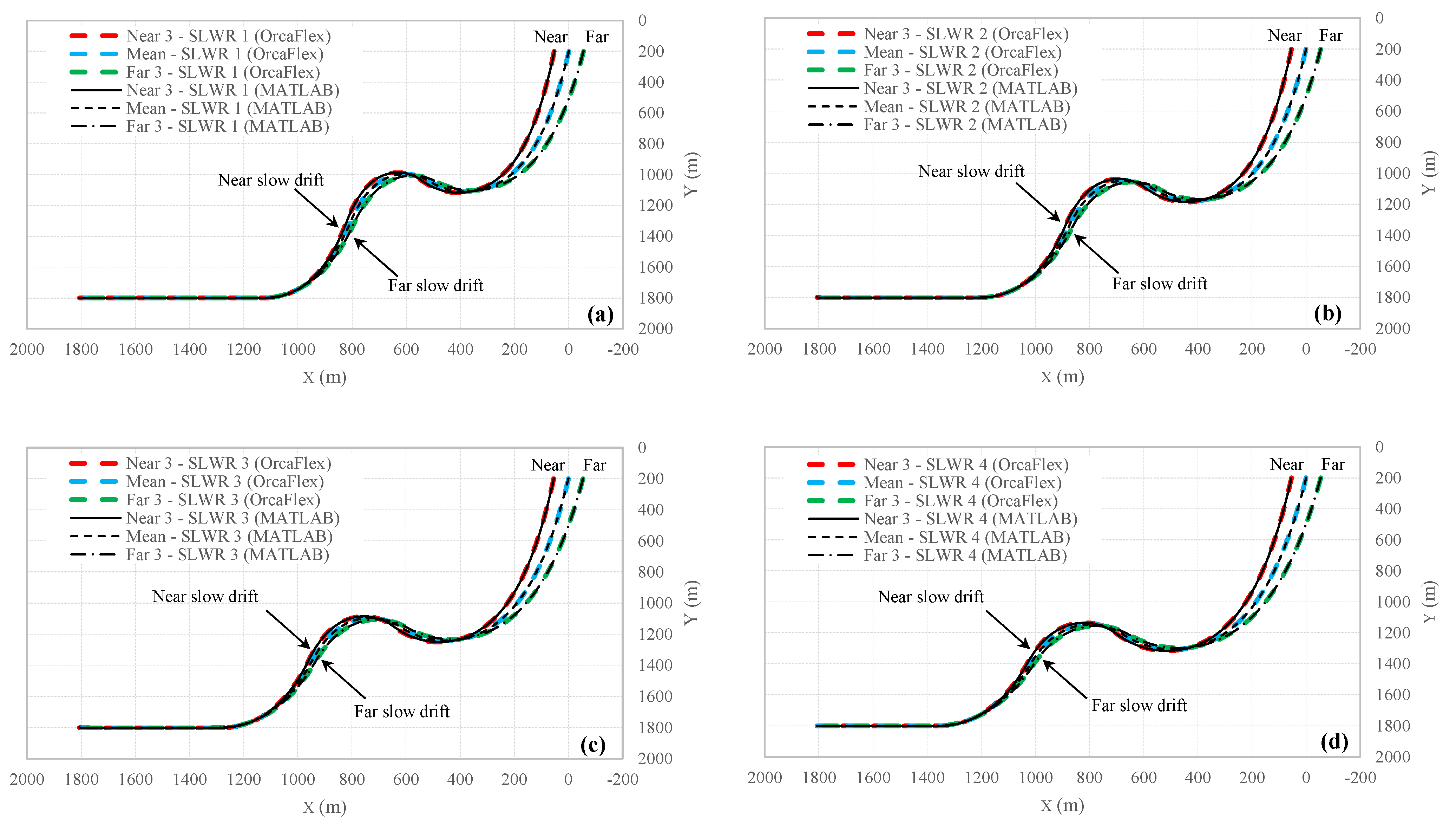
3.2. Riser Data and Verification of Analytical Responses

This section presents the data utilized for the analytical study of steel lazy-wave risers (SLWRs). Detailed tables, including the mechanical properties of the riser, buoyancy module specification and locations, hydrodynamic coefficients, and seabed characteristics, serve as the foundational input for the analysis. The comprehensive riser data are fed into a MATLAB algorithm to simulate the riser’s behavior under a range of operational conditions. To ensure the accuracy and reliability of the analytical responses, the results obtained from the MATLAB algorithm are rigorously compared against those from established numerical simulation software such as OrcaFlex under both mean and extreme boundaries for vessel positions in near and far directions. This comparative analysis evaluates the riser’s configuration and internal forces, ensuring that the MATLAB-generated results align with the expected physical behavior of SLWRs. The successful verification of the analytical responses highlights the effectiveness of the MATLAB algorithm in accurately predicting the performance of SLWRs. This crucial step provides a solid foundation for a reliable discussion on the behavior of SLWRs in the parametric study section.

• SLWR data used in analysis

Table 1. SLWR parameters for the case study.

Parameter	Value
Outer diameter	0.324 m
Thickness	0.0205 m
Riser length	3000 m
Water depth	1800 m
SLWR top height from seabed	1600 m
Bending stiffness	4.67 × 107 N.m2
Soil stiffness	5.91 kN/m/m

represents the key data for analytical and numerical studies.

The following part represents the view of the general result of SLWRs with different buoyancy modules (

Table 2. Hang-off angle of SLWRs in mean locations.

Type	${\mathit{\theta }}_{0,\mathit{m}\mathit{e}\mathit{a}\mathit{n}} \left(\mathbf{d}\mathbf{e}\mathbf{g}\right)$	${\mathit{S}}_1 \left(\mathbf{m}\right)$	${\mathit{S}}_2 \left(\mathbf{m}\right)$	$\mathbf{Total} \mathbf{Length} \left(\mathbf{m}\right)$
SLWR 1	82.433	1200	500	3000
SLWR 2	82.263	1300	500	3000
SLWR 3	82.066	1400	500	3000
SLWR 4	81.842	1500	500	3000

).

• SLWR results in mean position

The mean position hang-off coordinates are set at ($X=0,Y=0$), while the displaced hang-off coordinates are positioned at 3% of the water depth on both sides of the mean position. Every station of the vessel has 1% water depth relocation compared to its neighbor and includes three stations in the near and three stations in the far zone. Figure 7 presents a view of the configuration of different risers (based on different positioning of the buoyancy module) and stations for the riser’s top node positions.

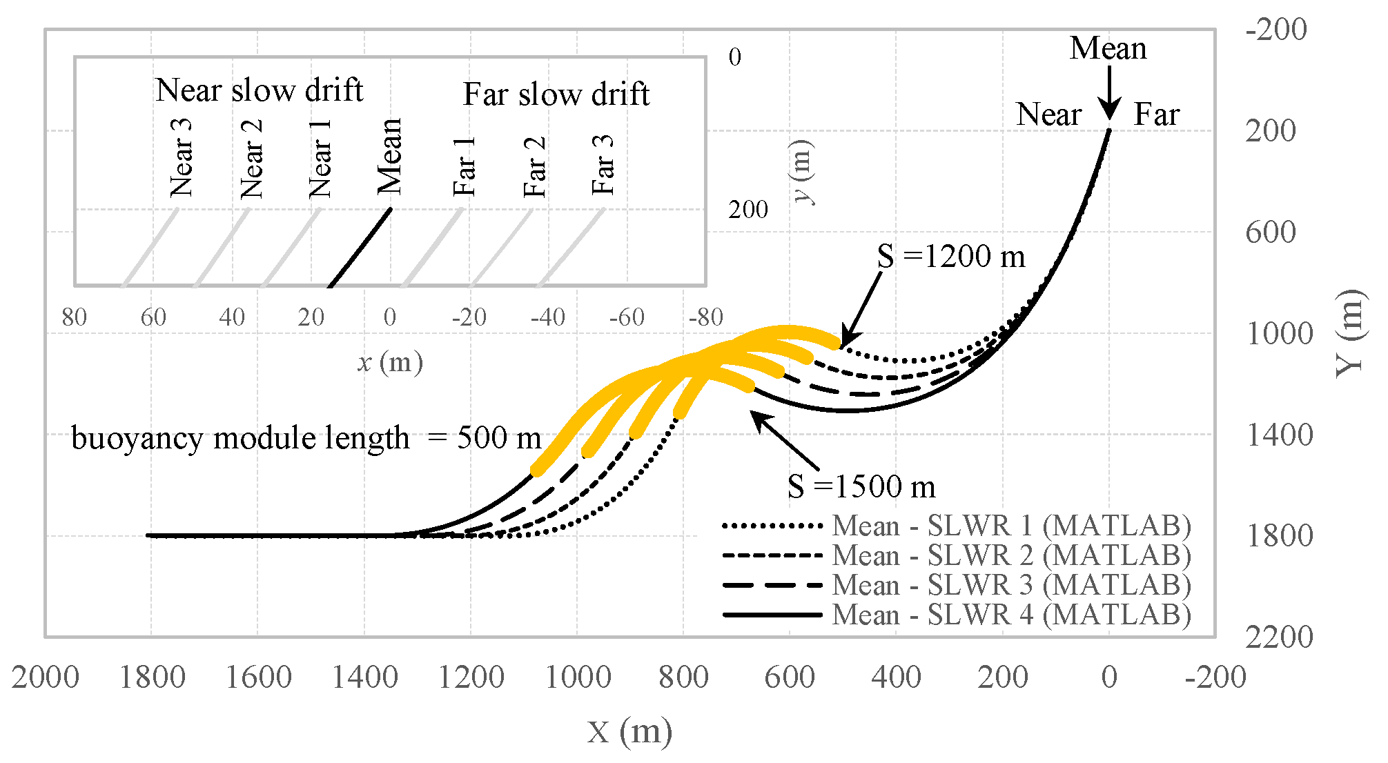
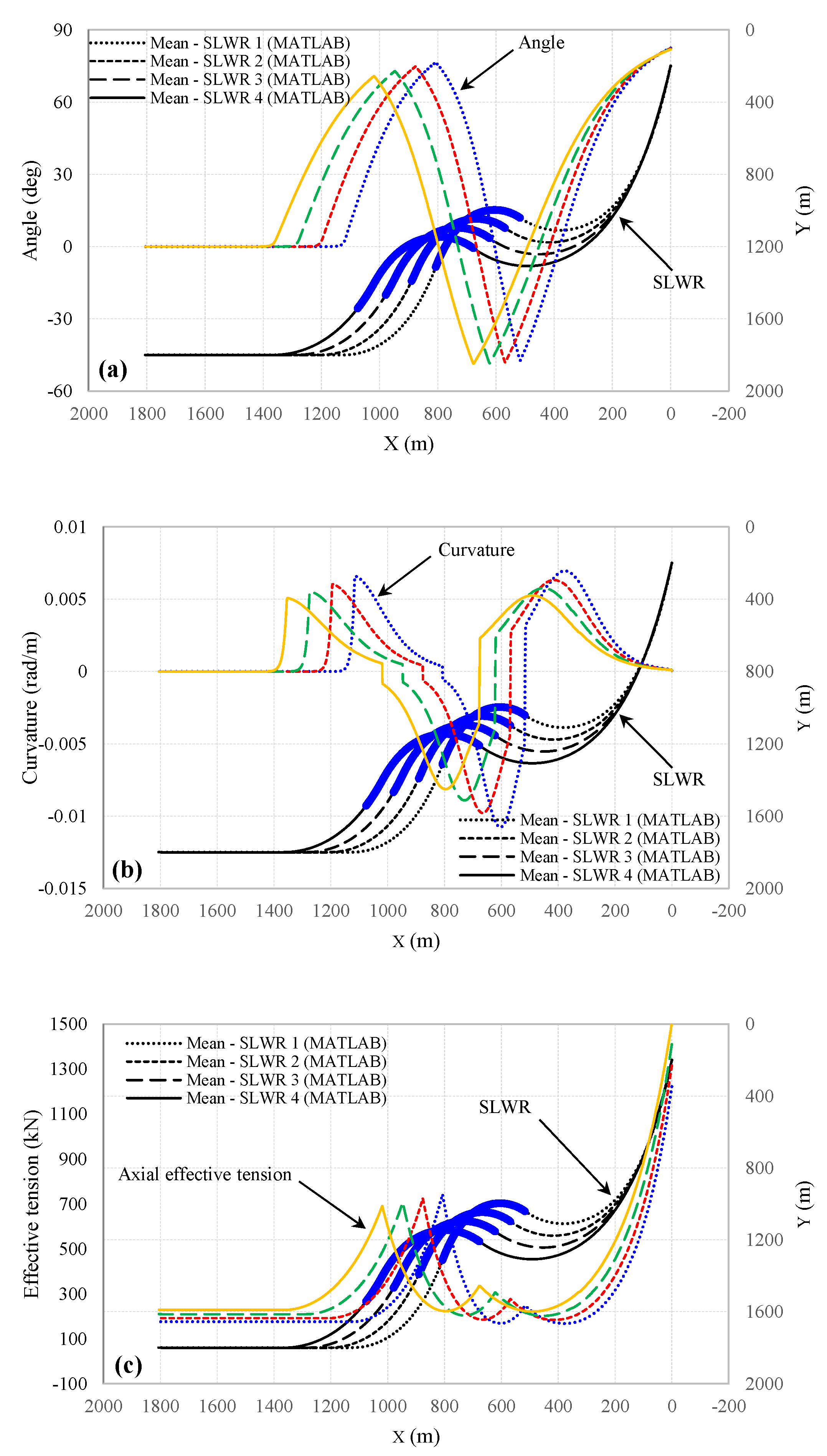
A standard steel lazy-wave riser is selected and deployed at a water depth of 1800 m, featuring an equilibrium hang-off inclination angle, as mentioned in Table 2. Figure 8 illustrates the comparison between the configurations of various lazy-wave risers, including the slope and curvature along the riser. In all cases, the same buoyancy module is considered, with detailed specifications provided in

Table 3. Buoyancy module geometry.

Parameter	Value
Outer diameter	0.8 m
Thickness	0.324 m
Bending stiffness	4.67 × 107 N.m2

,

Table 4. Different densities in the material.

Material	Density kg.m3
Riser	7850
Hydrocarbon	800
Buoyancy module	500
Water	1025

and

Table 5. Hydrodynamic coefficients [14].

Element	Drag Coefficient
	$\mathbf{Normal} ({\mathit{C}}_{\mathit{d}}$)	$\mathbf{Tan}\mathbf{gential} ({\mathit{C}}_{\mathit{\tau }}$)
Riser	1.2	0.036
Buoyancy module	1.07	0.166
The current velocity is 0.2 (m/s).

.

Changes in the slope and curvature resulting from the placement of buoyancy modules at greater depths provide a lower gradient for the riser near the TDP (SLWR 4). This phenomenon can explain why deeper buoyancy module placement yields better stress variation results (which will be discussed later), compared to higher placement with a shorter $S_1$.

Implicitly, it can be concluded that using a buoyancy module at greater depths (SLWR 4) creates a smaller boundary layer due to the reduced curvature gradient at the TDP compared to modules placed at the top of the riser (SLWR 1). This conclusion is further supported by Figure 8c, which shows that the axial force is higher in the touchdown segment and the TDP for the fourth module. Thus, a smaller boundary layer length is needed.

• Verification of analytical responses

Figure 9, Figure 10, Figure 11, Figure 12, Figure 13, Figure 14 and Figure 15 illustrate the comparison between the mathematical and numerical results of the configuration, curvature, effective tension, wall tension, direct tensile stress, maximum cross-sectional bending stress, and total axial stress along the steel lazy-wave riser when exposed to vessel slow drift motion and ocean current for different types of SLWRs on the nearest, mean, and the farthest positions of the vessel. To improve clarity, the representations of SLWR performance within the TDZ under equilibrium conditions are displayed at an enlarged scale in each figure. Upon careful examination of these figures, it becomes evident that the outcomes obtained from both approaches exhibit a high degree of concurrence.

Figure 10 illustrates the curvature of the riser. The figures demonstrate that the maximum curvature occurs at three locations: two in the suspended section and one at the TDP, indicating that the riser exhibits three peaks. Additionally, it is observed that in all types of risers, regardless of the buoyancy module placement, the maximum curvature occurs when the vessel is in the near position. Among the different riser types, the first type exhibits the highest curvature values at the peaks, while the fourth type shows the lowest curvature values. This implies that increasing the distance $S_1$ mitigates the curvature values and, consequently, the bending moments.

The following section presents the results for effective stress and wall stress under various conditions for all four types of risers. The results indicate that the maximum axial force occurs at the HOP and decreases towards the TDP, with the minimum value observed at the seabed. The axial force values in the riser at the TDZ show minimal differences among the different riser types, in contrast to the findings reported by Ruan et al. (2019) [14]. This consistency in axial force can be attributed to the reduced amplitude of HOP oscillations and defining the axial tension distribution in the boundary layer, resulting in less variation. Axial tension along the touchdown segment remains consistent due to the disregarded seabed friction in both mathematical and numerical analysis.

The following section illustrates the axial stress resulting from wall tension. The maximum axial stress occurs at the HOP, while the minimum is observed at the seabed. Notably, the axial stress in the riser increases when the vessel is positioned in a far location. Additionally, employing the fourth type of riser leads to reduced axial stress on the riser. This suggests that positioning the buoyancy module closer to the seabed results in a lower axial stress due to wall tension. Also, axial stresses along the touchdown segment remain consistent due to the disregarded seabed friction in both mathematical and numerical analysis.

The following section presents the axial stress magnitude resulting from bending moments along the riser for different riser types at various locations. According to the curvature results, three locations with local maxima for axial stress due to bending are identified. The values of the axial stress magnitude resulting from bending align with the curvature plots. Additionally, a close examination of the TDZ reveals that the maximum axial stress due to bending occurs over a shorter length of the suspended riser when the vessel is in the near position, which is a consequence of the TDP shifting.

The stress variations and fatigue concerning TDP displacement due to vessel movement was extensively analyzed by Shoghi and Shiri (2019) [5]. Their MATLAB calculations for a steel catenary riser (SCR) demonstrated a significant correlation between bending variations and TDP displacement. Their results were limited to vessel displacements of approximately 2% of water depth on either side of the mean position. In their study, the riser contained high axial tension, but its axial tension variations were not substantial. Axial stresses along the touchdown segment remained consistent due to null curvature away from the TDP toward the anchor end.

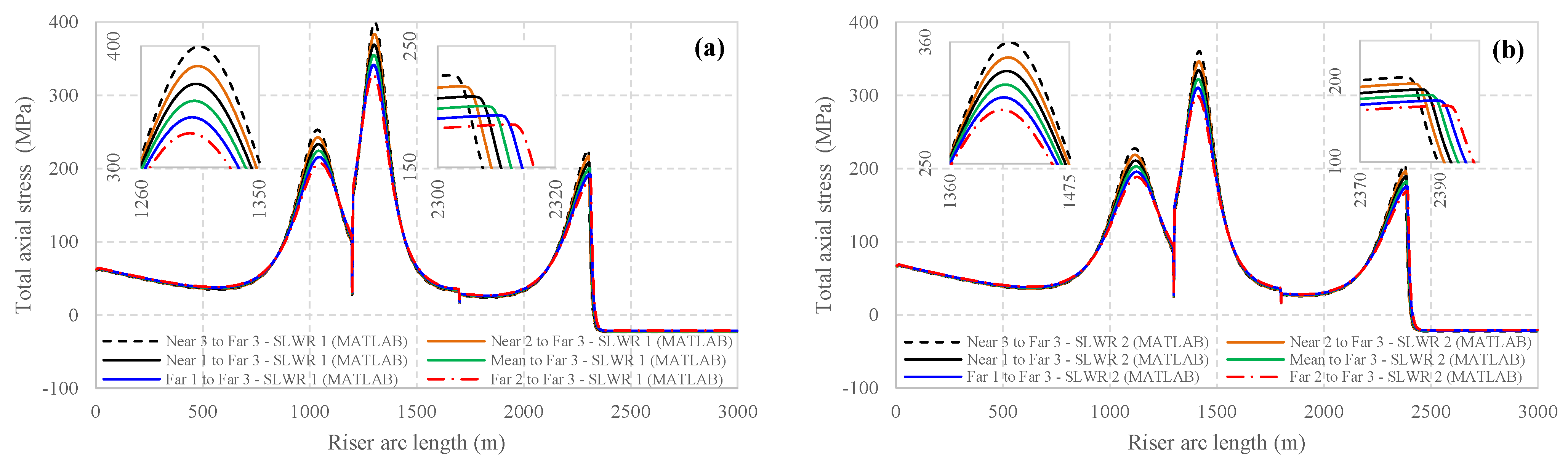
Figure 15 presents the magnitude of total axial stress along the length of various riser types at different locations. According to the curvature and axial tension results, the locations of the maxima for total axial stress tend to behave similarly to the bending distribution. The axial stress values due to bending align with the descriptions provided for the curvature plots. Additionally, a close examination of the TDZ reveals that the maximum axial stress occurs when the vessel is in the near position and when the riser module has a shorter hang-off section.

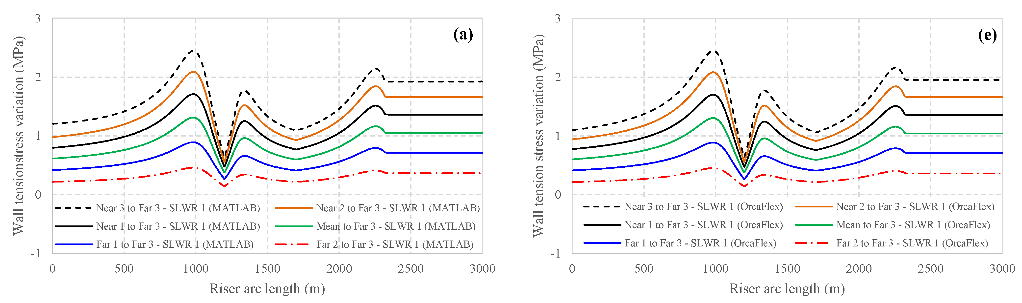
4. Axial Stress Variation: Effect of Vessel Motion and Buoyancy Segment Location

This section presents the variations in axial stress due to axial force, considering a variable axial force in the boundary layer in the analytical model. The analytical model results are compared with those from the numerical model. The figures show excellent agreement, which is particularly valuable when the vessel experiences significant slow drift motion (Figure 16, Figure 17, Figure 18, Figure 19, Figure 20 and Figure 21).

This figure indicates that the highest stress variations due to axial force occur in the sag and TDZ regions. Although effective and wall tension stresses reach their minimum values in the TDZ, local maximum axial stress variations still occur.

The results demonstrate a strong correlation between axial stress variations and vessel slow drift motion. The maximum stress variations are observed for the largest displacements relative to Far 3, particularly when the vessel is positioned in Near 3. Previous results indicated that the axial force in the fourth riser was highest at the TDP, resulting in less curvature at the TDP. However, this can be generalized to axial force variations.

Given that the authors have calculated the tension distribution within the boundary layer, analytical results based on these calculations are utilized. This approach contrasts with the methodology employed by Ruan et al. (2019) [14], who used OrcaFlex software results to account for axial stress variations due to tension in the riser in their model. In quasi-static calculations for axial stress variations, the stress difference at each node on the riser is computed relative to the vessel’s position at Far 3.

To investigate the effect of buoyancy module placement, the stress variations for each riser type are plotted and validated against similar results obtained from OrcaFlex (see Figure 17). The OrcaFlex model uses the finite elements based on the line theory. The riser is discretized by five-meter-long elements in the catenary section and one-meter-long elements in the TDZ for more accurate results of seabed interaction. The riser–seabed interaction is incorporated by using the built-in non-linear hysteretic model proposed by Randolph and Quiggin (2009) [27]. Inextensibility of the riser in OrcaFlex is enforced by considering the axial stiffness as one hundred times the value of the real riser’s. The inextensibility of the riser is not expected to remarkably affect the axial tension in the TDZ. However, for extreme environmental loads, the inextensible riser may experience high-frequency oscillations within the early wave periods that need to be supervised in structural analysis. The findings indicate that for a constant vessel excitation, the deeper the buoyancy module is installed (the greater the distance from the HOP), the greater the axial stress variations. SLWR 4 produces a high-tension and high-stress variation.

Figure 18 illustrates the variations in axial stress due to bending moments on the riser. The stress variation curve exhibits four peaks: Two are located at the points of maximum bending in the suspended section, and two are at the points of maximum bending in the TDZ. The magnitudes of axial stress variation correlate with the amplitude of vessel relocation.

Additionally, the results show that for the same vessel excitation, deploying the buoyancy module at greater depths (SLWR 4) is more effective in reducing axial stress variations, thereby increasing fatigue life compared to placing the buoyancy module at higher levels. However, previous results indicated that increasing the depth of the buoyancy module had the opposite effect on axial stress variations due to axial force.

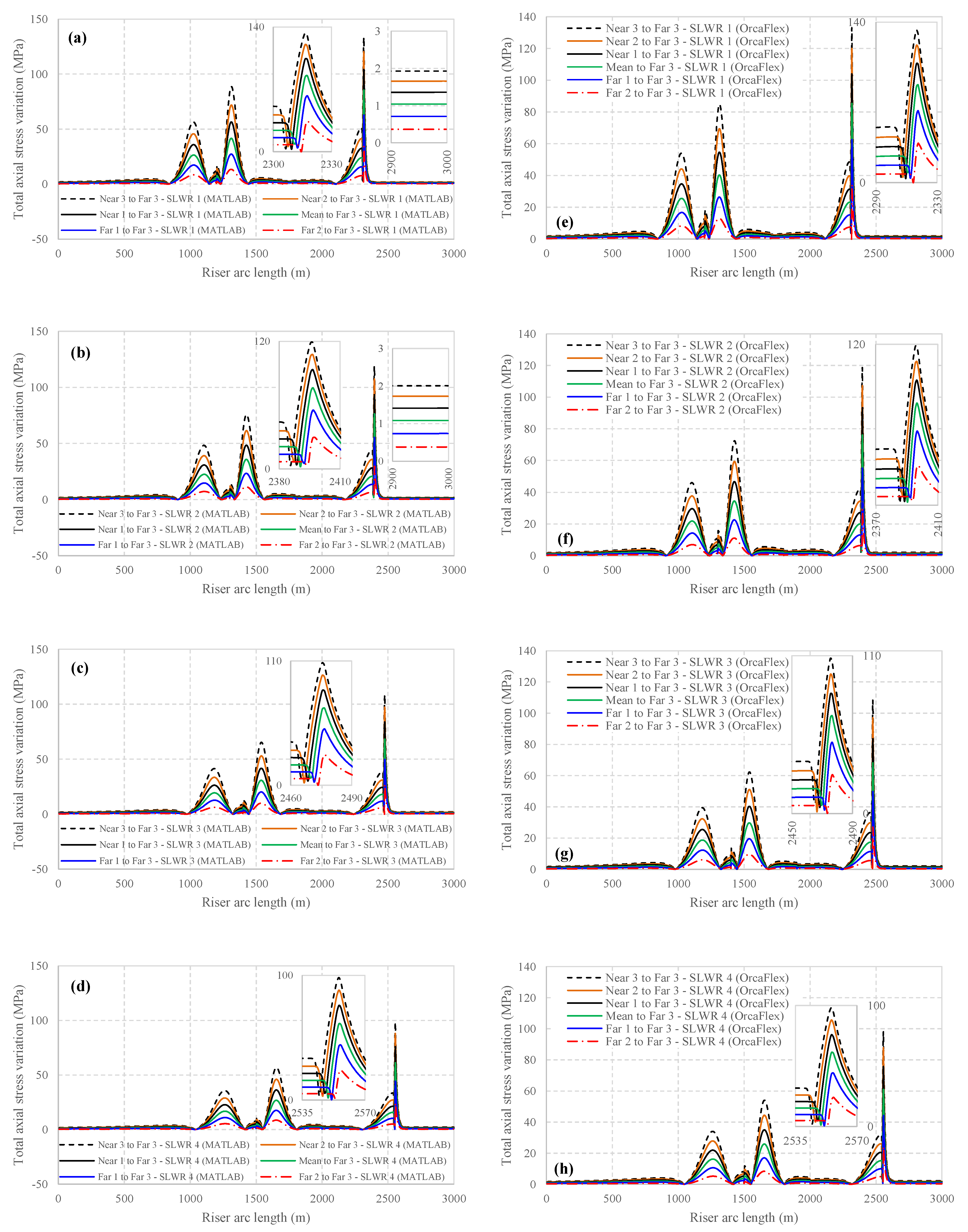
Figure 19 represents the total axial stress variation on the riser in the different mentioned situations. The results indicate that the primary source of stress variation is the bending variation. The graph shows four peaks: two occurring at the points of maximum bending in the suspended section and two at the points of maximum bending in the TDZ. In all these peaks, the fluctuations in axial stress resulting from bending exhibit a significant correlation with the vessel’s displacement. Furthermore, the results demonstrate that for the same vessel excitation, placing the buoyancy module at greater depths (SLWR 4) is more effective in reducing axial stress variations due to bending, thus enhancing fatigue life compared to positioning the buoyancy module at higher levels.

However, previous results, as shown in Figure 16, indicated that increasing the depth of the buoyancy module has the opposite effect on axial stress variations due to axial force. This contrast highlights the complex interplay between different types of stress variations and the importance of optimizing buoyancy module placement for overall riser performance.

Figure 20 illustrates the total axial stress variations at four different stations relative to the vessel’s position at Far 3 for various SLWR types. As the vessel moves farther from the Far 3 station, the total stress variations increase.

The outputs indicate that the stress variation values in the riser depend not only on the vessel’s position but also on the buoyancy module placement. Specifically, when the vessel is positioned at the same relative location as Far 3, the stress variations are lower for deeper buoyancy module placements (SLWR 4). Reduced excitation amplitude in the vessel and a longer hang-off section are two key factors that contribute to the decreased stress variation amplitude, ultimately leading to reduced fatigue failure.

Figure 21 illustrates the variations in axial stress due to bending, which has been previously identified as the primary source of fatigue failure, for various types of SLWRs compared to the equivalent SCRs (with the buoyancy module removed) between two vessel positions. The figure suggests that there is a minimum length for the hang-off section (for a given $S1$) beyond which placing the buoyancy module increases the fatigue life of the SLWR compared to the SCR.

The results indicate that the use of a buoyancy module does not necessarily lead to increased fatigue life (Figure 21). Employing SLWRs instead of SCRs with an appropriately positioned buoyancy module reduces the total axial stress variations that cause fatigue in the riser. It is important to note that decreasing the distance between the buoyancy module and the vessel (reducing $S1$) increases the total axial stress variations, potentially exceeding those in the SCR configuration.

5. Conclusions

This research aimed to provide a precise estimation of the static axial stress range for deepwater steel lazy-wave risers (SLWRs) subjected to ocean currents under operational conditions. By applying the natural catenary theory for risers far from the touchdown zone (TDZ) and the linear deformation theory of beams for the TDZ, this study examines the deformation, internal forces, and axial stress distribution across an SLWR cross-section. In this framework, the authors utilized a boundary-layer method, previously developed to study riser–seabed interactions near the touchdown point, and extended its application to boundary layer zones. Meticulous consideration of axial tension within this zone analytically showed a high degree of concordance in the axial stress variations in the TDZ resulting from axial force. A comprehensive study on the structural response of SLWRs, considering vessel drift motion and different buoyancy module locations, was conducted, with results compared to those obtained via commercial software, OrcaFlex.

As a result of the vessel’s slow drift motion, four distinct peaks in the axial stress range are observed along the SLWR’s arc length: two in the sag and hog zones, and two in the TDZ. Axial stress fluctuations from the hang-off point to the TDZ of the SLWR are primarily dominated by variations in bending stress. In contrast, stress variations on the touchdown segment far from the TDP are predominantly influenced by axial force. Notably, smaller vessel slow drift motions result in minimal stress variations.

The results demonstrate that, for the same vessel excitation, placing the buoyancy module at greater depths (SLWR 4) is more effective in reducing axial stress variations due to bending, thus enhancing fatigue life compared to positioning the buoyancy module at near-to-hang-off-point levels. However, increasing the buoyancy module depth has the opposite effect on axial stress variations due to axial force. This contrast highlights the complex interplay between different types of stress variations and underscores the importance of optimizing buoyancy module placement for overall riser performance.

As the amplitude of the vessel’s slow drift increases, the maximum axial stress ranges also increase. The findings of this research suggest that while SLWRs are typically used instead of steel catenary risers (SCRs) to mitigate stress variation in the TDZ, employing SLWRs with buoyancy modules can also worsen stress variation if not appropriately positioned. Therefore, it is prudent to position the buoyancy segment closer to the seabed while ensuring the integrity of the lazy-wave configuration.