Article

Time Prediction in Ship Block Manufacturing Based on Transfer Learning

1
College of Mechanical and Electrical Engineering, Harbin Engineering University, Harbin 150001, China
2
Sanya Nanhai Innovation and Development Base of Harbin Engineering University, Harbin Engineering University, Sanya 572024, China
3
College of Shipbuilding Engineering, Harbin Engineering University, Harbin 150001, China
4
Shanghai Waigaoqiao Shipbuilding Co., Ltd., Shanghai 200137, China
*
Authors to whom correspondence should be addressed.
J. Mar. Sci. Eng. 2024, 12(11), 1977; https://doi.org/10.3390/jmse12111977
Submission received: 24 August 2024 / Revised: 28 October 2024 / Accepted: 31 October 2024 / Published: 2 November 2024
(This article belongs to the Section Ocean Engineering)

Abstract

:
Accurate time prediction is critical to the success of ship block manufacturing. However, the emergence of new ship types with limited historical data poses challenges to existing prediction methods. In response, this paper proposes a novel framework for ship block manufacturing time prediction, integrating clustering and the transfer learning algorithm. Firstly, the concept of distributed centroids was innovatively adopted to achieve the clustering of categorical attribute features. Secondly, abundant historical data from other types of blocks (source domain) were incorporated into the neural network model to explore the effects of block features on manufacturing time, and the model was further transferred to blocks with limited data (target domain). Leveraging the similarities and differences between source and target domain blocks, actions involving freezing and fine-tuning parameters were adopted for the predictive model development. Despite a small sample size of only 80, our proposed block time prediction method achieves an impressive mean absolute percentage error (MAPE) of 8.62%. In contrast, the MAPE for the predictive model without a transfer learning algorithm is notably higher at 14.97%. Experimental validation demonstrates the superior performance of our approach compared to alternative methods in scenarios with small sample datasets. This research addresses a critical gap in ship block manufacturing time prediction.

1. Introduction

In the shipbuilding industry, the ship is typically divided into several blocks, each constructed separately and gradually assembled. The rational and precise estimation of block construction time is crucial due to its significant impact on the allocation of key resources in shipyards and material procurement. However, the shipbuilding industry exhibits distinct characteristics compared to other manufacturing sectors, such as automobile and aircraft manufacturing. Ships are categorized as single products produced on order, characterized by strong customization, substantial investments, extensive construction workloads, and dense assembly components. These characteristics pose significant challenges for estimating block construction times for ships, especially during shipyard transitions to new vessel types. For instance, a Chinese shipyard has primarily focused on manufacturing container ships and bulk carriers for many years. However, it has gradually begun undertaking orders for high-tech vessel types like cruise ships to meet the demands of expanding business. The inherent differences in block types among various vessels exacerbate the difficulty in predicting block construction times, particularly in the absence of accumulated historical data for new vessel types.
The manufacturing processes for blocks of different ship types are essentially the same. Block manufacturing operations are typically divided into three consecutive construction stages: sub-assembly, unit assembly, and final assembly [1]. The first stage, sub-assembly, involves assembling longitudinal components or reinforcements welded onto the bottom plate to form sub-assembly blocks. In the unit assembly stage, related sub-assembly blocks are assembled to create unit assembly blocks, which are then integrated in the final assembly stage. During the sub-assembly stage, blocks typically have relatively simple geometric shapes, with complexity increasing as construction progresses. Currently, most shipyards utilize a combination of assembly lines and robots for sub-assembly and unit assembly. However, the final assembly stage heavily relies on manual labor due to limited workspace and the complexity of processes. Therefore, this paper focuses on predicting the time of the final assembly stage in block manufacturing.
The accurate prediction of project task durations is crucial for efficient scheduling, budgeting, resource allocation, and overall construction management. Therefore, the estimation of project task durations has always been a focus of researchers’ attention. Considering that project tasks consist of multiple processes, some scholars have approached the problem of estimating project task durations from the processes. You-Ling et al. [2] addressed the uncertainty of working hours in a large-scale customized environment by using group decision theory to construct a model for solving process difficulty coefficients. They employed the analytic hierarchy process to establish an evaluation index matrix and determined the relationship function between process difficulty coefficients and project task durations based on curve fitting. However, their study tasks were relatively simple. Kim et al. [3] decomposed project tasks using the Work Breakdown Structure technique and designed key process duration estimation rules based on the average method, equivalent day work method, and percentage method for different processes. A manufacturing duration estimation model was established; however, the project task durations calculated by this method were relatively rough. Choi et al. [4] analyzed the business processes of ship assembly and developed process quantification formulas of the required operating time based on the characteristics of each process. Finally, they calculated the duration of ship manufacturing tasks through summation. However, the calculation method proposed cannot be directly applied to actual production guidance in shipyards and requires further customization based on the actual environment of shipyards. Prediction methods for project task durations that rely on statistical models and calculation rules often fail to accurately estimate the preparation time between two processes, even though these processes may follow certain patterns. Additionally, these methods require extensive historical data to uncover the calculation rules for each operation process. Undoubtedly, achieving accurate predictions using this approach is challenging, especially when dealing with small sample datasets.
In recent years, data-driven methods have been successfully applied in various fields such as process parameter optimization [5], mechanical fault diagnosis [6], and material performance prediction [7]. These methods utilize complex associative rules among multidimensional feature variables to optimize objectives without needing to elucidate the underlying collaborative mechanisms. So far, in the field of time prediction, regression analysis and neural networks have been very popular. Rizaee and Lei [8] proposed a classification linear regression model for predicting the time of scaffolding construction tasks within the construction industry. They established standardized regression model scoring rules, enhancing the reliability of scaffolding activity task time prediction. Chang et al. [9] developed a prediction model based on backpropagation neural networks (BPNNs) to address the challenge of accurately predicting maximum completion times. They dynamically improved the weight values and threshold values of the model using a self-adaptive immune genetic algorithm. Kong and Li [10] introduced a method that integrates an adaptive time-series feature window with stacked bidirectional long short-term memory networks to forecast the tool remaining useful life in situations where failure data are unavailable. Chen and Wang [11] utilized K-means clustering to categorize simulation tasks in cloud manufacturing and applied artificial neural network (ANN) models to predict task times for each categorized task. Meanwhile, Chen [12] integrated clustering and BPNN models to develop a time prediction model for semiconductor manufacturing tasks. In the shipbuilding domain, Jeong, J. H et al. [13] employed a machine learning approach to predict lead times in shipbuilding processes of the cutting process, block erection, and spool supply chain. This methodology aims to enhance master data management for production lead times, addressing the limitations of traditional engineering methods. Qu and Jiang [14] employed a BPNN model to forecast the real assembly duration of ship block assembly processes. The model was trained with block weight, block type, number of assemblies, and assembly length as inputs, while assembly hours served as outputs. Nevertheless, they did not address the utilization of distinct BPNN models to predict assembly hours for blocks exhibiting significant differences. Zhu and Woo [15] proposed a new self-organizing hierarchical particle swarm algorithm with the jumping-time-varying acceleration coefficient–support vector machine regression model to enhance the prediction accuracy of durations in shipbuilding. By leveraging the global search capability algorithm, they optimized support vector machine parameters to improve prediction precision. Li et al. [16] introduced a three-stage approach for predicting block construction time. Initially, the K-means algorithm was utilized to cluster ship blocks. Subsequently, an improved slack-based measurement model was applied to reveal the regularity of effective time allocation assessment for each block. In the final stage, knowledge about block characteristics and efficient time allocation for block construction activities was acquired through BPNN models. However, the premise of studies in the literature assumes that shipyards have access to a significant amount of historical data in the operational domain, which does not address the challenge of task time prediction with small sample datasets.
Predicting targets in small sample datasets is a pressing issue addressed in this paper. Liu and Dai [17] tackled the phenomenon of overfitting and the poor generalization performance of product quality prediction methods in small-sample, high-dimensional-data environments by proposing a combined method of data augmentation and model optimization. Kang et al. [18] proposed a virtual sample generation method based on overall trend differential evolution to accurately predict the remaining life of lithium batteries in small sample datasets. Li et al. [19] proposed a method of employing virtual samples to build early high-dimensional manufacturing models, which systematically adds artificial samples to fill the data gaps. In their study, a small dataset learning task in the array process of a thin-film transistor liquid-crystal display panel manufacturer was addressed using only 20 samples to learn the relationship between 15 inputs and 36 output attributes. Li et al. [20] proposed the attribute-trend-similarity method to improve learning performance for small datasets. This method considers the relationships among attributes in the value generation procedure and uses a non-parametric process to learn trend similarities among attributes. It then estimates the corresponding ranges of attribute values based on these trends when other attribute values are given. El Bilali et al. [21] overcame the limitations of small sample datasets by integrating adaptive algorithms into data augmentation methods to predict health risks related to coliforms in drinking water. Additionally, the application of transfer learning to the problem of small sample datasets has received significant attention from scholars. The essence of transfer learning is to learn knowledge from the source domain and transfer it to another different but similar target domain to reduce the reliance on target domain data [22]. Currently, transfer learning is widely studied in fields such as text classification [23,24], computer vision [25], and natural language processing [26]. Due to the difficulty in collecting sufficient historical data in many practical industries, scholars have combined transfer learning with data-driven methods in areas such as mechanical fault detection [27,28], fault diagnosis [29,30], and remaining useful life prediction [31,32]. Hung and Gan [33] proposed a method that learns and transfers knowledge from large data samples to reduce the search space of small sample data by employing transfer learning. Zhao [34] proposed a deep convolutional neural network (CNN) model based on transfer learning to address the issue of overfitting in small sample datasets during image recognition, thereby enhancing the classification recognition rate of image processing. Chen et al. [35] developed a long short-term memory neural network (LSTM) model based on transfer learning to address the aging issue of lithium-ion batteries. The model utilized experimental battery aging data as the source domain and automotive battery aging data as the target domain to achieve aging state prediction for target batteries. Li et al. [36] addressed the challenge of limited data in early warning systems for tunnel excavation collapse in new tunneling projects. They utilized historical tunneling data to forecast the real-time excavation status of new tunnel projects through transfer learning. Li et al. [37] considered the high cost and long cycle of gear contact fatigue tests and proposed a prediction method based on BPNN and transfer learning. Based on the analysis of the literature, transfer learning is an effective approach to handle small sample datasets.
Despite the considerable body of research on predictive modeling for ship block manufacturing, existing methods in shipyards show notable shortcomings in accurately predicting manufacturing times. This gap highlights the need for innovative approaches, particularly those leveraging promising machine learning techniques. However, the effectiveness of machine learning methods is often limited by the challenges presented by small sample datasets. Therefore, it is imperative to develop a robust ship block manufacturing time prediction framework tailored for small sample datasets and ship block manufacturing features, and to validate its effectiveness using real shipbuilding data. This study is of extraordinary significance, as it seeks to bridge the gap between existing methodologies and the unique challenges posed by ship block manufacturing.
Therefore, this paper proposes a ship block manufacturing time prediction framework based on the combination of clustering and transfer learning to achieve ship block manufacturing time prediction for small sample historical datasets. In this framework, blocks with abundant historical data are considered as the source domain, while the blocks to be predicted in the small sample dataset are considered as the target domain. Firstly, the source domain blocks are clustered based on their structural characteristics, and the target domain blocks are mapped to the clustering clusters. Secondly, neural network models are trained separately for each cluster formed by clustering the source domain blocks, discovering the knowledge of the potential impact of features on block manufacturing time. Then, the pertinent model acquired from the source domain is transferred to the target domain, and parameters of the model for the target domain blocks are frozen and fine-tuned based on the similarities and differences in features between the source and target domain blocks. This paper facilitates the precise prediction of ship block manufacturing time with small sample datasets.
The remainder of this paper is organized as follows. Section 2 presents a description of the proposed method. Experimental evaluations are reported in Section 3. Discussion is provided in Section 4. Conclusions and suggestions for future research are presented in Section 5.

2. Proposed Method

The paper aims to discover knowledge related to the assessment of target ship block manufacturing time and to achieve predictions in small sample datasets. This paper presents a two-stage method, the framework of which is illustrated in Figure 1. The detailed stages are outlined as follows:
Clustering: In manufacturing, product characteristics play a pivotal role in production activities [38]. Ship blocks with varying characteristics demonstrate considerable differences in manufacturing time. For instance, blocks of equal weight may necessitate varying manufacturing times depending on factors such as block shape, number of unit assembly blocks involved, and process types. However, with the increasing standardization of block manufacturing processes, blocks with similar structures often exhibit comparable operational time patterns. Therefore, this paper aims to cluster the target domain blocks of small sample datasets. However, existing clustering methods frequently encounter limitations in effectively clustering small sample datasets [39]. Given the similarities in manufacturing processes, block type division, and welding processes between target domain blocks and source domain blocks, this paper adopts a research approach that involves clustering the source domain blocks and mapping the target domain blocks to achieve clustering of the target domain blocks clusters.
Training: A significant body of research suggests that neural network models optimized using particle swarm optimization algorithms (PSO-BPNN) outperform basic neural network models [15,40,41]. Moreover, the prediction accuracy of BPNNs correlates closely with the available sample size [37]. Therefore, this paper proposes the neural network models optimized using particle swarm optimization algorithms and the transfer learning (TR-PSO-BPNN) model involving three actions: transfer, freeze, and fine-tune. Initially, the PSO-BPNN models are initially trained on the clustered source domain blocks. Subsequently, the trained parameters of the model are transferred to the TR-PSO-BPNN models of the target domain blocks. Leveraging the similarities and differences between source and target domain blocks, actions involving freezing and fine-tuning neural network model parameters are adopted to train the TR-PSO-BPNN model on the clustered target domain block data. The outcome of this stage is the development of the TR-PSO-BPNN model capable of predicting the manufacturing time of target domain blocks.

2.1. Operational Process Description

To predict the time required for the final assembly stage of ship block manufacturing, it is essential to delineate the operational processes and characteristics pertinent to this stage. The final assembly stage can be defined as the procedure involving the assembly of unit assembly blocks in accordance with the process route map through manual interactions [4]. The detailed assembly process of the final assembly stage primarily encompasses positioning, spot welding, flipping, welding, and grinding. Positioning operation involves relocating the requisite unit assembly blocks to the designated joint line position. During this process, fixtures are utilized to secure the unit assembly blocks, while cranes are employed to elevate them to the desired position. Spot welding is employed to affix objects using localized welding techniques, ensuring the stability of unit assembly blocks in their positioned state prior to the welding process. The flipping process entails maneuvering the unit’s assembly when operations on their rear surfaces are necessitated. Welding involves the bonding of solid materials together through the application of heat and pressure, which constitutes a significant portion of the working time in the ship block manufacturing process. Grinding encompasses the post-welding operation of welding seams to achieve surface refinement. Typically, the extent of grinding is proportional to the length of the welding seam.

2.2. Data Preprocessing

In the context of block manufacturing, during the process of block clustering and neural network model development, the original sample feature data often exhibit varying scales. To ensure uniformity across all numerical feature data, this paper employs decimal scaling to normalize the feature data. The specific calculation methods are shown in Equations (1) and (2).
y i f = x i f / 1 0 k j
k j = log 10 ( max ( x i f ) )
where y j f represents the normalized feature data and x i f represents the original value of the feature data.

2.3. Block Clustering to Partition the Data Space

2.3.1. Define Features for Clustering

Clustering is crucial in data mining as it entails grouping items based on their similarities [42]. By identifying patterns within these groups, clustering effectively narrows down the problem space. When predicting ship block manufacturing time, training separate predictive models for each group’s manufacturing times can lead to more accurate results.
Before proceeding with clustering activities, it is essential to determine the input features for clustering. The literature suggests that a limited number of parameters can effectively capture the essential characteristics of activities [43]. The primary factors influencing the manufacturing efficiency of ship blocks include block weight, projected area, number of unit assembly blocks, and block type [14,44], which impact the efficiency of operations such as positioning, spot welding, and flipping. Moreover, research indicates that the types of slopes and welding seam significantly affect welding speed [45]. Therefore, this paper selects the six types of block features as candidates for clustering. Detailed information about these features is shown in Table 1.

2.3.2. Block Clustering

Considering that block clustering does not strictly adhere to a binary membership relationship, this paper requires the adoption of a soft clustering method to achieve ship block clustering. Fuzzy C-means clustering, based on fuzzy set theory, extends membership to arbitrary values between 0 and 1. The closer a value is to a cluster center, the higher the similarity between them [46]. However, basic fuzzy C-means clustering is more suitable for clustering numerical attribute features. In contrast, ship block clustering includes both numerical and categorical mixed classification attribute features, and some categorical attribute features exhibit distributed characteristics. For instance, a block may simultaneously have type I and type V slopes. Therefore, this paper innovatively adopts the concept of distributed centroids to achieve clustering of categorical attribute features. Initially, an improved fuzzy C-means clustering is applied to the source domain blocks to generate clustering information. Then, target domain blocks are mapped to the source domain set. Lastly, clustering clusters for both source and target domain blocks are formed.
Let X = { X 1 , X 2 , , X n } denote a set of n data blocks to be clustered and X i ( 1 i n ) be represented by t attributes A 1 , A 2 , , A f , A t . Each attribute A f describes a domain of values denoted by D o m ( A f ) . The attribute domains associated with this paper include numerical and categorical domains. The numerical domain is represented by continuous numerical values, and the categorical domain is represented by finite sets which are usually denoted by D o m ( A f ) = { a f 1 , a f 2 , , a f l , a f s } , where f is the number of category values of the categorical attribute A f . In this paper, since each data block has t attributes, X i can be represented as a vector [ x i 1 , x i 2 , , x i f , , x i t ] . Due to the distributed attribute characteristics of categorical domain features, x i f can be represented as a set { { a f 1 , φ i f 1 } , { a f 2 , φ i f 2 } , , { a f l , φ i f l } , { a f s , φ i f s } } , where φ i f l represents the proportion of occurrences of a f l . Let C = { C 1 , C 2 , , C k , C j , C c } denote a set of c cluster centers, where C j ( 1 j c ) can be represented as a vector [ c j 1 , c j 2 , , c j f , , c j t ] .
The objective function of the improved fuzzy C-means clustering proposed in this paper is shown in Equation (3) and the constraint is shown in Equation (4).
J I F C M = i = 1 n j = 1 c u i j m d ( X i , C j )
s . t . j = 1 c u i j = 1
where u i j represents the degree of membership of X i to the cluster center C j , and m denotes the fuzziness index. d ( X i , C j ) is the dissimilarity measure from data X i to the cluster center C j .
The solution for u i j using the Lagrange multiplier method is shown in Equation (5).
u i j = [ 1 / d ( X i , C j ) ] 1 / m 1 / k = 1 c [ 1 / d ( X i , C k ) ] 1 / m 1
In Equation (5), d ( X i , C j ) is given as follows:
d ( X i , C j ) = f = 1 t d ( x i f , c j f )
where
d ( x i f , c j f ) = ( x i f c j f ) 2     i f   t h e   A f   a t t r i b u t e   i s   t h e   n u m e r i c   a t t r i b u t e μ f δ ( x i f , c j f )     i f   t h e   A f   a t t r i b u t e   i s   t h e   c a t e g o r i c a l   a t t r i b u t e
When the A f attribute is numerical, c j f is shown in Equation (8).
c j f = ( i = 1 n u i j m x i f ) / ( i = 1 n u i j m )
When the A f attribute is categorical, the weight coefficient set for the feature attribute A f is represented by μ f . Based on the distribution centroid, c j f is given as follows.
c j f = { { a f 1 , ω j f 1 } , { a f 2 , ω j f 2 } , { a f l , ω j f l } , { a f s , ω j f s } }
In the above,
ω j f l = i = 1 n η ( x i f )
0 ω j f l 1 ,   1 l s , l = 1 s ω j f l ω j f l = 1 ,   1 f t .
where
η ( x i f ) = u i j / i = 1 n u i j ,   i f   x i f = a f l 0 ,   if   x i f a f l
In Equation (7), δ ( x i f , c j f ) is calculated according to Equations (13) and (14).
δ ( x i f , c j f ) = l = 1 s ϑ ( x i f , a f l )
ϑ ( x i f , a j l ) = max ( 0 , φ i f l ω j f l )
After completing the clustering of the source domain and forming the collection of cluster centers and cluster sets, each block in the target domain is evaluated for its distance to each source domain cluster center using Equation (6). The cluster set corresponding to the minimum distance is deemed the optimal mapping target. Ultimately, this paper facilitates the construction of cluster clusters for the target domain blocks.

2.4. Model Development

2.4.1. Model Prediction Effect Evaluation Indexes

The mean absolute percentage error ( M A P E ) and the coefficient of determination ( R 2 ) are used to evaluate prediction performance. MAPE indicates the average error magnitude of the predictions in this paper. R 2 further elucidates the degree of fit. The specific calculation methods are provided in Equations (15) and (16).
M A P E = 100 % × 1 n i = 1 n ( y i y ^ i ) / y i
R 2 = 1 ( i = 1 n ( y i y ^ i ) 2 ) / ( i = 1 n ( y i y ¯ ) 2 )
where y ^ i is the predicted time of sample X i ; y i is the true time of sample X i ; y ¯ is the mean of y i ; and n is the amount of data in the set.

2.4.2. PSO-BPNN Model of Source Domain Block

To enhance the input data and improve prediction accuracy, this paper further enriches the input feature set based on operational processes and the literature [14,16]. The operational processes involved in the final assembly stage of ship block manufacturing—such as positioning, spot welding, flipping, welding, and grinding—guide the selection of input features for time prediction. Positioning operations, which utilize cranes and fixtures, are influenced by the block’s weight and projected area. The number of unit assembly blocks impacts the overall complexity of the assembly process and, consequently, its duration. Welding, a critical and time-intensive operation, is directly associated with weld seam length and plate thickness, as longer and thicker seams require additional time for heat application and bonding. Finally, grinding, which follows welding, is also contingent upon the length of the weld seam, with longer seams necessitating more extensive finishing work. Therefore, the selected input features—block weight, projected area, number of unit assembly blocks, weld seam length, and plate thickness—are logically derived from the key processes that drive time consumption during the final assembly stage, effectively capturing the essential factors influencing production time. These data are extracted from the design database.
In the PSO-BPNN model, the weights and biases of the model are encoded as particles and updated iteratively using the particle swarm optimization algorithm. It has been proven that a three-layer neural network structure is capable of fitting various nonlinear relationships to meet the required accuracy [47]. Therefore, this paper adopts a three-layer network structure consisting of one input layer, one hidden layer, and one output layer.
After establishing the number of layers in the neural network, the quantity of nodes in each layer is determined. The node count of the input layer is determined by the number of input features, while the node count of the output layer corresponds to the number of prediction indicators. As a result, the PSO-BPNN structure outlined in this paper comprises 5 input nodes and 1 output node. The process of determining the node count of the hidden layer initially involves using an empirical equation (Equation (17)) for initialization and gradually increasing it based on specified rules. The optimal number of nodes in the hidden layer is then determined by calculating M A P E values after executing each neural network model 100 times under varying numbers of hidden layer nodes.
l < n 1                                 l < ( m + n ) + a l = log 2 n                              
where n and m represent the number of neurons in the input and output layers, respectively; l is the number of nodes in the hidden layer; and a is a randomly generated number ranging from 0 to 10. Neural network hyperparameters of the PSO-BPNN model are shown in Table 2.
For the PSO hyperparameters, we selected configurations grounded in prior research on optimal settings [41]. The parameter choices, detailed in Table 3, were set following an extensive review of PSO studies. These hyperparameters are designed to facilitate effective search and convergence properties within the PSO algorithm, supporting robust performance of the PSO-BPNN model in our target prediction task. This systematic approach to hyperparameter selection thus combines empirical testing with insights from the literature, ensuring that the final configurations are both theoretically grounded and empirically validated for our application.

2.4.3. TR-PSO-BPNN Model of Target Domain Block

This paper establishes the TR-PSO-BPNN prediction model for target domain blocks by employing actions such as transfer, freeze, and fine-tuning from the PSO-BPNN model of the source domain. Initially, the PSO-BPNN model of the source domain is transferred to the target domain. Subsequently, considering the primary distinguishing features between the source and target domain blocks, the weights from the input layer to the hidden layer associated with non-primary distinguishing features are frozen to prevent further updates. The remaining parameters in the model are fine-tuned during training on the target domain block data. These actions aim to retain the beneficial impact of similar features between the source and target domain blocks on time prediction while mitigating interference caused by differing features affecting time prediction. The prediction flow chart of the TL-PSO-BPNN model is illustrated in Figure 2.

3. Experimental Evaluation

3.1. Dataset Description

This section provides detailed information about the dataset used in our study, including its origin, feature selection criteria, and sample size.
Data Source: The dataset was collected from a cooperative shipyard in mainland China, which has accumulated extensive data related to ship block manufacturing over time. The shipyard is transitioning to new ship types, such as cruise ships, which has rendered the existing methods for lead-time prediction less effective. To address this, data were extracted from the shipyard’s business database, ensuring the integrity and reliability of the information. Specifically, 1000 bulk carrier blocks were selected as the source domain, and 200 cruise ship blocks were used as the target domain for the experiments.
Feature Selection Criteria: Features were selected based on their relevance to predicting ship block production times. One of the primary distinguishing features between the bulk carrier and cruise ship blocks is the thickness of the steel plates used. Bulk carrier blocks typically have a plate thickness ranging from 12 to 25 mm, while cruise ship blocks generally use thinner plates, with thicknesses ranging from 4 to 8 mm. Other relevant features include block weight, projected area, number of unit assembly blocks, and weld seam length, which were identified as critical factors influencing lead-time prediction.
Sample Size: The dataset consists of a total of 1200 samples, with 1000 bulk carrier blocks serving as the source domain and 200 cruise ship blocks serving as the target domain. These samples represent a diverse range of production scenarios, ensuring a comprehensive evaluation of the model’s effectiveness in different contexts.
All experiments were run on a computer equipped with an Intel Core i7-11390H 3.40 GHz processor manufactured by Santa Clara, located in California, USA, and 16 GB of RAM manufactured by Samsung, located in Seoul, South Korea. Details of the validation are given below.

3.2. Source Domain Block Time Prediction

Utilizing the clustering method proposed in this paper, clustering processing was performed on 1000 source domain blocks. Subsequently, leveraging the formed clustering knowledge, 200 target domain blocks were mapped to the established cluster set. The block clustering results of both the source and target domain are provided in Table 4.
This paper aims to validate the effectiveness of the input features proposed for predicting ship block manufacturing time using the PSO-BPNN model. Furthermore, source domain blocks with and without clustering were compared to demonstrate the advantage of the clustering strategy. A proportion of 70% of the 1000 source domain blocks were allocated for training, and the remaining were utilized for testing. To mitigate the randomness in training, 100 random experiments were conducted. Due to varying sizes in each sample set, the corrected coefficient of determination ( R a d j 2 ) was used to assess R 2 , as shown in Equation (18), where n represents the sample size and p represents the number of input features [48]. The average MAPE values of the source domain block time prediction model are shown in Figure 3a, and the R a d j 2 values are shown in Figure 3b. The first four items on the x-axis in the figures represent the four clusters set in Figure 3, while the fifth item represents the source domain block set without clustering. It is evident that all the sample sets exhibit superior accuracy in terms of MAPE and R a d j 2 values. Although the “No cluster” sample set shows relatively lower indicator values compared to other clusters, the MAPE values of the sample set reach 9.4% and 9.5% for the training and testing sets, respectively, with corresponding R a d j 2 values of 0.673 and 0.646. The other four sample sets demonstrate better validation results. Thus, the results fully demonstrate that the selection of the five features for predicting ship block manufacturing time is correct and further validates the effectiveness of the clustering strategy employed in this paper.
R a d j 2 = 1 ( 1 R 2 ) × ( ( n 1 ) / ( n p 1 ) )

3.3. Target Domain Block Time Prediction

Considering the similarities and differences between the source domain and target domain blocks, the weights from the input layer to the hidden layer for features including block weight, number of unit assembly blocks, projected area, and weld length are frozen. Simultaneously, other weights and bias parameters are fine-tuned during the training process. Specific information about parameter freezing and fine-tuning in the TR-PSO-BPNN model is shown in Figure 4.
During the prediction process for the target domain blocks, 20 samples are selected from each cluster identified in Table 4. Out of these, 10 samples are randomly chosen for training purposes, while the remaining 10 samples are reserved for model testing. Throughout the training process, the objective is to minimize the model’s loss function by updating the weights and bias parameters. The TR-PSO-BPNN model leverages the correlation between features and addresses variations in time prediction due to the absence of plate thickness data. This method enables high-precision ship block manufacturing time prediction with small sample datasets.
To assess the effectiveness of the transfer learning algorithm on prediction accuracy, experiments for ship block manufacturing time with and without transfer learning algorithm (TR) models are conducted 100 times using the target domain block. The average predicted times are illustrated in Figure 5a,b, where the mean, minimum, and maximum values of the results obtained from 100 iterations are depicted for each data point. A closer alignment between predicted time and operational true time is indicated by data points closer to the 45° symmetry line. The MAPE with-TR and without-TR models are 8.62% and 14.97%, respectively. The means of 80% of the test samples fall within 1.5 times the dispersion band with the TR model, whereas the without-TR model includes only 70% of the test samples in this range. Additionally, the error bars of the without-TR model are larger than those of the TR model, indicating better prediction accuracy and stability of the TR model.

3.4. Comparison with Other Methods

To further validate the superiority of the proposed method, this paper conducted comparative experiments using four methods under identical conditions. The four methods include the proposed method TR-PSO-BPNN, the PSO-BPNN method based on the ideas presented in [41], the TR-BPNN method based on the ideas presented in [37], and the basic BPNN method. It is important to note that the PSO-BPNN and TR-BPNN methods are reconstructed according to the methodologies from the respective literature, but the actual business data used in this study differ from the original datasets in the cited works. As a result, while the core modeling ideas are preserved, the methods have been applied and adapted to the specific characteristics of the shipbuilding domain in this study. After repetitively running each method 100 times, the predicted results were compared against the actual ship block manufacturing time. The resulting prediction curves are shown in Figure 6. Overall, the models developed using the three methods yielded satisfactory results, visually demonstrating the scientific nature of selecting the input features for predicting the manufacturing time of target domain blocks.
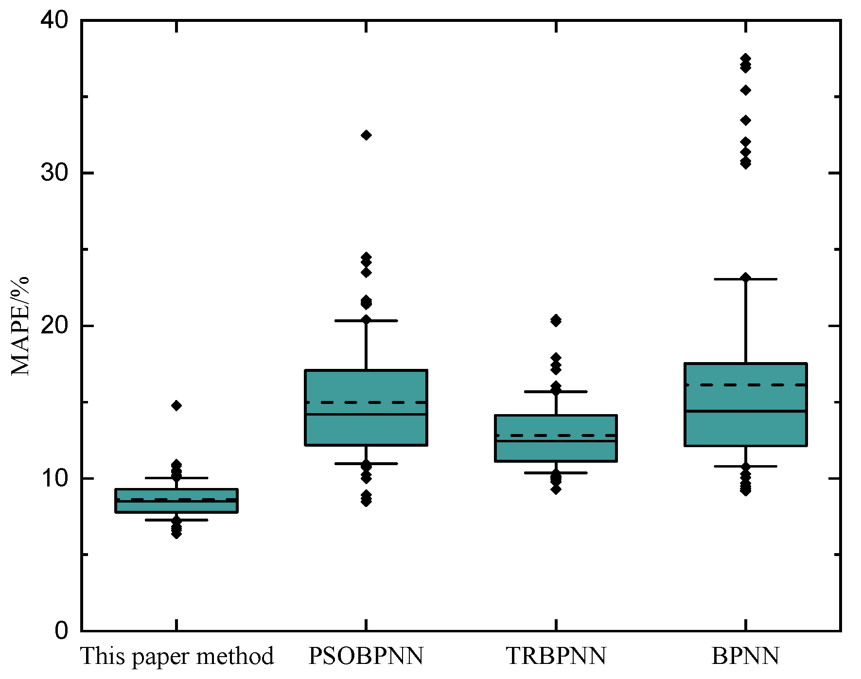
The method proposed in this paper demonstrated greater effectiveness compared to the other methods. The errors predicted by the comparison methods for the 40 sample points in the testing set are shown in Figure 7. In the figure, relative error values exceeding 20% are marked using circle points. It can be observed that the proposed method achieved superior prediction results except for sample points 1, 6, 9, 10, and 26. At sample points 1, 6, and 10, the errors were significant; nonetheless, the error values for the other models were also notable. This discrepancy may be attributed to the specific nature of the ship block constructions themselves. Two models outperformed the proposed method at sample points 9 and 26, indicating that there is still room for improvement in the proposed approach. Furthermore, a boxplot of the MAPE for the 100 experiments is shown in Figure 8. It is evident that the proposed method exhibited superior mean and median values and had more optimal, similar points, indicating better prediction accuracy and stability.

3.5. Comparison with Other Sample Capacities

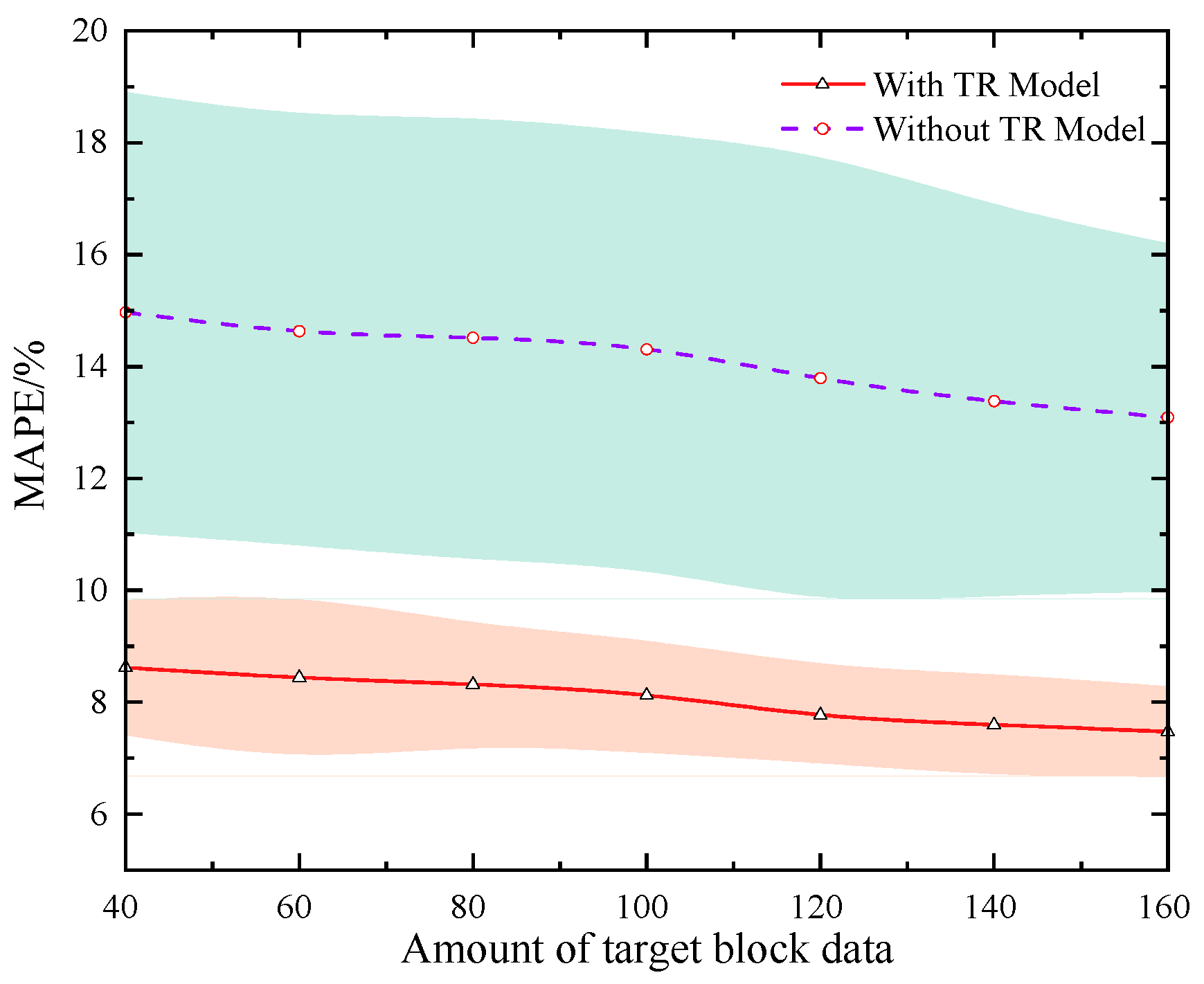
The prediction of target domain block time using 40 samples in this paper has already met the requirements for practical shipyard applications. To further demonstrate the superiority of the proposed method, different sample sizes were used to validate the model’s prediction. Out of the 200 target domain block samples, 160 were randomly selected to establish seven training sets containing 40, 60, 80, 100, 120, 140, and 160 samples, with the remaining 40 samples used as the test set. The effect of sample size on the MAPE of TR and non-TR models is shown in Figure 9. The lines represent the average MAPE values from 100 experimental runs, while the colored regions indicate the MAPE ranges. It is observed that the predictive performance of the model with-TR is significantly better than that without-TR. As the sample size increases, the average MAPE of both models decreases. Additionally, the fluctuation in the TR model is much smaller than in the without-TR model, indicating that the method proposed in this paper can effectively reduce the dispersion of the prediction results.

4. Discussion

Based on the experimental results, the proposed TR-PSO-BPNN model demonstrates a significant advantage in predicting ship block manufacturing times, surpassing other methods in both accuracy and stability. By leveraging clustering and transfer learning, the TR-PSO-BPNN model achieves improved prediction precision, especially when adapting to small sample sizes in the target domain. Clustering enhanced the prediction accuracy for source domain blocks, achieving an average MAPE of 9.5%, underscoring the value of the selected input features. Comparisons with non-clustering methods indicated that clustering is crucial for maintaining high accuracy across diverse manufacturing scenarios. Additionally, transfer learning—through selective weight freezing and fine-tuning—enabled the model to adapt more accurately to cruise ship blocks, with an average MAPE of 8.62%, markedly outperforming the non-transfer approach (14.97%) and highlighting the model’s adaptability.
Further comparisons with alternative models revealed that the TR-PSO-BPNN consistently delivered higher accuracy, with fewer extreme errors and reduced error dispersion, affirming its ability to capture the unique characteristics of ship block manufacturing. Testing with varying sample sizes also demonstrated the robustness of the transfer learning model; its performance improved steadily with sample size and showed less variability than models without transfer learning. This stability across sample sizes makes the TR-PSO-BPNN a reliable choice for shipbuilding production time forecasts.
Though developed for ship block time prediction, the TR-PSO-BPNN model also shows potential for broader applications, such as estimating maintenance durations by predicting equipment fatigue times, even for machinery with limited data, using insights from similar equipment. This adaptability could improve maintenance scheduling and resource allocation in ship operations. However, as the model’s effectiveness depends on the similarity between source and target domains, applications to new ship types or significantly different operational conditions may require additional data and model adjustments.

5. Conclusions and Future Work

The challenges posed by small sample datasets in ship block manufacturing have prompted the need for innovative time prediction methods. To address this, this paper presents a framework for ship block manufacturing time prediction, leveraging abundant historical data from source domain blocks to enhance predictions in target domain blocks. Extensive experimentation demonstrates the advantages of this framework under conditions of small sample datasets. The main points are summarized as follows:
The proposed block time prediction method in this paper achieves an MAPE value of 8.62%, whereas the block time prediction MAPE value for the BPNN model without the transfer learning algorithm is 14.97%. The introduction of transfer learning algorithms contributes significantly to improving the accuracy of ship block time prediction.
Comparative analysis reveals that the proposed method surpasses several others in terms of error values, means, and medians, indicating superior prediction accuracy and stability.
While the proposed method shows promise, further research is warranted. Firstly, a priority for future work will be to compare this transfer learning model against conventional models based on cross-domain datasets. This comparative study will enable a clearer assessment of the model’s adaptability and effectiveness across domains. Additionally, enhancing ease of use for practitioners is crucial; thus, developing user-friendly software that integrates the Python 3.11 scripts used in this research is also a practical future step. These planned developments aim to refine the model’s practical relevance and facilitate broader adoption.

Author Contributions

Conceptualization, J.L., P.L. and D.S.; methodology, J.L., P.L. and Z.Y.; software, P.L. and D.S.; validation, P.L. and D.S.; formal analysis, J.L., P.L. and D.S.; investigation, J.L. and Z.Y.; resources, J.L.; data curation, J.L. and Z.Y.; writing—original draft preparation, P.L. and B.Y.; writing—review and editing, P.L. and L.Z.; visualization, J.L., B.Y. and L.Z.; supervision, J.L.; project administration, J.L. and D.S. All authors have read and agreed to the published version of the manuscript.

Funding

This research was funded by the Ministerial Civil Ship Research Project of China (Grant number [2024]56).

Institutional Review Board Statement

Not applicable.

Informed Consent Statement

Not applicable.

Data Availability Statement

The data presented in this study are available on request from the corresponding author.

Acknowledgments

The authors thank Shanghai Waigaoqiao Shipbuilding Co., Ltd., for the support of operation data and verification scenarios.

Conflicts of Interest

Author Zhe Yan was employed by the company Shanghai Waigaoqiao Shipbuilding Co., Ltd. The remaining authors declare that the research was conducted in the absence of any commercial or financial relationships that could be construed as a potential conflict of interest.

References

  1. Back, M.G.; Lee, D.K.; Shin, J.G.; Woo, J.H. A study for production simulation model generation system based on data model at a shipyard. Int. J. Nav. Archit. Ocean Eng. 2016, 8, 496–510. [Google Scholar] [CrossRef]
  2. You-Ling, C.; Xiao-Jie, R.; Juan, T.; Hui-Cong, W. Labor hour estimation method based on difficulty coefficient of process in mass customization. Comput. Integr. Manuf. Syst. 2014, 20, 424–429. [Google Scholar]
  3. Kim, K.J.; Yun, W.G.; Kim, I.K. Estimating approximate construction duration of CFRD in the planning stage. KSCE J. Civ. Eng. 2016, 20, 2604–2613. [Google Scholar] [CrossRef]
  4. Choi, W.S.; Kim, D.H.; Nam, J.H.; Kim, M.J.; Son, Y.B. Estimating Production Metric for Ship Assembly Based on Geometric and Production Information of Ship Block Model. J. Mar. Sci. Eng. 2021, 9, 39. [Google Scholar] [CrossRef]
  5. Lei, Y.G.; Yang, B.; Jiang, X.W.; Jia, F.; Li, N.P.; Nandi, A.K. Applications of machine learning to machine fault diagnosis: A review and roadmap. Mech. Syst. Signal Proc. 2020, 138, 106587. [Google Scholar] [CrossRef]
  6. Wang, T.; Wang, J.B.; Zhang, X.J.; Liu, C. A Study on Prediction of Process Parameters of Shot Peen Forming Using Artificial Neural Network Optimized by Genetic Algorithm. Arab. J. Sci. Eng. 2021, 46, 7349–7361. [Google Scholar] [CrossRef]
  7. Yang, J.Y.; Kang, G.Z.; Liu, Y.J.; Kan, Q.H. A novel method of multiaxial fatigue life prediction based on deep learning. Int. J. Fatigue 2021, 151, 106356. [Google Scholar] [CrossRef]
  8. Rizaee, S.; Lei, Z. Duration Estimation of a Heavy Industrial Scaffolding Project: A Case Study. J. Constr. Eng. Manag. 2024, 150, 05024002. [Google Scholar] [CrossRef]
  9. Chang, J.T.; Kong, X.G.; Yin, L. A novel approach for product makespan prediction in production life cycle. Int. J. Adv. Manuf. Technol. 2015, 80, 1433–1448. [Google Scholar] [CrossRef]
  10. Kong, W.L.; Li, H. Combining adaptive time-series feature window and stacked bidirectional LSTM for predicting tool remaining useful life without failure data. Int. J. Adv. Manuf. Technol. 2022, 121, 7509–7526. [Google Scholar] [CrossRef]
  11. Chen, T.; Wang, Y.C. Estimating simulation workload in cloud manufacturing using a classifying artificial neural network ensemble approach. Robot. Comput. Integr. Manuf. 2016, 38, 42–51. [Google Scholar] [CrossRef]
  12. Chen, T. Incorporating fuzzy c-means and a back-propagation network ensemble to job completion time prediction in a semiconductor fabrication factory. Fuzzy Sets Syst. 2007, 158, 2153–2168. [Google Scholar] [CrossRef]
  13. Jeong, J.H.; Woo, J.H.; Park, J. Machine Learning Methodology for Management of Shipbuilding Master Data. Int. J. Nav. Archit. Ocean Eng. 2020, 12, 428–439. [Google Scholar] [CrossRef]
  14. Qu, S.P.; Jiang, Z.H. Man-hour calculation methods of the block assembly for shipbuilding. J. Harbin Eng. Univ. 2012, 33, 550–555. [Google Scholar]
  15. Zhu, H.; Woo, J.H. Hybrid NHPSO-JTVAC-SVM Model to Predict Production Lead Time. Appl. Sci. 2021, 11, 6369. [Google Scholar] [CrossRef]
  16. Li, J.H.; Sun, M.M.; Han, D.F.; Wang, J.X.; Mao, X.Z.; Wu, X.Y. A knowledge discovery and reuse method for time estimation in ship block manufacturing planning using DEA. Adv. Eng. Inform. 2019, 39, 25–40. [Google Scholar] [CrossRef]
  17. Liu, F.X.; Dai, Y.R. Product quality prediction method in small sample data environment. Adv. Eng. Inform. 2023, 56, 101975. [Google Scholar] [CrossRef]
  18. Kang, G.Q.; Wu, L.F.; Guan, Y.; Peng, Z. A Virtual Sample Generation Method Based on Differential Evolution Algorithm for Overall Trend of Small Sample Data: Used for Lithium-ion Battery Capacity Degradation Data. IEEE Access 2019, 7, 123255–123267. [Google Scholar] [CrossRef]
  19. Li, D.C.; Huang, W.T.; Chen, C.C.; Chang, C.J. Employing virtual samples to build early high-dimensional manufacturing models. Int. J. Prod. Res. 2013, 51, 3206–3224. [Google Scholar] [CrossRef]
  20. Li, D.C.; Lin, W.K.; Lin, L.S.; Chen, C.C.; Huang, W.T. The attribute-trend-similarity method to improve learning performance for small datasets. Int. J. Prod. Res. 2017, 55, 1898–1913. [Google Scholar] [CrossRef]
  21. El Bilali, A.; Taleb, A.; Bahlaoui, M.A.; Brouziyne, Y. An integrated approach based on Gaussian noises-based data augmentation method and AdaBoost model to predict faecal coliforms in rivers with small dataset. J. Hydrol. 2021, 599, 126510. [Google Scholar] [CrossRef]
  22. Zhuang, F.Z.; Qi, Z.Y.; Duan, K.Y.; Xi, D.B.; Zhu, Y.C.; Zhu, H.S.; Xiong, H.; He, Q. A Comprehensive Survey on Transfer Learning. Proc. IEEE 2021, 109, 43–76. [Google Scholar] [CrossRef]
  23. Moreo, A.; Esuli, A.; Sebastiani, F. Lost in Transduction: Transductive Transfer Learning in Text Classification. ACM Trans. Knowl. Discov. Data 2022, 16, 1–21. [Google Scholar] [CrossRef]
  24. Zhuang, F.Z.; Luo, P.; Du, C.Y.; He, Q.; Shi, Z.Z.; Xiong, H. Triplex Transfer Learning: Exploiting Both Shared and Distinct Concepts for Text Classification. IEEE Trans. Cybern. 2014, 44, 1191–1203. [Google Scholar] [CrossRef]
  25. He, X.; Chen, Y.S.; Ghamisi, P. Heterogeneous Transfer Learning for Hyperspectral Image Classification Based on Convolutional Neural Network. IEEE Trans. Geosci. Remote Sens. 2020, 58, 3246–3263. [Google Scholar] [CrossRef]
  26. Wang, D.; Zheng, T.F. Transfer Learning for Speech and Language Processing. In Proceedings of the Asia-Pacific-Signal-and-Information-Processing-Association Annual Summit and Conference (APSIPA ASC), Hong Kong, China, 16–19 December 2015; pp. 1225–1237. [Google Scholar]
  27. Zhou, H.T.; Chen, J.; Dong, G.M.; Wang, R. Detection and diagnosis of bearing faults using shift-invariant dictionary learning and hidden Markov model. Mech. Syst. Signal Proc. 2016, 72–73, 65–79. [Google Scholar] [CrossRef]
  28. Mao, W.T.; Ding, L.; Tian, S.Y.; Liang, X.H. Online detection for bearing incipient fault based on deep transfer learning. Measurement 2020, 152, 107278. [Google Scholar] [CrossRef]
  29. Li, Q.; Shen, C.Q.; Chen, L.; Zhu, Z.K. Knowledge mapping-based adversarial domain adaptation: A novel fault diagnosis method with high generalizability under variable working conditions. Mech. Syst. Signal Proc. 2021, 147, 107095. [Google Scholar] [CrossRef]
  30. Yang, B.; Xu, S.C.; Lei, Y.G.; Lee, C.G.; Stewart, E.; Roberts, C. Multi-source transfer learning network to complement knowledge for intelligent diagnosis of machines with unseen faults. Mech. Syst. Signal Proc. 2022, 162, 108095. [Google Scholar] [CrossRef]
  31. Zhang, A.S.; Wang, H.L.; Li, S.B.; Cui, Y.X.; Liu, Z.H.; Yang, G.C.; Hu, J.J. Transfer Learning with Deep Recurrent Neural Networks for Remaining Useful Life Estimation. Appl. Sci. 2018, 8, 2416. [Google Scholar] [CrossRef]
  32. Sun, C.; Ma, M.; Zhao, Z.B.; Tian, S.H.; Yan, R.Q.; Chen, X.F. Deep Transfer Learning Based on Sparse Autoencoder for Remaining Useful Life Prediction of Tool in Manufacturing. IEEE Trans. Ind. Inform. 2019, 15, 2416–2425. [Google Scholar] [CrossRef]
  33. Hung, S.K.; Gan, J.Q. Small facial image dataset augmentation using conditional GANs based on incomplete edge feature input. PeerJ Comput. Sci. 2021, 7, e760. [Google Scholar] [CrossRef]
  34. Zhao, W. Research on the Deep Learning of the Small Sample Data based on Transfer Learning. In Proceedings of the International Conference on Green Energy and Sustainable Development (GESD), Chongqing, China, 27–28 May 2017. [Google Scholar]
  35. Chen, J.G.; Han, X.B.; Sun, T.; Zheng, Y.J. Analysis and prediction of battery aging modes based on transfer learning. Appl. Energy 2024, 356, 122330. [Google Scholar] [CrossRef]
  36. Li, J.H.; Guo, D.; Chen, Z.Y.; Li, X.; Li, Z.F. Transfer learning for collapse warning in TBM tunneling using databases in China. Comput. Geotech. 2024, 166, 105968. [Google Scholar] [CrossRef]
  37. Li, Y.; Wei, P.T.; Xiang, G.; Jia, C.F.; Liu, H.J. Gear contact fatigue life prediction based on transfer learning. Int. J. Fatigue 2023, 173, 107686. [Google Scholar] [CrossRef]
  38. Kretschmer, R.; Pfouga, A.; Rulhoff, S.; Stjepandic, J. Knowledge-based design for assembly in agile manufacturing by using Data Mining methods. Adv. Eng. Inform. 2017, 33, 285–299. [Google Scholar] [CrossRef]
  39. Deng, Z.H.; Jiang, Y.Z.; Chung, F.L.; Ishibuchi, H.; Choi, K.S.; Wang, S.T. Transfer Prototype-Based Fuzzy Clustering. IEEE Trans. Fuzzy Syst. 2016, 24, 1210–1232. [Google Scholar] [CrossRef]
  40. Sun, Y.; He, D.P.; Li, J. Research on the Fatigue Life Prediction for a New Modified Asphalt Mixture of a Support Vector Machine Based on Particle Swarm Optimization. Appl. Sci. 2021, 11, 11867. [Google Scholar] [CrossRef]
  41. Xiao, M.Z.; Luo, R.; Chen, Y.; Ge, X.M. Prediction model of asphalt pavement functional and structural performance using PSO-BPNN algorithm. Constr. Build. Mater. 2023, 407, 133534. [Google Scholar] [CrossRef]
  42. Geyer, P.; Schlüter, A.; Cisar, S. Application of clustering for the development of retrofit strategies for large building stocks. Adv. Eng. Inform. 2017, 31, 32–47. [Google Scholar] [CrossRef]
  43. Golizadeh, H.; Sadeghifam, A.N.; Aadal, H.; Abd Majid, M.Z. Automated tool for predicting duration of construction activities in tropical countries. KSCE J. Civ. Eng. 2016, 20, 12–22. [Google Scholar] [CrossRef]
  44. Min, C.; Bin, P.; Jian, L. Man-hour Calculation of Working Package using Error Back-propagation Artificial Neural Network. Shipbuild. China 2003, 44, 1–7. [Google Scholar]
  45. Ruy, W.S.; Kim, H.K.; Cho, Y.J.; Ko, D.E. Implementation of welding material quantity evaluation system combined with ship design CAD system. Int. J. Nav. Archit. Ocean Eng. 2017, 9, 219–226. [Google Scholar] [CrossRef]
  46. Bezdek, J.C. Pattern Recognition with Fuzzy Objective Function Algorithms; Siam Review: Philadelphia, PA, USA, 1983; Volume 25. [Google Scholar]
  47. Hornik, K.; Stinchcombe, M.; White, H. Multilayer feedforward networks are universal approximators. Neural Netw. 1989, 2, 359–366. [Google Scholar] [CrossRef]
  48. Karch, J. Improving on Adjusted R-Squared. Collabra-Psychol. 2020, 6, 45. [Google Scholar] [CrossRef]
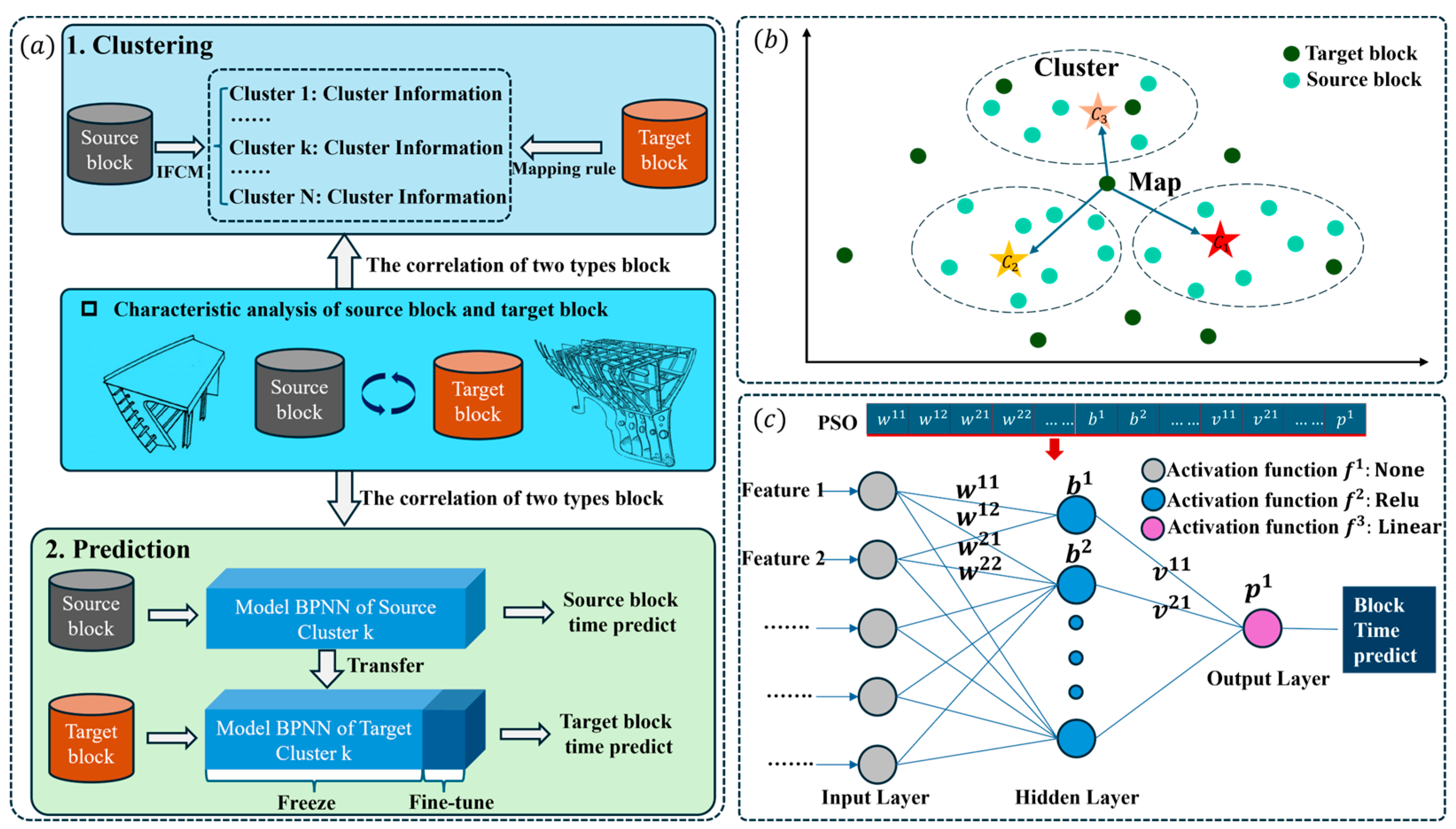
Figure 1. (a) The framework of block time prediction; (b) cluster process; (c) PSO-BPNN framework.
Jmse 12 01977 g001
Figure 2. Prediction flow chart of TL-PSO-BPNN model.
Jmse 12 01977 g002
Figure 3. Source block time prediction results of (a) MAPE values and (b) R a d j 2 values.
Jmse 12 01977 g003
Figure 4. Parameter freezing and fine-tuning information of TR-PSO-BPNN.
Jmse 12 01977 g004
Figure 5. Comparisons of target block time predict results: (a) with-TR models; (b) without-TR models.
Jmse 12 01977 g005
Figure 6. Comparison of different methods and true values.
Jmse 12 01977 g006
Figure 7. Comparison of different methods: absolute errors.
Jmse 12 01977 g007
Figure 8. Comparison of different methods: MAPE.
Jmse 12 01977 g008
Figure 9. The effect of sample size on the MAPE of TR and without-TR models.
Jmse 12 01977 g009
Table 1. Block features for clustering.
No.Feature NameData TypeRange
1Block weightNumeric[120, 240]
2Block projection areaNumeric[110, 280]
3Unit assembly block numberNumeric[7, 28]
4Block typeEnumerationsuch as curved block, flat block, two-dimensional unit, and volume surface section
5Slope typeEnumerationsuch as I, X, Y, V, K, and U slopes
6Welding seam typeEnumerationsuch as butt weld, filet weld, and lap weld
Table 2. Neural network hyperparameters of the PSO-BPNN model selection.
HyperparametersSize of Value
The number of input layer nodes5
The number of hidden layers1
The number of hidden layer nodes4
The number of output layer nodes1
The total trainable parameters29
Initialization minimum error1 × 105
The   activation   function   f 2 R e l u
The   activation   function   f 3 L i n e a r
The loss functionMean Square Error
The number of trainings200
Minimum error of training target1 × 10−6
Table 3. PSO algorithm hyperparameters of the PSO-BPNN model selection.
HyperparametersSize of Value
Individual and group learning factors1.5
Maximum number of iterations200
Particle swarm size200
Minimum value of inertia weight0.4
Maximum value of inertia weight0.9
Speed limit range[−3, 3]
Location restrictions[−5, 5]
Individual and group learning factors1.5
Table 4. Block clustering results.
Cluster1Cluster2Cluster3Cluster4
Source block count191192463154
Target block count31479626
Disclaimer/Publisher’s Note: The statements, opinions and data contained in all publications are solely those of the individual author(s) and contributor(s) and not of MDPI and/or the editor(s). MDPI and/or the editor(s) disclaim responsibility for any injury to people or property resulting from any ideas, methods, instructions or products referred to in the content.