Abstract
Ship piping arrangement is a nondeterministic polynomial problem. Based on the advantages of the grey wolf optimization (GWO) algorithm, which is simple, easy to implement, and has few adjustment parameters and fast convergence speed, the study adopts the grey wolf optimization (GWO) algorithm to solve the ship piping arrangement problem. First, a spatial model of ship piping arrangement is established. The grid cell model and the simplified piping arrangement environment model are established using the raster method. Considering the piping arrangement constraint rules, the mathematical optimization model of piping arrangement is constructed. Secondly, the grey wolf optimization algorithm was optimized and designed. A nonlinear convergence factor adjustment strategy is adopted for its convergence factor. Powell’s algorithm is introduced to improve its local search capability, which solves the problem that the grey wolf algorithm easily falls into the local optimum during the solving process. Simulation experiments show that compared with the standard grey wolf algorithm, the improved algorithm can improve the path layout effect by 38.03% and the convergence speed by 36.78%. The improved algorithm has better global search ability, higher solution stability, and faster convergence speed than the standard grey wolf optimization algorithm. At the same time, the algorithm is applied to the actual ship design, and the results meet the design expectations. The improved algorithm can be used for other path-planning problems.
1. Introduction
Oil, water, and electricity are transported to various compartments onboard a ship through the piping system. Therefore, the piping system is the ship’s blood vessels. The layout of the piping system directly affects the working efficiency, safety, and aesthetics of the ship. The traditional piping design process requires designers to constantly modify and adjust, which consumes a lot of time and labor costs. According to the survey, the workload of ship piping layout accounts for about half of the total workload of the piping detailed design stage. It takes 30,000 to 40,000 working hours to design the pipeline layout of a ship of medium complexity [1]. Optimizing the comprehensive design of ship pipelines is not only about minimizing the length of the pipelines but also about optimizing the economic, aesthetic, practical, and other aspects so that the ship can better perform its functions and provide better services. Therefore, the ship 3D pipeline optimization layout problem is similar to path optimization, and an intelligent pipeline layout method needs to be investigated.
Unlike intelligent design technology, traditional ship piping design is based on design manuals and specifications, along with experience accumulation and reference drawings. The traditional design method is inefficient and ineffective. Intelligent layout design is able to realize automated layout scheme output with the addition of computers and algorithms. Automatic piping layout design is the process of solving for feasible piping layout results within given geometric, topological, technical, and rule constraints. Geometrically, it is to find a path that does not interfere with other objects, satisfies various constraints, and goes to a specified endpoint from a specified starting point in a restricted layout space. The problem is similar to the robot path-finding problem in 3D space and belongs to the NP-hard combinatorial optimization problems.
Due to the highly complex spatial layout of piping inside a ship and the many related layout requirements, human design has the disadvantages of inefficiency, high dependence on experience, and poor quality of the piping layout. To solve the above problems, in recent years, relevant researchers at home and abroad have carried out in-depth research on the intelligent arrangement of ship pipelines based on optimization algorithms, and the methods used can be broadly divided into deterministic algorithms, non-deterministic algorithms, i.e., heuristic algorithms, and hybrid algorithms fused by the two, and so on. In determining the algorithm, Lee proposed the maze algorithm, which guarantees the shortest path while avoiding obstacles [2]. However, the computation time of the maze algorithm is slow, and when the constraints reach a certain number, the algorithm’s complexity will greatly increase. To overcome its drawbacks, Hightower proposed an escape algorithm (escape algorithm) [3]. However, its results cannot always find the optimal value, so the algorithm’s operation is generally associated with the Memetic Algorithm (MA). Lu et al. proposed a hybrid escape and maze algorithm with partitioned and hierarchical sequential placement [4]. However, the algorithm is less generalized and only considers the cost of line lengths, not other factors such as corners, equipment types, etc. Bian et al. improved the traditional A-star algorithm for the ship piping arrangement problem [5]. However, this method cannot provide multiple schemes for optimization, and the probability of searching for the optimal piping arrangement scheme is low. Burdorf et al. and Kaniat proposed deterministic algorithms for different arrangement conditions [6,7]. Overall, while the deterministic algorithm is more efficient in pipeline placement, it has fixed results that cannot be subsequently optimized, and the algorithm has low adaptability.
Addressing the limitations of the deterministic approach, the intelligent algorithms provide good ideas and directions for pipe path routing. A large number of intelligent algorithms are used to solve pipeline design problems, such as the Genetic Algorithm (GA) [8,9,10,11], Particle Swarm Optimization (PSO) algorithm [12], Ant Colony Algorithm(ACA) [13], heuristic algorithm [14], and differential evolution and cuckoo search [15]. The above algorithms have problems when applied to piping arrangements. For example, based on the improved particle swarm algorithm, Dong et al. proposed an algorithmic framework for the cooperative arrangement of multiple pipelines or branch pipelines [12]. The simulation results show that the quality of pipeline arrangement is poor, and there is still much room for improvement. In the optimization design of multi-pipes for ships, Jiang et al. proposed a co-evolutionary improved multi-ant colony optimization (CIMACO), which achieves better performance in avoiding local optimums and accelerating the convergence speed [16]. However, there is a problem of decreasing the efficiency and quality of pipeline arrangements when the population size increases. In terms of hybrid algorithms, Sui and Dong et al. combined the maze algorithm and A* algorithm on the framework of the genetic algorithm to solve the automatic pipeline arrangement problem [17,18]. However, the algorithm’s complexity is high, and its solution is less efficient.
Generally speaking, the above algorithms can help piping designers automatically arrange pipelines, so they are called intelligent pipeline arrangement algorithms. In comparison, the deterministic algorithms are more efficient for piping layout, but the results are not necessarily preferable; the heuristic algorithms provide multiple solutions for piping layout, but they take longer to run and solve. Because the piping arrangement problem belongs to the NP-hard problem, the spatial and temporal complexity is huge when solving the large-scale problem. In practical engineering applications, it is often not required to find the optimal solution of the problem, and it is expected that a feasible near-optimal solution (satisfactory solution) can be obtained in a short time. Non-deterministic algorithms have an irreplaceable role in solving the pipeline layout problem and can be directly used to search for the pipeline path, but they can also be used to optimize the pipeline laying order. With the in-depth study of piping arrangement, researchers have realized that there is no universal method that can be applied to all kinds of piping arrangement requirements for such a complex problem as the piping arrangement of ships, and it is often necessary to choose different optimization methods according to the situation [1]. In other words, a single solution method has limitations, and designers must select appropriate algorithms for solving different requirements. Currently, there is no mature commercial CAD software to support the automated layout of ship piping, mainly because the ship piping layout is characterized by customization (the piping layout needs vary greatly among ship products). Although it is a great challenge to develop software to meet the actual ship design applications, it is important to study the automated arrangement of ship piping to promote the development of digital shipbuilding.
Considering the deterministic algorithms, although the solution efficiency is higher, only a single fixed solution can be obtained, and the form of constraints considered is more straightforward. The initialization process of meta-heuristic and hybrid algorithms needs to rely on manual experience to set multiple optimization parameters, and their solution quality is greatly affected by the parameter values; there is a large order of magnitude difference in the weight system corresponding to different optimization objectives, which needs to be re-adjusted when solving different ship piping arrangement problems, and the robustness is low. They cannot obtain the corresponding arrangement scheme according to the designers’ different practical needs. Therefore, the grey wolf algorithm is introduced to solve piping arrangement problems, and the application value of the grey wolf algorithm is explored in piping arrangement problems.
GWO (grey wolf optimization) achieves optimization by simulating the predation behavior of grey wolf populations and utilizing the mechanism of wolf group collaboration [19]. This mechanism has achieved good results in balancing exploration and development and has good performance in convergence speed and solution accuracy. It has been widely used in the engineering field. The GWO search process, like other swarm intelligence (SI)-based algorithms [20], begins with the random creation of a population. It starts with the random creation of populations. Then, four groups of wolves and their locations are formed, and their distance to the target prey is measured. Each individual represents a candidate solution and is updated through iterative search. In addition, GWO employs two control parameters to maintain strong exploration and exploitation capabilities, effectively avoiding local optimum stagnation. Although GWO’s approach to approximating the global optimum is similar to other population-based algorithms, the mathematical model of the algorithm is novel. There is only one position vector in the GWO algorithm, so it requires less computer memory than the PSO algorithm, which has both position and velocity vectors. The advantages of GWO make it one of the fastest-growing population-based intelligent optimization algorithms today.
Currently, this algorithm is mostly used for robot path planning at a two-dimensional level, similar to the pipeline layout problem [21,22,23,24,25]. For the traditional GWO algorithm, there are the problems of easily being trapped in the local optimum, and the algorithm’s ability to find the optimum is weakened in the later stage, and there is a huge room for improvement, especially for the pipeline layout optimization problem, which can be improved in the pathfinding and the logic of the algorithm so as to enhance the quality of the solution and the algorithm’s convergence speed, and the algorithm has a great potential for improvement.
In this paper, for the pipeline path planning problem in the ship pipeline system, with the main goal of obtaining the optimal pipeline path layout scheme by optimization calculation, the ABC algorithm is used to solve the optimization problem, and the defects of the basic GWO algorithm are improved. At the same time, an optimization algorithm adapted to solve the optimization of pipeline paths is proposed by combining it with the Powell algorithm [26]. Finally, the feasibility and efficiency of the algorithm are verified by engineering cases. The paper is structured as follows: Section 1 is an introduction and Section 2 presents the mathematical model of pipeline optimization. Section 3 presents the GWO algorithm and its improvements. Section 4 provides a case study to validate the proposed method. Finally, the paper ends in Section 5 and gives conclusions.
2. Description of Ship Pipeline Layout Problem
Ship piping is usually connected to equipment or valves. In order to ensure that the automatic layout is out of a collision-free reasonable pipeline, the automatic layout of piping is divided into two steps.
- (1)
- According to the ship’s equipment layout characteristics, consider the valve, equipment location, and other factors in the establishment of a pipeline layout environment map.
- (2)
- Search algorithms are used to search for pipelines in the environment map.
The overall solution for the ship pipeline layout method is shown in Figure 1.
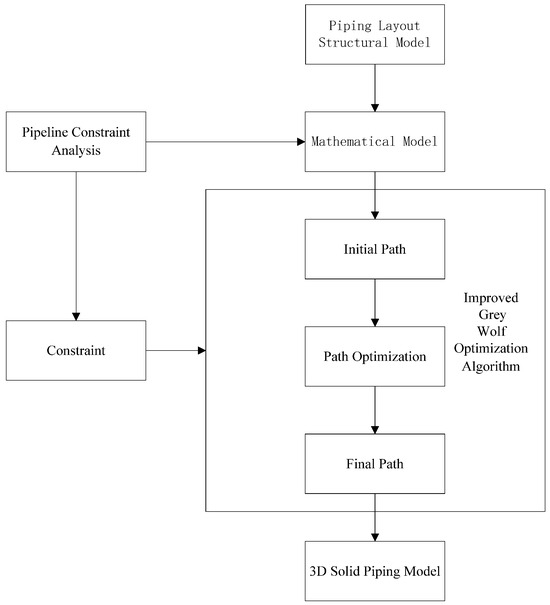
Figure 1.
The overall solution for ship pipeline layout.
In the solution of Figure 1, the first step is to obtain a 3D pipeline layout structure model, whose main purpose is to simplify the ship pipeline layout environment. In other words, a ship pipeline layout space is created. The solution space of the mathematical model is finally obtained. Then, the constraint information of the pipeline is analyzed and the engineering constraints are mathematically modeled to construct the constraints in the pipeline path planning process. From the perspective of piping engineers or layout algorithms for laying piping, three types of constraints should be considered to be satisfied during the ship piping layout process: general constraints, system relevance constraints, and environment relevance constraints. General constraints are a class of constraints by which each pipeline or the vast majority of pipeline layouts are affected. For example: Minimum safety distance should be guaranteed between piping and piping, piping and equipment. System relevance constraints are a class of arrangement constraints imposed by the ship’s functional system to which the piping to be arranged belongs on the associated piping, and the rules of this class are related to the system to which the piping belongs. For example, for heavy and large system piping, the center of gravity of the arrangement should be as low as possible to help the ship maintain balance. Environmental relevance constraints are a class of layout constraints imposed by the current layout space environment on the pipelines located therein. For example, there must be no safety hazards between neighboring pipelines or between a pipeline and the equipment or environment through which it passes. The general constraints are relatively stable and can be solidified into the layout space model or algorithmic logic to be realized. The system relevance constraints and environment relevance constraints are dependent on the piping system to be laid out and the layout environment, which needs to be supported by the automated piping layout algorithms to dynamically update these two types of constraints, which can be added before laying out the corresponding piping and then removed after the layout is completed. On this basis, the ship design process is transformed into a reasonable mathematical model, and intelligent design is carried out based on this mathematical model. The process focuses on determining the objective function. After that, the algorithm proposed in this paper is used to optimize the pipeline arrangement in the feasible space, and the optimal pipeline path is obtained. Finally, the virtual 3D solid pipeline model can be generated based on the optimal path. In addition, since the optimization process is carried out in the feasible grid, the algorithm can ensure that the paths are always in the possible space during the path search and optimization process.
2.1. Ship Pipeline Layout Space
Ship piping is arranged in compartments. The arrangement of cabins usually requires consideration of the function of the cabin. Therefore, the cabins usually contain many equipment and personnel passages. To facilitate the conversion of the actual physical environment of a cabin into a digital environment that a computer can process, this paper adopts the raster method proposed by Howden W E [27]. This method represents the environment map by raster, which reduces the computation and complexity of the obstacle boundary information processing in the pipeline path planning process and improves the efficiency of pipeline path search. The entire layout space can be regarded as a rectangular prism. Using the grid method for grid division, the layout space can be divided into several equally sized cubes, also known as grid cells, as shown in Figure 2, and each grid node is labeled with coordinates. Normally, we do not arrange space as a regular cube. In this case, we can expand it into a cube with minimal padding, treating the expanded part as an obstacle and assigning it a value of 1, while assigning a value of 0 to non-obstacles. In the process of grid partitioning, when the grid partitioning is sufficiently small, the layout environment will infinitely approach the real layout environment, and the accuracy of the established model will be high, which will increase the amount of data and prolong the iterative optimization time. When the partition is too large, the environmental resolution will be very low, and the model accuracy will be low. Here are several factors to consider when setting the grid size d.
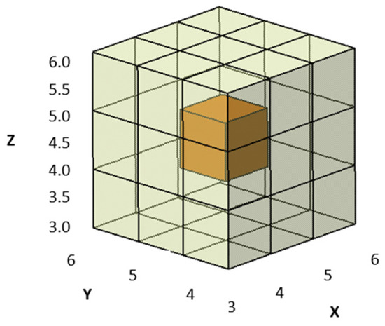
Figure 2.
Grid method for dividing space 1.
- ➀
- Pipeline radius ε: In the pipeline layout, the centerline will be used to represent the layout. If the grid size is smaller than the pipeline radius, it may cause errors. So the grid size is d ≫ ε.
- ➁
- Reserved gap between pipelines: When arranging pipelines, the gap between adjacent pipelines should not be less than 20mm for pipeline installation, maintenance, and insulation. So the grid size is d ≫ ε + γ.
- ➂
- Reserved gap between pipeline and obstacle: In actual layout, a gap will be reserved between pipeline and obstacle, and adjusted according to actual use. When arranging a single pipeline, the grid size should be d ≫ ε + δ. In a multi-pipeline layout, the larger one can be selected and adjusted according to the actual situation.
In this paper, the grid is mainly based on the internal equipment of the compartment, and bulkhead edge to divide. Compartment equipment, bulkheads, decks, personnel access, etc. is equivalent to the grid, in which the equipment, personnel access, etc. for the impenetrable grid, bulkheads, and decks can be based on the actual situation to determine whether it is possible to penetrate. The algorithm performs a pipeline search in the penetrable grid.
The pipeline model refers to the use of mathematical or physical methods to model pipelines in computer programs for computer simulation and analysis. In engineering design, pipeline models are commonly used to analyze issues such as pipeline fluid dynamics, heat transfer, and mass transfer. According to specific problem requirements, pipeline models can be modeled using different mathematical methods, such as ordinary differential equations, partial differential equations, etc. In computer programs, pipeline models are typically viewed as a network consisting of several nodes and segments. Each node represents a location where changes in physical quantities such as flow, temperature, and pressure can occur. Each pipe segment represents a section of the pipeline between two nodes, and the fluid in the pipeline can be affected by various external factors such as gravity, inertia, friction, etc. By establishing such a pipeline model, various calculations and analyses can be carried out, such as flow rate, pressure, temperature distribution, etc. This article simplifies the pipeline using its centerline.
2.2. Description of the Pipe Layout Problem
The pipe layout problem can be viewed as a rigid robot planning its motion in the layout space and finding a touchless path from the start point to the endpoint, whose mathematical description is shown in Figure 3.
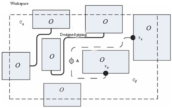
Figure 3.
Description of the piping layout problem.
The workspace of the pipeline path problem is denoted by W, , which contains not only all the mechanical parts of the initial product, assembly fixtures and clamps, workbench, etc., but also the pipeline and its attachments and other items, for which the layout has been completed. Among them, the rigid robot for motion planning is denoted by A, and the obstacles in the planning space are denoted by O, .
Generally speaking, the cross-section of the pipeline is a constant circle. Therefore, the rigid robot for path planning can be set as a spherical rigid body. The trajectory of its spherical center is the centerline of the pipeline. The swept trajectory of the rigid body is the initial path of the pipeline. In the pipeline path-solving calculation process, the flow shape generated by the spherical rigid body transformation is a three-dimensional flow shape. Therefore, the state space for solving the path planning problem is three-dimensional, denoted by , . is the set of all feasible solutions in the state space. This space is called the free space. Any solution in is denoted by x, .
Before the pipe path-solving computation, a start point and an end point () are input. Then, a series of discrete path nodes are obtained after initialization computation, which contain the position information of the spherical rigid body. Finally, these discrete points are optimized to obtain the final pipe path.
2.3. Mathematical Model
2.3.1. Encoding Method
For the problem of pipeline path planning, the expression of one solution corresponding to one path will be adopted in this paper in the form of fixed-length coding, with the three-dimensional coordinates of the nodes through which the path passes as the basic unit. So, the encoding method of a path can be represented as
where , are the three-dimensional coordinates of the starting and ending points of the pipeline, and the remaining points represent the nodes that the pipeline path passes.
2.3.2. Objective Function
The objective function of the path optimization problem studied in this article mainly considers the following five aspects.
- (1)
- Path length function.
- (2)
- Number of elbows function.
The number of elbows function is represented by B(x), which represents the number of elbows in a path. When determining whether a middle node of a path is an elbow, it is necessary to coordinate the positions of the two nodes before and after the node to make the judgment. If the three points are on the same straight line, the middle node is a non-elbow point; otherwise, it is an elbow. Assuming that the node to determine whether it is an elbow is p, and its front and rear nodes are p1 and p2, respectively, use Equations (3) and (4) to calculate the unit vector e1 between p1 and p and the unit vector e2 between p and p2, respectively.
where is the three-dimensional coordinate of point p; are the three-dimensional coordinates of point p1 and point p2, respectively.
Calculate the number of bends function using Equation (5).
where np is the number of nodes in the path.
- (3)
- Orthogonal function.
- (4)
- Energy zone function.
The energy region function is represented by E(x). In the three-dimensional space of pipeline layout, it is generally preferred to lay pipelines around obstacles, map boundary areas, and set these areas as energy zones. The energy zone around the obstacle is set, as shown in the figure. The energy zone function represents the length of the pipeline path passing through the energy zone, and the calculation formula is shown in Equation (7). The larger the calculation result, the more energy zones the pipeline passes through, and the better the layout effect.
where is the path length of the energy zone passed through in the i-th segment of the path.
- (5)
- Penalty function.
The penalty function, represented by P(x), is used to punish unreasonable situations in the path, such as interference with obstacles and path reversal.
- (6)
- Overall objective function
Based on the objective function expressed in the above equation, the overall objective function of the pipeline optimization problem, which is the fitness function, can be obtained as shown in Equation (8).
where are weight coefficients aimed at controlling the weight ratio of the five sub-objective functions in the algorithm.
From the optimization problem expression (1) and the overall objective function Equation (8), it can be seen that this paper transforms the multi-objective optimization of pipeline path optimization into a single objective optimization problem, which is a minimum value optimization problem. That is, the smaller the value of F(x), the better the layout effect of the pipeline. Due to the different units and significant numerical differences in the calculation results of each sub-objective function, to more reasonably express the role of each sub-objective function in the optimization process, Equation (9) is used to make dimensionless some sub-objective functions so that their values are within the range of [0, 1].
where and are the minimum and maximum values taken by the objective function calculation results, respectively.
The summary of the data factorization methods for each sub-objective function is as follows.
For the path length function, is expressed as the straight line distance between the starting points of the pipeline; is expressed as the maximum of all path lengths in the initial population.
For the number of bends function, is taken to be 0, indicating that the path has no elbows; is expressed using the maximum value of the number of elbows of all paths in the initial population.
For the orthogonality function, is taken to be 0, indicating that the paths are all arranged orthogonally; is expressed as the maximum orthogonality value of all paths in the initial population.
In particular, for the energy function and the penalty function, they are treated according to Equations (10) and (11), respectively.
The equation represents the ratio of the path length passing through the energy zone in the current path to the total path length, where L denotes the total path length.
If there is an irrational situation in the path, the penalty function after factorization takes 1, and the opposite takes 0.
2.3.3. Constraint Condition
In the actual ship pipeline layout, numerous constraints and objectives cannot be fully considered by algorithms. Therefore, this article only deals with objectives and constraints that are easy to quantify and solve by algorithms. In practical work, pipeline designers also need to combine manual experience to select the results further. Constraints:
- (1)
- Connectivity should be ensured between the pipeline’s starting points. Connectivity belongs to the physical constraints of the pipeline layout. The pipeline’s path should ensure that the front and back between the starting point of the path cannot be interrupted.
- (2)
- Pipelines and obstacles (cabin structure, equipment, laid-out pipelines, reserved space, etc.) do not collide. Assuming that the pipeline passes through a total of n path nodes and there are m obstacles in the layout space, to satisfy the physical constraints that the pipeline does not interfere with the obstacles, the situation shown in Equation (11) should be avoided.
- (3)
- Piping layout should ensure orthogonality. To meet the production constraints, the pipeline should be arranged orthogonally in the layout space to avoid a situation where it goes diagonally.
- (4)
- Piping should be as much as possible in the energy zone. To meet the production and safety constraints, most of the pipelines are expected to be arranged close to the equipment or bulkheads. In contrast, a few pipelines must be located far away from certain equipment. For example, locating pipelines transporting fuel oil above the boiler should be avoided. These constraints can be met through the installation of energy zones.
Optimization objective:
- (1)
- Path lengths are kept as short as possible in order to satisfy economic constraints and to reduce pipelaying costs.
- (2)
- The number of elbows is kept as low as possible in order to satisfy economic constraints and to reduce the cost of laying pipes.
- (3)
- The pipeline should be arranged as close as possible to the supporting surface (bulkhead, floor, specific equipment) for easy installation.
- (4)
- The pipeline path should avoid the “concave pocket” structure (U-shaped path in the vertical direction) as much as possible to reduce medium blockage.
- (5)
- The distance between adjacent bends of pipelines shall not be less than the specified length to meet processing constraints or reduce processing costs.
3. Intelligent Solving Algorithms
3.1. Grey Wolf Optimization Algorithm
The grey wolf optimization algorithm simulates the hunting behavior and hierarchy of grey wolves in nature [19]. In the grey wolf optimization algorithm, α leads the hunting action, β assists in decision-making, δ arranges specific actions, and ω follows the instructions of the first three to track and encircle the prey, ultimately completing the hunting action.
When using the grey wolf optimization algorithm to solve optimization problems in the G-dimensional search space, it is assumed that the number of grey wolf individuals in the grey wolf population is N, where the position of the i-th grey wolf in the G-dimensional space can be represented as , the current optimal individual in the population is denoted as α, the current suboptimal individual is denoted as β, the current third most optimal individual is denoted as δ, and the remaining individuals are denoted as ω. The prey’s position corresponds to the optimization problem’s global optimal solution. The optimization process of the grey wolf optimization algorithm is to randomly generate a group of grey wolf individuals in the search space, evaluate the fitness of this group of grey wolf individuals, and obtain the top three grey wolf individuals in fitness, α, β, and δ, which are used as the positions for finding prey. The benchmark for the global optimal solution is to calculate the position of the next generation of grey wolf individuals based on the positions of α, β, and δ.
During the hunting process, the grey wolf population must first take a surrounding action towards the prey. Correspondingly, in the optimization process of the grey wolf optimization algorithm, the distance between the individual and the prey must be determined. In grey wolf hunting, the act of encircling prey is defined as
Equation (12) is the distance equation between individual wolves and the target, and Equation (13) is the position update equation for gray wolves, where and are the position vectors of the target and the grey wolf, respectively; t is the number of iterations; and are the coefficient vectors; and the equation is
where is the convergence factor, which decreases linearly from 2 to 0 with the number of iterations; random numbers between [0, 1]. is the maximum number of iterations.
In the grey wolf population, α wolves, β wolves, and δ wolves are the groups that are closest to the prey and most able to perceive the prey information, and the positions of the rest of the individual gray wolves are determined based on these three species.
In the actual path planning, α, β, δ are the three optimal solutions obtained so far, and the positions of these three are used to determine the position of the next target and force the rest of the gray wolves to update their positions according to the positions of the optimal gray wolves, and the mathematical model is
Equation (18) defines the distance between α, β, δ, and other individuals, represent the current position of α, β, δ, respectively, and is the current target position vector. Equation (19) defines the step size and distance of ω moving toward α, β, δ, and Equation (20) is the final position of ω.
3.2. Pseudo-Code for the Grey Wolf Optimization Algorithm
The pseudo-code description of the basic grey wolf optimization algorithm is shown in Algorithm 1.
| Algorithm 1: Basic GWO Algorithm pseudocode |
| Initialize the grey wolf population i (i = 1,2,3 .... n) Initialize the parameter vectors , , . Calculate the fitness value of the objective function for each grey wolf. Determine the location of α, β, ω wolves t = 0 While (t < ) (the is the Maximum number of iterations) For i = 1:n; Calculate the distances of individuals within the population from α, β, and δ wolves according to Equation (18). The results are D1, D2, and D3 respectively. Positional update of individual grey wolves from Equations (19) and (20) End For; Update , , . Calculate the value of the objective function for all individuals. t = t + 1 End while Output optimization result Return |
In summary, the grey wolf optimization algorithm has the advantages of fewer control parameters and avoiding falling into local optimization to a certain extent. However, the grey wolf optimization algorithm also has some defects in solving the pipeline layout problem. When the grey wolf optimization algorithm randomly initializes the individuals, the generated paths are disordered, resulting in a low adaptability of the individuals. Because the distance control parameter a is linearly decreasing, the development ability is insufficient. When the position is updated, the grey wolf optimization algorithm uses an average calculation based on the top three individuals in terms of fitness value, which leads to an inflexible position update strategy and makes it difficult to find the optimal solution in some optimization search processes.
3.3. Improving the Grey Wolf Optimization Algorithm
In response to the above issues, this study has made the following improvements to the grey wolf optimization algorithm.
3.3.1. Nonlinear Convergence Factor Adjustment Strategy
The process of spatial optimization in swarm intelligence algorithms is a combination of global search and local optimization. Global search ensures the diversity of the population, while local search ensures convergence accuracy. However, swarm intelligence algorithms all have the problem of balancing the two. In the GWO algorithm, coefficient vectors are used to balance global search and local search. During the iteration process, the convergence factor linearly decreases from 2 to 0, and the value of is between . When > 1, the grey wolf population leaves the current local optimal solution and expands the global search to obtain a better solution; when < 1, the grey wolf population searches locally and accurately and attacks the current target.
However, if the actual search process is nonlinear, then the linear variation in the convergence factor does not conform to the actual search process, which in turn affects the effectiveness of the search for optimization. So, the following nonlinear adjustment strategy is made for , i.e.,
where are the initial and termination values of the parameter respectively; k1 and k2 are the adjustment coefficients; t is the current iteration step; and tmax is the maximum iteration step.
The adjustment coefficient of the grey wolf algorithm varies linearly because the grey wolf algorithm simulates the hunting behavior and pack intelligence of gray wolves, where the adjustment coefficient serves to control the global search and local search capabilities of the algorithm. In the iterative process of the algorithm, the adjustment coefficient decreases linearly from 2 to 0, which gives the algorithm a strong global search ability in the early stage, while it gradually shifts to local search in the later stage. The traditional grey wolf algorithm has some limitations in the processing of adjustment coefficients. For example, it is not flexible enough to convert the search capability in the early and late stages. The solution process for the ship piping arrangement is actually nonlinear. Therefore, the improved grey wolf algorithm can be better adapted to different piping arrangement optimization problems, which makes the algorithm more intelligent and efficient in the search process through the nonlinear change of adjustment coefficients in different stages.
3.3.2. Improved PGWO Algorithm
In the grey wolf algorithm, the parameters and are utilized to balance the search and exploitation capabilities of the algorithm. However, there are still problems, such as slow convergence speed in the later stage, insufficient convergence accuracy, and the ease of falling into the local optimum. Therefore, the Powell algorithm is used to optimize it.
The Powell algorithm is a direct search method [26]. It is considered to be one of the most effective direct search methods because of its feature of not calculating the derivative of the function. It is characterized by simple calculation, fast convergence, and high accuracy. The basic idea of Powell’s search method is as follows.
Step1: Select initial data, given an initial point and D linearly independent initial search directions and an allowable error .
Step2: Basic search process. Starting from the point of departure , a one-dimensional search along results in . Let k = 0, i.e.,
where and are both search steps.
Step 3: Determine whether the termination condition is satisfied. Let the direction of acceleration be . If ‖‖, the search stops. is the optimal solution to the problem. Otherwise, an exact one-dimensional search along from results in .
Step 4: Determine the search direction. Calculate the direction i and the amount of decrease of the function value that decreased the most in the previous round of search, i.e.,
Step 5: Do not adjust the search direction. The discriminant inequality is
If the inequality (21) holds, indicating that the search direction remains linearly independent, then the search direction remains unchanged for the next round. Let ; return to Step 2.
Step 6: Adjust the search direction. If inequality (22) does not hold, it means that are linearly correlated, and the search direction needs to be adjusted. Let then a new linearly independent search directions is generated. Then, let return to Step 2.
Compared with other local search algorithms, the Powell algorithm does not depend on the derivative information of the objective function, which is exactly applicable to the pipe layout algorithm, whose exact derivative information is difficult to obtain during the solution of this problem. Moreover, through the concept of conjugate direction, Powell’s method can quickly approximate the optimal solution, and the algorithm is simple to implement, with high computational efficiency and accuracy, which is especially suitable for the optimization problem of high-dimensional space, such as the pipeline arrangement of ships. Although it has high requirements on the initial point, its initial point is a local better point obtained by the grey wolf algorithm, and its purpose is to allow it to search for the optimal solution in the local region. Therefore, the algorithm’s design considers the global and local optimization capabilities of the grey wolf algorithm and the Powell algorithm.
The steps of the final improved PGWO algorithm are as follows.
Step1: Parameter initialization, including the initial position and the number of wolves N, the coefficient vector , the convergence factor , the Powell algorithm search accuracy ε, and the maximum number of algorithm iterations .
Step 2: Evaluate the fitness values of individual grey wolves and retain the top three fitness values as α, β, δ.
Step 3: Update the current position of the grey wolf and the parameters and according to Equations (13)–(19).
Step 4: After every n iteration, use Powell’s algorithm to further optimize the position information output by the GWO algorithm to improve the search accuracy.
Step 5: Calculate the fitness values of all grey wolves and update the fitness and location of α, β, and δ
Step 6: If the maximum number of iterations is reached, output the result; otherwise, go to step 3.
The computational flow of the PGWO algorithm is shown in Figure 4.
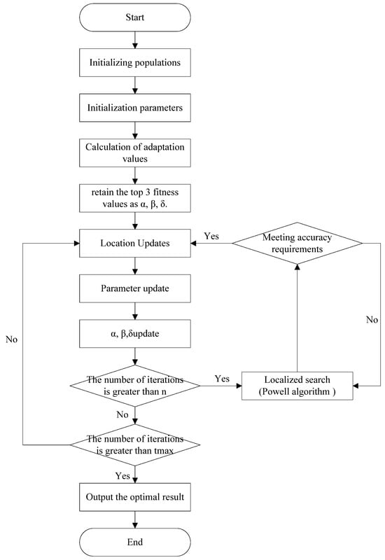
Figure 4.
The computational flow of the PGWO algorithm.
4. Simulation Comparison Experiment and Analysis
Firstly, an abbreviated environment map model is established, and the pipeline search is carried out according to the obstacles and starting points set in this paper to verify the usability of the algorithm. Meanwhile, in order to verify the applicability of the algorithm in the automatic arrangement of ship piping, this paper establishes a simulated environment map and applies an algorithm for piping search based on the actual cabin environment of a real ship.
4.1. Abbreviated Environmental Map Model
In order to verify the usability of the PGWO algorithm, a simple environment map model is selected for validation in this paper. The simple environment map simulates a square cabin, which is discretized by the grid method in the three directions of length, width, and height of the cabin. The spatial model was divided into 100 × 100 × 100 grid cells with a side length of 1 using the grid method, totaling 1 million spatial grid cells.
The obstacles of the piping arrangement are firstly arranged in that space. Then according to the obstacle arrangement and grid distribution, the envelope range of the obstacles in X, Y, and Z directions is obtained. The specific obstacle information in the layout space is shown in Table 1.

Table 1.
Coordinate table of obstacle information.
The experimental platform for the algorithms is Windows 10, 16GB RAM, running on a 64-bit system. In this paper, the grey wolf optimization algorithm (GWO) and the improved grey wolf optimization algorithm (PGWO) are selected for comparison. The population size of all algorithms is set to 50, and the number of iterations is set to 200. Experiments are conducted using Matlab 2021a.
After the experiment, it is found that if the weight of each sub-objective function is set to 1, it is easy to see the situation of the path “going diagonal”. Because the path should be shorter and the number of elbows is less, the weights of each sub-objective function should be set to reduce the path length and the number of elbows and increase the weight of orthogonality. So, set the value of the weight coefficients a = 0.85, b = 0.85, c = 2, d = 1, e = 1. The GWO algorithm, PGWO algorithm, and the algorithm in [12] were used to carry out path optimization calculations 30 times, and the calculation data are shown in Table 2. The results show that these three algorithms can obtain better path layout results. The optimal layout obtained by both algorithms is consistent, as shown in Figure 5.
Table 2.
Statistical data of single pipeline results calculated by GWO and PGWO algorithms.
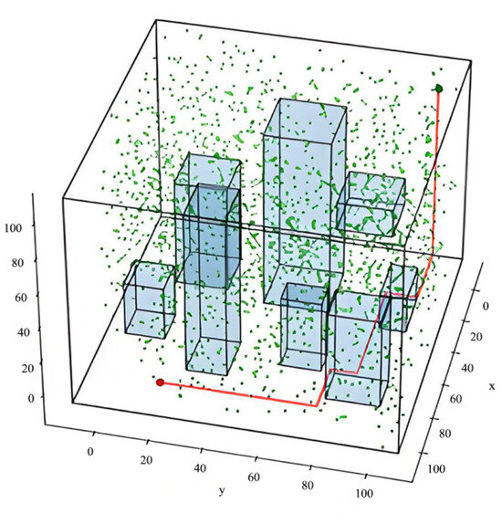
Figure 5.
Layout rendering of single pipeline calculated by GWO and PGWO algorithms.
Firstly, a statistical significance test is performed using a value-of-fitness t-test to verify the performance difference between the GWO and PGWO algorithms. The results are shown in Table 3.
Table 3.
Independent samples test using GWO and PGWO algorithms.
As seen from Table 3, p < 0.05; a significant difference exists between the results of the GWO and PGWO algorithms. Similarly, the PGWO algorithm significantly differs from the algorithm in [12], where Hartley’s isotropic variance test: F = 7891.361, p = 0.000 < 0.05. Similarly, there is a significant difference.
In the respective 30 calculations, the number of optimal layout schemes calculated by the GWO algorithm is 6, and the number of optimal layout schemes obtained by the PGWO algorithm is 25 in terms of the average fitness value and the average number of elbows; compared with the GWO algorithm, the use of the PGWO algorithm reduces the average fitness value and the average number of elbows by 38.03% and 7.69%, respectively. In terms of the average energy zone share, the PGWO algorithm improves the average energy zone share by 20.36%. It can be seen that compared with the GWO algorithm, the PGWO algorithm is more likely to jump out of the local optimization and has a stronger ability to find the global optimization. In addition, the PGWO algorithm has a faster convergence speed, and the average convergence speed can be improved by 36.78% compared with the GWO algorithm. In conclusion, the PGWO algorithm is better than the GWO algorithm in solving the pipe path optimization problem, both in terms of solution quality and convergence speed. In this simulation experiment, the optimal solutions obtained by using the GWO algorithm and the PGWO algorithm are consistent. A comparison of the convergence curves of the optimal solutions obtained from the results of 30 calculations of these two algorithms is shown in Figure 6.
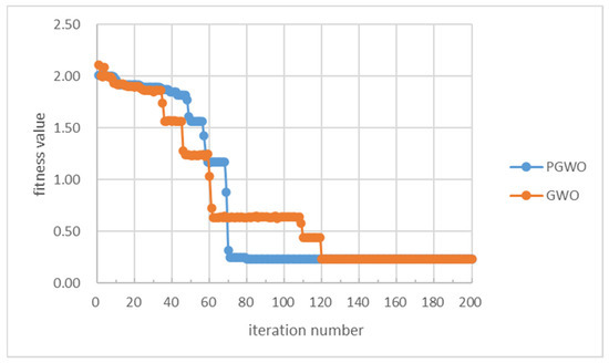
Figure 6.
The convergence curves of the pipeline calculated by GWO and PGWO algorithms.
In the respective 30 calculations, the number of optimal layout schemes calculated by the algorithm in [12] is 16 times. In terms of the average fitness value and the average number of elbows, the use of the PGWO algorithm reduces the average fitness value and the average number of elbows by 30.45% and 7.6%, respectively. In terms of the average energy zone share, the PGWO algorithm improves the average energy zone share by 16.14%. In addition, the PGWO algorithm has a faster convergence speed, and the average convergence speed can be improved by 31.42% compared with the algorithm in [12]. In conclusion, the PGWO algorithm is better than the algorithm in [12] in solving the pipe path optimization problem in terms of solution quality and convergence speed. In this simulation experiment, the optimal solutions obtained by using the algorithm in [12] and the PGWO algorithm are consistent.
4.2. Real Ship Environmental Layout Model
4.2.1. Simple Case Model
Figure 7 shows the cabin structure, and Figure 8 shows the equipment layout space. The system selected is a one-circuit system of filters and bilge pumps, and the equipment consists of filters and bilge pumps.
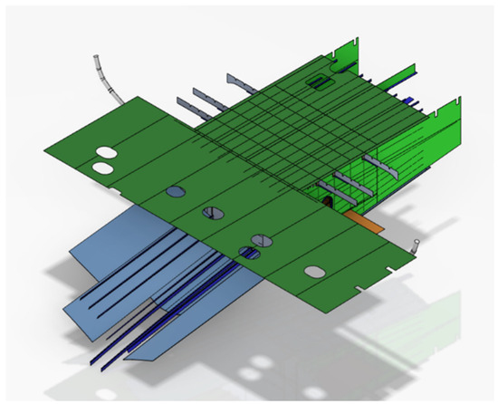
Figure 7.
Cabin structure.
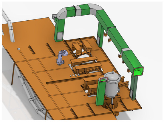
Figure 8.
Equipment layout space.
According to the cabin environment map model, the PGWO algorithm simulates the pipeline search, and Figure 9 shows the optimal calculated 3D pipeline.
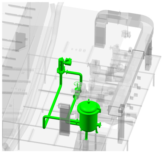
Figure 9.
An optimized pipeline in the ship’s engine room.
From the optimized design results, it can be seen that the design results of the proposed method in this paper meet the engineering design requirements.
4.2.2. Complex Case Model
An example of the piping arrangement in a system compartment is given to test the algorithm’s adaptability and practicality. The example layout space size is 3080 mm × 4860 mm × 2340 mm. The minimum pipe diameter of the pipeline is 100 mm, the grid accuracy is taken as 100 mm, and the layout space is divided into 154 × 243 × 117 cubic grid cells. The interface table (Table 4) gives the equipment connected to the five pipelines, the grid location of the interface point, and the pipe diameter size.
Table 4.
Interface table.
The PGWO algorithm is used to simulate the pipeline search, and the optimal calculated 3D pipeline is shown in Figure 10. The total length of the pipeline is 58,160 mm and the number of elbows is 68.
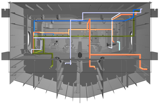
Figure 10.
The optimized layout results.
5. Conclusions
In this paper, we propose to apply the GWO algorithm to pipeline path optimization for the problems of pipeline arrangement in the ship pipeline system. Aiming at the problems of it being easy to fall into the local optimal solution and low computational efficiency when using the GWO algorithm to solve the path optimization problem, a PGWO algorithm is proposed, which uses a nonlinear adaptive convergence strategy in updating the convergence factor, balances the algorithm’s global search and local optimization ability, and mixes the use of Powell’s algorithm, which accelerates the convergence of the algorithm at the later stage.
Simulation results show the following: in dealing with the single-pipe path optimization problem, compared with the GWO algorithm, the PGWO algorithm can improve the computational stability by 63%, and the convergence speed can be improved by 29.18%.
The PGWO algorithm is significantly better than the GWO algorithm both in terms of solution quality and convergence speed. Compared with the traditional piping arrangement method, the piping arrangement using the GWO algorithm can greatly save the design resources, improve the design efficiency, and promote the piping arrangement process in the ship piping system in the direction of intelligence and automation.
Although the method in this paper considers the actual constraints of the ship piping arrangement in the spatial modeling and algorithm design, it still has limitations and is only suitable for solving common cases of the ship piping arrangement. There are many more complex cases to be considered in the actual piping arrangement. For example, for the sake of aesthetics, space-saving, or avoiding liquid accumulation, some pipelines will be arranged in a non-orthogonal form; in order to meet the pipeline function, some pipeline arrangements need to use complex series, parallel, or mixed pipeline network forms. Future work can explore the solution method of complex piping arrangement situations in depth.
The automatic ship piping arrangement method in the paper is only suitable for solving the ship piping arrangement in a narrow sense. In actual ships, there are a large number of cables, heating and ventilation ducts, aisles, and stairs between cabins, and the arrangement of these components belongs to the path planning problem in the broad sense. Subsequent research can combine the domain characteristics of the arrangement problem to extend or modify the existing method to develop a piping arrangement method suitable for other domain applications.
Ship piping arrangement is often limited by the cabin equipment arrangement; the piping arrangement method proposed in this paper is carried out under the premise that the position of the equipment has been fixed, and subsequent research can try to join the piping with the weakly constrained position of the relevant equipment so that the equipment in the space and the piping together achieve the overall optimization of the arrangement.
Automated piping layout methods rely on stochastic strategies that produce different optimization results after different runs. Although these results satisfy the piping arrangement constraints and the evaluation function values of the results are the same or close to each other, they may differ greatly in terms of the actual arrangement effect, and it is necessary to further screen or optimize the combination of the arrangement results by combining them with manual experience. Subsequent research can create a set of evaluation systems for the quality of ship piping arrangement and develop a corresponding intelligent system to automatically evaluate and select the piping arrangement results.
Author Contributions
Y.L.: Conceptualization, Methodology; K.L.: Software, Writing—original raft preparation; R.L.: Data curation, Investigation. Y.W.: Visualization. H.H.: Supervision, Validation. All authors have read and agreed to the published version of the manuscript.
Funding
The author(s) disclosed receipt of the following financial support for the research, authorship, and/or publication of this article: This work was supported by the National Ministry fund project (Grant No. JCKY2021206B009).
Institutional Review Board Statement
Not applicable.
Informed Consent Statement
Not applicable.
Data Availability Statement
No new data were created or analyzed in this study. Data sharing is not applicable to this article.
Conflicts of Interest
The authors declared no potential conflicts of interest with respect to the research, authorship, and/or publication of this article.
References
- Asmara, A. Pipe routing Framework for Detailed Ship Design. Ph.D. Thesis, Delft University of Technology, Delft, The Netherlands, 2013. [Google Scholar]
- Lee, C.Y. An algorithm for path commections and its applications. IRE Trans. Electron. Comput. 1961, EC-10, 346–365. [Google Scholar] [CrossRef]
- Hightower, D.W. A solution to theLine Routing Problem on the Continuous Plane. In Proceedings of the 6th Design Automation Workshop, Miami Beach, FL, USA, 8–12 June 1969; pp. 1–24. [Google Scholar]
- Lu, H.B.; Yu, Z.F.; Sun, P. Hanging bridgealgorithm for Pipe Routing design in ship engine room. In Proceedings of the 2008 International Conference on Computer Science and Software Engineering, Piscataway, NJ, USA, 12–14 December 2008; pp. 153–155. [Google Scholar]
- Bian, X.Y.; Lin, Y.; Dong, Z.R. Auto-routingmethods for complex ship pipe route design. J. Ship Prod. Des. 2022, 38, 100–114. [Google Scholar] [CrossRef]
- Burdorf, A.; Kampczyk, B.; Lederhose, M.; Schmidt-Traub, H. CAPD-computer-aided plant design. Comput. Chem. Eng. 2004, 28, 73–81. [Google Scholar] [CrossRef]
- Kaniat, A. Optimization of three-dimensional piperouting. Ship Technol. Res. 2000, 47, 111–114. [Google Scholar]
- Ren, T.; Zhu, Z.L.; Dimirovski, G.M.; Gao, Z.H.; Sun, X.H.; Yu, H. A new pipe routing method for aero-enginesbased on genetic algorithm. Proc. Inst. Mech. Eng. Part G J. Ofaerospace Eng. 2014, 228, 424–434. [Google Scholar] [CrossRef]
- Wang, H.; Zhao, C.; Yan, W.; Feng, X. Three-Dimensional Multi-Pipe Route Optimization Based on Genetic Algorithms. In Knowledge Enterprise: Intelligent Strategies in Product Design, Manufacturing, and Management, Proceedings of the PROLAMAT 2006, IFIP TC5 International Conference, Shanghai, China, 15–17 June 2006; Springer: Boston, MA, USA, 2006. [Google Scholar]
- Furuholmen, M.; Glette, K.; Hovin, M.; Torresen, J. Evolutionary approaches to the three-dimensionalmulti-pipe routing problem: A comparative study using direct encodings. In Evolutionary Computation in Combinatorial Optimization. EvoCOP 2010; Lecture Notes Incomputer Science; Springer: Boston, MA, USA, 2010; pp. 71–82. [Google Scholar]
- Niu, W.T.; Sui, H.T.; Niu, Y.X.; Cai, K.; Gao, W. Shippipe routing design using NSGA-Il and coevolutionary algorithm. Math. Probl. Eng. 2016, 2016, 7912863. [Google Scholar] [CrossRef]
- Dong, Z.R.; Lin, Y. A particle swarm optimization based approach for ship pipe route design. Int. Shipbuild. Prog. 2017, 63, 59–84. [Google Scholar] [CrossRef]
- Wang, Y.L.; Yu, Y.Y.; Li, K.; Zhao, X.G.; Guan, G. A human computer cooperation improved ant colony optimization for ship pipe route design. Ocean. Eng. 2018, 150, 12–20. [Google Scholar] [CrossRef]
- Wang, C.E.; Liu, Q. Projection and geodesic-based pipe routing algorithm. IEEE Trans. Autom. Sci. Eng. 2011, 8, 641–645. [Google Scholar] [CrossRef]
- Lin, Y.; Bian, X.Y.; Dong, Z.R. A discrete hybrid algorithm based on differential evolution and cuckoo search for optimizing the layout of ship pipe route. Ocean. Eng. 2022, 261, 112–164. [Google Scholar] [CrossRef]
- Jiang, W.Y.; Lin, Y.; Chen, M.; Yu, Y.Y. A co-evolutionaryimproved multi-ant colony optimization for ship multiple and branch pipe route design. Ocean. Eng. 2015, 102, 63–70. [Google Scholar] [CrossRef]
- Sui, H.T.; Niu, W.T. Branch-pipe-routing approach for ship using improved geneticalgorithm. Front. Mech. Eng. 2016, 11, 316–323. [Google Scholar] [CrossRef]
- Dong, Z.R.; Bian, X.Y. Ship pipe route design using improved A* algorithm and genetic algorithm. IEEE Access 2020, 8, 153273–153296. [Google Scholar] [CrossRef]
- Mirjalili, S.; Mirjalili, S.M.; Lewis, A. Grey Wolf Optimizer. Adv. Eng. Softw. 2014, 69, 46–61. [Google Scholar] [CrossRef]
- Engelbrecht, A.P. Fundamentals of Computational Swarm Intelligence; John Wiley & Sons: Hoboken, NJ, USA, 2006. [Google Scholar]
- Tsai, P.W.; Nguyen, T.T.; Dao, T.K. Robot path planning optimization based on multi objective grey wolf optimizer. In Proceedings of the International Conference on Genetic and Evolutionary Computing, Fuzhou, China, 7–9 November 2016; pp. 166–173. [Google Scholar]
- Zhang, S.; Zhou, Y.; Li, Z.; Pan, W. Grey wolf optimizer for unmanned combat aerial vehicle path planning. Adv. Eng. Softw. 2016, 99, 121–136. [Google Scholar] [CrossRef]
- Dewangan, R.K.; Shukla, A.; Godfrey, W.W. Three dimensional path planning using Grey wolf optimizer for UAVs. Appl. Intell. 2019, 49, 2201–2217. [Google Scholar] [CrossRef]
- Radmanesh, M.; Kumar, M.; Sarim, M. Grey wolf optimization based sense and avoidalgorithm in a Bayesian framework for multiple UAV path planning in an uncertain environment. Aerosp. Sci. Technol. 2018, 77, 168–179. [Google Scholar] [CrossRef]
- Wang, X.; Zhao, H.; Han, T.; Zhou, H.; Li, C. A grey wolf optimizer using Gaussian estimation of distribution and its application in the multi-UAV multi-target urban tracking problem. Appl. Soft Comput. 2019, 78, 240–260. [Google Scholar] [CrossRef]
- Powell, M.J.D. An efficient method for finding the minimum of a function of several variables without calculating derivatives. Comput. J. 1964, 7, 155–162. [Google Scholar] [CrossRef]
- Howden, W.E. Reliability of the Path Analysis Testing Strategy. IEEE Trans. Softw. Eng. 2006, SE-2, 208–215. [Google Scholar]
Disclaimer/Publisher’s Note: The statements, opinions and data contained in all publications are solely those of the individual author(s) and contributor(s) and not of MDPI and/or the editor(s). MDPI and/or the editor(s) disclaim responsibility for any injury to people or property resulting from any ideas, methods, instructions or products referred to in the content. |
© 2024 by the authors. Licensee MDPI, Basel, Switzerland. This article is an open access article distributed under the terms and conditions of the Creative Commons Attribution (CC BY) license (https://creativecommons.org/licenses/by/4.0/).