Underwater Refractive Stereo Vision Measurement and Simulation Imaging Model Based on Optical Path

Abstract

When light passes through air–glass and glass–water interfaces, refraction occurs, which affects the accuracy of stereo vision three-dimensional measurements of underwater targets. To eliminate the impact of refraction, we developed a refractive stereo vision measurement model based on light propagation paths, utilizing the normalized coordinate of the underwater target. This model is rigorous in theory, and easy to understand and apply. Additionally, we established an underwater simulation imaging model based on the principle that light travels the shortest time between two points. Simulation experiments conducted using this imaging model verified the performance of the underwater stereo vision measurement model. The results demonstrate that the accuracy achieved by the new measurement model is comparable to that of the stereo vision measurement model in the air and significantly higher than that of the existing refractive measurement model. This is because the light rays from the camera’s optical center to the refraction point at the air–glass interface do not always intersect. The experiments also indicate that the deviation in the refractive index of water lead to corresponding systematic errors in the measurement results. Therefore, in real underwater measurements, it is crucial to carefully calibrate the refractive index of water and maintain the validity of the calibration results.

1. Introduction

Visual measurement can be used for the navigation, monitoring, and 3D reconstruction of underwater structures and organisms [1,2,3,4,5]. When the target is immersed in the water, the camera is usually in a sealed waterproof housing. The light propagating from the target to the camera will be refracted due the density difference between two contacting media, causing the light to no longer be a straight line. If the imaging model and measurement model based on the straight light in the air are still used, it will lead to inaccurate measurement results [6]. The impact of refraction parameters has been analyzed in detail [7].

In order to compensate for the refraction error, a natural approach is to design a special optical component such as a dome window that cancels out the refraction effect through its special shape [8,9]. However, this method has very strict requirements for the production of optical components, limited by the process, and it is difficult to popularize and apply [10,11].

Correspondingly, the camera is placed in a sealed waterproof housing and the target is photographed through a flat transparent window. This method is more flexible and feasible. There are roughly three types of solutions to the imaging distortion problem caused by the flat refractive surfaces. The first approach is to place two auxiliary calibration grids or a calibration frame in the object space, and use the auxiliary calibration structure to determine the direction of the light before it is incident [12]. This method requires customization of the special calibration grid or frame. The second method is the focal length compensation or refraction absorption, which approximates the pixel offset error caused by refraction as the error caused by lens focal length change or distortion, and eliminates the influence of refraction by calibrating the camera’s lens or distortion parameters [13,14,15]. Since the refractive effect is nonlinear and the magnitude of the refraction error depends on the position of the object and the angle of incidence, these methods can only approximately eliminate the effect [16,17]. The last method is the geometric refraction correction. Through geometric analysis, an underwater refraction imaging model is established to explicitly display the refraction effect, theoretically ensuring the accuracy of the measurement results.

For geometric refraction correction, the complex imaging relationships in underwater scenes can be understood by exploring the calibration methods of underwater cameras, and reliable 3D measurements can be made based on the calibrated underwater cameras [18]. The two-stage underwater camera calibration is a pioneering work [19]. Parameters such as the normal vector of the refraction interface and the distance from the refraction interface to the center of the camera can be calibrated based on the optimization method, but appropriate initial values need to be assigned in advance [20]. The analysis and modeling of imaging processing under multilayer media can be used to calculate the refractive index of each medium, the normal vector of each refraction interface, and the distance of the first refraction interface from the camera center [21]. By utilizing the geometric feature that the two incident light rays entering the stereo camera from the same object are on the same plane, the calibration parameters can also be optimized through 3D point remapping [22]. Different frequencies of light have different refractive indices. The parameters of the underwater camera can be calibrated by calculating the offset of the imaging position of different frequencies of light emitted by a specially designed calibration plate at the same position [23]. However, the calibration plate used in this method is expensive. In addition, underwater camera calibration can also use methods such as perspective center displacement and virtual targets [24,25]. In order to eliminate the measurement error caused by the spherical refraction interface, an underwater calibration algorithm based on an advanced nondominated sorting genetic algorithm is proposed using integrated geometric refraction model, which greatly improves the performance of underwater visual measurement [26].

However, these methods are rarely compatible with popular stereo measurement systems that rely on perspective cameras, which leads to many limitations in practical use. Therefore, in order to measure the 3D shape and deformation of underwater objects, researchers have proposed a flexible and compatible stereo vision measurement model based on the flat refractive geometry [27]. The model has already been used to measure the 3D shape of underwater bridge piers [1]. The method assumes that the extension lines of the light cast by the two cameras will converge at one point, but this assumption is only valid within a small range. Therefore, if this method is used for underwater docking navigation such as immersed tunnel element docking [28] and autonomous underwater vehicles recovery [3,29], there are limitations. As the two underwater structures gradually approach each other, the range occupied by targets in the camera’s field of view will become larger and larger, resulting in large errors in the measurement results of targets at the edge of the field of view.

In order to accurately measure all targets within the field of view, the research on the refractive stereo vision measurement model under the air–glass–water condition was conducted. We established an improved refractive 3D measurement model, which is applicable to objects at any position. In order to verify the measurement model, we also studied the simulation measurement model under the condition of three different media, which can be conveniently used for simulation experiments. The flexibility and accuracy of the established measurement model were verified through experiments.

2. Methods

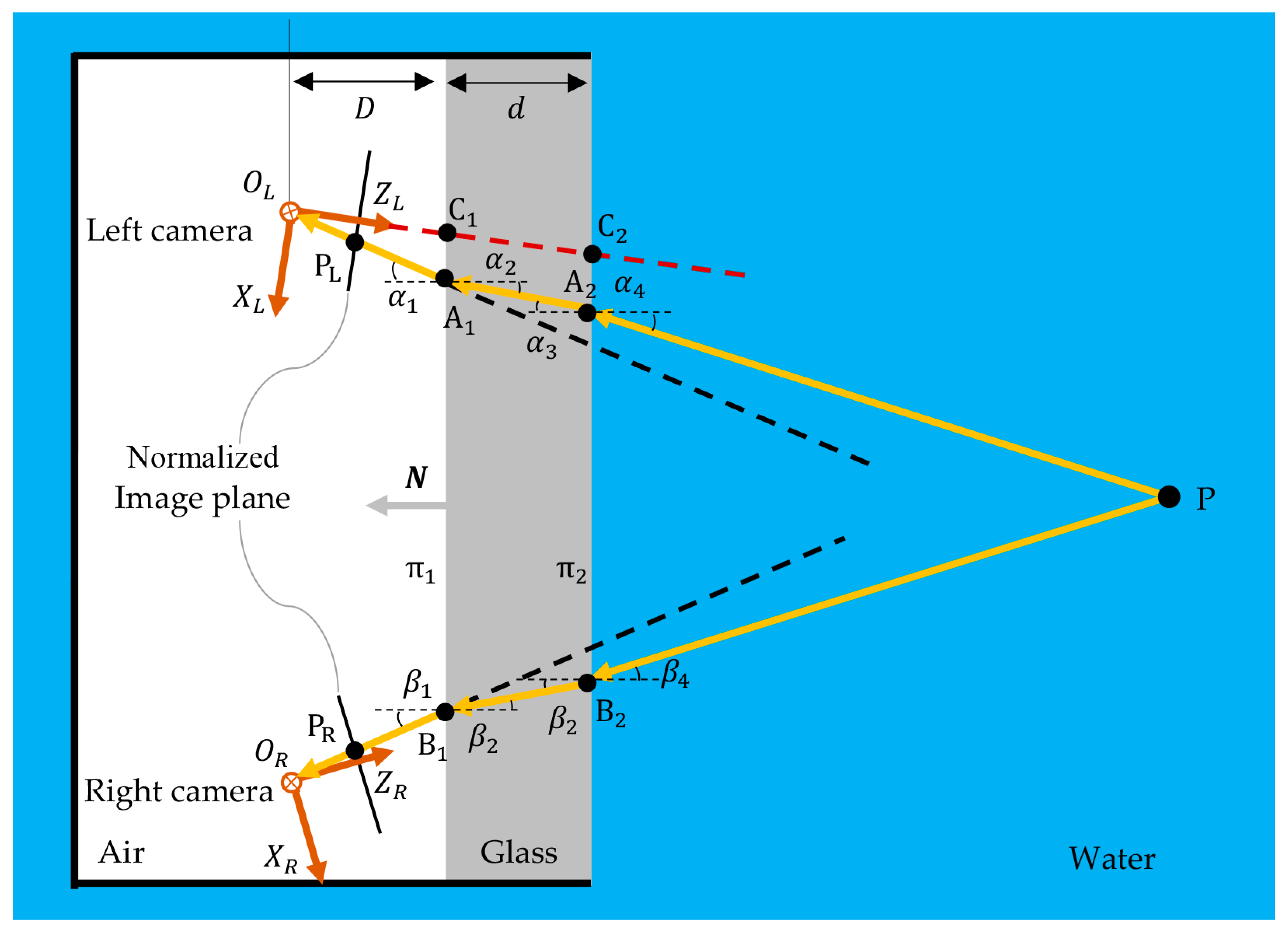
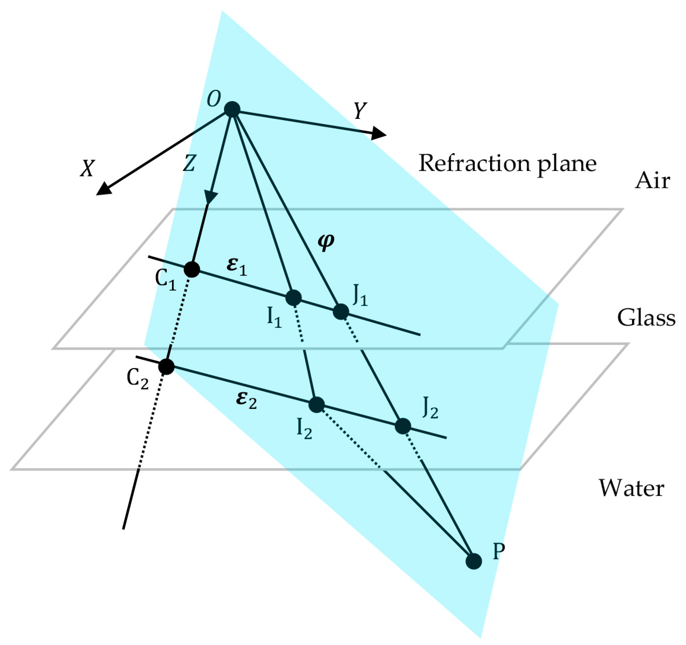
2.1. Stereo Measurement Model with Two Flat Interfaces

The light reflected or emitted by the object in the water passes through the water–glass and glass–air interfaces and reaches the camera in the air. The refracted light rays of stereo vision are shown in Figure 1. Because of the different refractive indices of water, glass, and air, the light from the object P to the left or right camera is not a straight line, but a broken line that is bent at the interface. The light rays from the object to the left and right cameras are $\mathrm{P}{\mathrm{A}}_2$-${\mathrm{A}}_2{\mathrm{A}}_1$-${\mathrm{A}}_1{\mathrm{O}}_{\mathrm{L}}$ and $\mathrm{P}{\mathrm{B}}_2$-${\mathrm{B}}_2{\mathrm{B}}_1$-${\mathrm{B}}_1{\mathrm{O}}_{\mathrm{R}}$, respectively. Let the refractive indices of the air, glass, and water be $n_1$, $n_2$, and $n_3$. The specific values of the refractive indices can be obtained by calibration [27,30,31]. The incidence and refraction angles of the light on the left are ${\alpha }_1$–${\alpha }_4$. The incidence and refraction angles of the light on the right are ${\beta }_1$–${\beta }_4$.

Unlike the assumption in [27], the extension lines of rays ${\mathrm{O}}_{\mathrm{L}}{\mathrm{A}}_1$ and ${\mathrm{O}}_{\mathrm{R}}{\mathrm{B}}_1$ do not necessarily intersect; they may be noncoplanar lines with no intersection. This will be clarified in later experiments. ${\mathrm{P}}_{\mathrm{L}}$ and ${\mathrm{P}}_{\mathrm{R}}$ are the projections of the refraction points ${\mathrm{A}}_1$ and ${\mathrm{B}}_1$ on the normalized plane of the corresponding camera. The three points ${\mathrm{O}}_{\mathrm{L}}$, ${\mathrm{P}}_{\mathrm{L}}$, and ${\mathrm{A}}_1$ are collinear. The three points ${\mathrm{O}}_{\mathrm{R}}$, ${\mathrm{P}}_{\mathrm{R}}$, and ${\mathrm{B}}_1$ are also collinear. The key to calculating the coordinate of point P is to obtain the direction vectors of the refracted light rays ${\mathrm{O}}_{\mathrm{L}}{\mathrm{A}}_1$ and ${\mathrm{O}}_{\mathrm{R}}{\mathrm{B}}_1$.

The camera coordinate systems of the left and right cameras are $O_L-X_L{Y}_L{Z}_L$ and $O_R-X_R{Y}_R{Z}_R$, as shown in Figure 1. $O_L-X_L{Y}_L{Z}_L$ is taken as the reference coordinate system. The rotation matrix of $O_R-X_R{Y}_R{Z}_R$ relative to $O_L-X_L{Y}_L{Z}_L$ is $\mathit{T}$, and the translation vector is $\mathit{t}$. The transformation from the coordinate ${\mathit{X}}_R$ of the right camera coordinate system to the reference coordinate system ${\mathit{X}}_L$ is ${\mathit{X}}_L={\mathit{T}\mathit{X}}_R+\mathit{t}$.

For simplicity, this paper does not consider camera distortion. Two cameras shoot at the same time. After target matching, the left and right camera pixel coordinates ${\mathit{P}}_L^{uv}$ and ${\mathit{P}}_R^{uv}$ of target P are obtained. Therefore, the coordinates of points ${\mathrm{P}}_{\mathrm{L}}$ and ${\mathrm{P}}_{\mathrm{R}}$ on the normalized plane are

$$\left\{\begin{array}{c}{\mathit{P}}_L={\mathit{K}}_L^{-1}{\mathit{P}}_L^{uv}\\ {\mathit{P}}_R=\mathit{T}{\mathit{K}}_R^{-1}{\mathit{P}}_R^{uv}+\mathit{t}\end{array}\right.$$

(1)

where ${\mathit{K}}_L$ and ${\mathit{K}}_R$ are the left and right camera intrinsic matrix; $\mathit{T}$ and $\mathit{t}$ are the rotation matrix and the translation vector of $O_R-X_R{Y}_R{Z}_R$ relative to the reference system. There are mature calibration methods to obtain these camera parameters [32,33].

${\mathit{O}}_L=\left(0,0,0\right)$, ${\mathit{O}}_R=\mathit{t}=\left(t_x,t_y,t_z\right)$. The points ${\mathrm{O}}_{\mathrm{L}}$, ${\mathrm{P}}_{\mathrm{L}}$ and ${\mathrm{A}}_1$ are collinear. The points ${\mathrm{O}}_{\mathrm{R}}$, ${\mathrm{P}}_{\mathrm{R}}$, and ${\mathrm{B}}_1$ are also collinear. Therefore, the unit direction vectors of ${\mathrm{O}}_{\mathrm{L}}{\mathrm{A}}_1$ and ${\mathrm{O}}_{\mathrm{R}}{\mathrm{B}}_1$ can be acquired by

$$\left\{\begin{array}{c}{\mathit{\zeta }}_1={\displaystyle \frac{{\mathit{P}}_L-{\mathit{O}}_L}{\left|{\mathit{P}}_L-{\mathit{O}}_L\right|}}\\ {\mathit{\xi }}_1={\displaystyle \frac{{\mathit{P}}_R-{\mathit{O}}_R}{\left|{\mathit{P}}_R-{\mathit{O}}_R\right|}}\end{array}\right.$$

(2)

where $\left|·\right|$ denotes the vector norm. ${\mathit{\zeta }}_1$ and ${\mathit{\xi }}_1$ are the unit direction vectors of ${\mathrm{O}}_{\mathrm{L}}{\mathrm{A}}_1$ and ${\mathrm{O}}_{\mathrm{R}}{\mathrm{B}}_1$.

The distance $D$ from the left camera to the air–glass interface and the unit normal vector $\mathit{N}$ of the interface can be obtained by calibration [27,30,31]. The unit vector $\mathit{m}$ of $Z_L$-axis of the reference coordinate system is $\left(0,0,1\right)$. Based on $D$ and $\mathit{N}$, the coordinate of the intersection ${\mathrm{C}}_1$ of $Z_L$ axis and the air–glass refraction interface is

$${\mathit{C}}_1=(0,0,{\displaystyle \frac{D}{\mathit{m}·{\mathit{N}}^T}})$$

(3)

If we know the direction vector ${\mathit{v}}_{line}$ of a line and a point ${\mathit{p}}_{line}$ on it, and the normal vector ${\mathit{v}}_{plane}$ of a plane and a point ${\mathit{p}}_{plane}$ on it, then the coordinate of the intersection $\mathrm{p}$ of the line and the plane is

$$\left\{\begin{array}{c}h={\displaystyle \frac{{\mathit{v}}_{plane}·\left({\mathit{p}}_{plane}-{\mathit{p}}_{line}\right)}{{\mathit{v}}_{plane}·{\mathit{v}}_{line}}}\\ \mathit{p}={\mathit{p}}_{line}+h{\mathit{v}}_{line}\end{array}\right.$$

(4)

where $·$ denotes vector dot product.

The direction vector of line ${\mathrm{O}}_{\mathrm{L}}{\mathrm{A}}_1$ and a point on it are ${\mathit{\zeta }}_1$ and ${\mathit{O}}_L$. The direction vector of line ${\mathrm{O}}_{\mathrm{R}}{\mathrm{B}}_1$ and a point on it are ${\mathit{\xi }}_1$ and ${\mathit{O}}_R$. The normal vector to the air–glass interface is $\mathit{N}$, and ${\mathit{C}}_1$ is a point on this plane. Substituting these parameters into Equation (4), the coordinates of the refraction points ${\mathit{A}}_1$ and ${\mathit{B}}_1$ can be obtained.

Based on ${\mathit{\zeta }}_1$, ${\mathit{\xi }}_1$, and $\mathit{N}$, the angles ${\alpha }_1$ and ${\beta }_1$ are

$$\left\{\begin{array}{c}{\alpha }_1={\mathrm{c}\mathrm{o}\mathrm{s}}^{-1}\left({\mathit{\zeta }}_1·{\mathit{N}}^T\right)\\ {\beta }_1={\mathrm{c}\mathrm{o}\mathrm{s}}^{-1}\left({\mathit{\xi }}_1·{\mathit{N}}^T\right)\end{array}\right.$$

(5)

Based on Snell’s law, the angles ${\alpha }_2$ and ${\beta }_2$ are

$$\left\{\begin{array}{c}{\alpha }_2={\sin }^{-1}\left({\displaystyle \frac{n_1·\sin {\alpha }_1}{n_2}}\right)\\ {\beta }_2={\sin }^{-1}\left({\displaystyle \frac{n_1·\sin {\beta }_1}{n_2}}\right)\end{array}\right.$$

(6)

The air–glass refractive interface ${\mathsf{\pi }}_1$ and the glass–water refractive interface ${\mathsf{\pi }}_2$ are assumed to be parallel. ${\alpha }_2={\alpha }_3$, ${\beta }_2={\beta }_3$.

The unit direction vectors of rays ${\mathrm{A}}_1{\mathrm{A}}_2$ and ${\mathrm{B}}_1{\mathrm{B}}_2$ can be calculated as

$$\left\{\begin{array}{c}{\mathit{\zeta }}_2={\displaystyle \frac{n_1}{n_2}}{\mathit{\zeta }}_1-\left({\displaystyle \frac{n_1}{n_2}}\cos {\alpha }_1-\cos {\alpha }_2\right)\mathit{N}\\ {\mathit{\xi }}_2={\displaystyle \frac{n_1}{n_2}}{\mathit{\xi }}_1-\left({\displaystyle \frac{n_1}{n_2}}\cos {\beta }_1-\cos {\beta }_2\right)\mathit{N}\end{array}\right.$$

(7)

The thickness of the glass layer $d$ can be obtained by calibration [27,30,31]. The coordinate of the intersection ${\mathrm{C}}_2$ of $Z_L$ axis and the glass–water refraction interface is

$${\mathit{C}}_2=(0,0,{\displaystyle \frac{D+d}{\mathit{m}·{\mathit{N}}^T}})$$

(8)

The direction vector of line ${\mathrm{A}}_1{\mathrm{A}}_2$ and a point on it are ${\mathit{\zeta }}_2$ and ${\mathrm{A}}_1$. The direction vector of line ${\mathrm{B}}_1{\mathrm{B}}_2$ and a point on it are ${\mathit{\xi }}_2$ and ${\mathrm{B}}_1$. The normal vector to the glass–water interface is $\mathit{N}$, and ${\mathrm{C}}_2$ is a point on this plane. Substituting these parameters into Equation (4), the coordinates of the refraction points ${\mathrm{A}}_2$ and ${\mathrm{B}}_2$ can be obtained.

Based on Snell’s law, the angles ${\alpha }_4$ and ${\beta }_4$ are

$$\left\{\begin{array}{c}{\alpha }_4={\sin }^{-1}\left({\displaystyle \frac{n_2·\sin {\alpha }_3}{n_3}}\right)\\ {\beta }_4={\sin }^{-1}\left({\displaystyle \frac{n_2·\sin {\beta }_1}{n_3}}\right)\end{array}\right.$$

(9)

The unit direction vectors of rays ${\mathrm{A}}_2\mathrm{P}$ and ${\mathrm{B}}_2\mathrm{P}$ are

$$\left\{\begin{array}{c}{\mathit{\zeta }}_3={\displaystyle \frac{n_2}{n_3}}{\mathit{\zeta }}_2-\left({\displaystyle \frac{n_2}{n_3}}\cos {\alpha }_3-\cos {\alpha }_4\right)\mathit{N}\\ {\mathit{\xi }}_3={\displaystyle \frac{n_2}{n_3}}{\mathit{\xi }}_2-\left({\displaystyle \frac{n_2}{n_3}}\cos {\beta }_3-\cos {\beta }_4\right)\mathit{N}\end{array}\right.$$

(10)

Theoretically, the lines ${\mathrm{A}}_2\mathrm{P}$ and ${\mathrm{B}}_2\mathrm{P}$ intersect at P. However, due to the existence of errors, they are likely to be skew lines and have no intersection. Therefore, it is assumed that the midpoint of the common perpendicular of the two lines is P. The two lines ${\mathrm{A}}_2\mathrm{P}$ and ${\mathrm{B}}_2\mathrm{P}$ are determined as

$$\left\{\begin{array}{c}{\mathit{L}}_1\left(s_1\right)={\mathit{A}}_2+s_1{\mathit{\zeta }}_3\\ {\mathit{L}}_2\left(s_2\right)={\mathit{B}}_2+s_2{\mathit{\xi }}_3\end{array}\right.$$

(11)

where $s_1$ and $s_2$ are coefficients. The endpoints of the common perpendicular should satisfy the following equations

$$\left\{\begin{array}{c}\left({\mathit{L}}_1\left(s_1\right)-{\mathit{L}}_2\left(s_2\right)\right)·{\mathit{\zeta }}_3=0\\ \left({\mathit{L}}_1\left(s_1\right)-{\mathit{L}}_2\left(s_2\right)\right)·{\mathit{\xi }}_3=0\end{array}\right.$$

(12)

In the above equations, only $s_1$ and $s_2$ are unknown. Solving the above equations will give us the values $s_1$ and $s_2$. Assume that the foot of the perpendicular to line ${\mathrm{A}}_2\mathrm{P}$ is point ${\mathrm{P}}_1$, and the foot of the perpendicular to line ${\mathrm{B}}_2\mathrm{P}$ is point ${\mathrm{P}}_2$. Substituting $s_1$ and $s_2$ into Equation (11), we obtain the coordinates of ${\mathrm{P}}_1$ and ${\mathrm{P}}_2$

$$\left\{\begin{array}{c}{\mathit{P}}_1={\mathit{L}}_1\left(s_1\right)\\ {\mathit{P}}_2={\mathit{L}}_2\left(s_2\right)\end{array}\right.$$

(13)

The coordinate of the midpoint P is the average of the coordinates of ${\mathrm{P}}_1$ and ${\mathrm{P}}_2$

$$\mathit{P}={\displaystyle \frac{{\mathit{P}}_1+{\mathit{P}}_2}{2}}$$

(14)

The 3D coordinate of point P is successfully obtained.

2.2. Simulation Imaging Model with Two Flat Interfaces

It is necessary to verify the measurement model through experiments. Real underwater experiments involve a complex environment, making data acquisition difficult, with more sources of error. In contrast, simulation experiments are convenient for artificially controlling the presence and size of errors, and are easy to implement. Therefore, we will use simulation experiments to verify the measurement model. To facilitate the simulation experiment, a simulation imaging model was studied based on the principle that the time it takes for light to propagate between two points is the shortest.

The propagation path of the light from the target to the camera is shown in Figure 2. The origin of the camera coordinate system is O, and its coordinate in the reference coordinate system is $\mathit{O}=\left(X_o,Y_o,Z_o\right)$. The coordinate of the target is $\mathit{P}=\left(X_1,Y_1,Z_1\right)$. The unit normal vector of the refractive interface is N. The refractive indices of air, glass, and water are $n_1$, $n_2$, and $n_3$. The actual optical path between the camera optical center O and the target P is $\mathrm{O}{\mathrm{I}}_1$-${\mathrm{I}}_1{\mathrm{I}}_2$-${\mathrm{I}}_2\mathrm{P}$. ${\mathrm{I}}_1$ and ${\mathrm{I}}_2$ are the points where the light is refracted at the air–glass and glass–water interfaces. ${\mathrm{J}}_1$ and ${\mathrm{J}}_2$ are the intersection points of the line connecting the camera optical center and the target and the two refractive interfaces. The actual optical path and the line connecting the camera optical center and the target lie in the refraction plane [21]. The primary goal of the simulation is to calculate the coordinate of point ${\mathrm{I}}_1$ based on the coordinates of points O and P. Once the coordinate of point ${\mathrm{I}}_1$ is known, the pixel coordinate corresponding to target P can be simulated using the perspective imaging model.

The unit direction vector of line OP is

$$\mathit{\phi }={\displaystyle \frac{\mathit{P}-\mathit{O}}{\left|\mathit{P}-\mathit{O}\right|}}$$

(15)

Since $\mathrm{O}{\mathrm{I}}_1$, ${\mathrm{I}}_1{\mathrm{I}}_2$, and ${\mathrm{I}}_2\mathrm{P}$ are coplanar with the normal vector, $\mathit{N}$, of the refraction interfaces, the unit normal vector of the refraction plane is

$$\mathit{\chi }={\displaystyle \frac{\mathit{\phi }\times \mathit{N}}{‖\mathit{\phi }\times \mathit{N}‖}}$$

(16)

where $\times$ denotes the cross-product. The unit direction vector of the intersection line ${\mathrm{I}}_1{\mathrm{J}}_1$ of the refraction plane and the air–glass interface is

$${\mathit{\epsilon }}_1={\displaystyle \frac{\mathit{\chi }\times \mathit{N}}{‖\mathit{\chi }\times \mathit{N}‖}}$$

(17)

In real underwater experiments or practical applications, the distance $D$ from the origin of the reference coordinate system to the air–glass interface, the thickness of the glass layer $d$, the unit normal vector $\mathit{N}$ of the refractive interface, and the refractive indices can be calibrated [27,30,31]. In simulation experiments, these parameters can be specified manually.

Using Equation (3), we can obtain the coordinate of the intersection point ${\mathrm{C}}_1$ of the $Z$ axis and the air–glass interface. The direction vector of line $\mathrm{O}\mathrm{P}$ and a point on it are $\mathit{\phi }$ and $\mathrm{O}$. The normal vector to the air–glass interface is $\mathit{N}$, and ${\mathrm{C}}_1$ is a point on this plane. Substituting these parameters into Equation (4), the coordinates of the intersection point ${\mathrm{J}}_1$ can be obtained. Then, the line ${\mathrm{I}}_1{\mathrm{J}}_1$ can be expressed as

$${\mathit{r}}_1\left({\mu }_1\right)={\mathit{J}}_1+{\mu }_1{\mathit{\epsilon }}_1$$

(18)

where ${\mu }_1$ is the coefficient.

Similarly, using Equation (8), we can obtain the coordinate ${\mathit{C}}_2$ of the intersection of the $Z$ axis and the glass–water interface. The direction vector of line $\mathrm{O}\mathrm{P}$ and a point on it are $\mathit{\phi }$ and $\mathrm{O}$. The normal vector to the glass–water interface is $\mathit{N}$, and ${\mathrm{C}}_2$ is a point on this plane. Substituting these parameters into Equation (4), the coordinates of the intersection point ${\mathrm{J}}_2$ can be obtained. Then, the line ${\mathrm{I}}_2{\mathrm{J}}_2$ can be expressed as

$${\mathit{r}}_2\left({\mu }_2\right)={\mathit{J}}_2+{\mu }_2{\mathit{\epsilon }}_2$$

(19)

where ${\mu }_2$ is the coefficient.

According to the relationship between refractive index and the speed of light, if the speed of light in vacuum is c, the speeds of light in the air, glass and water are

$$\left\{\begin{array}{c}{v}_a={\displaystyle \frac{c}{n_1}}\\ v_g={\displaystyle \frac{c}{n_2}}\\ v_w={\displaystyle \frac{c}{n_3}}\end{array}\right.$$

(20)

Therefore, the actual propagation time of light from the target P to the optical center O is

$$t={\displaystyle \frac{\left|{\mathit{I}}_1-\mathit{O}\right|}{v_a}}+{\displaystyle \frac{\left|{\mathit{I}}_2-{\mathit{I}}_1\right|}{v_g}}+{\displaystyle \frac{\left|\mathit{P}-{\mathit{I}}_2\right|}{v_w}}$$

(21)

${\mathrm{I}}_1$ and ${\mathrm{I}}_2$ are points on lines ${\mathrm{I}}_1{\mathrm{J}}_1$ and ${\mathrm{I}}_2{\mathrm{J}}_2$ respectively. Hence,

$$\left\{\begin{array}{c}{\mathit{I}}_1={\mathit{r}}_1\left({\mu }_1\right)\\ {\mathit{I}}_2={\mathit{r}}_2\left({\mu }_2\right)\end{array}\right.$$

(22)

Substituting Equation (22) into (21), we can obtain the function $t$ with respect to ${\mu }_1$ and ${\mu }_2$. $t=f\left({\mu }_1,{\mu }_2\right)$. According to Fermat’s principle, the time it takes for light to travel between two points is the shortest. Therefore, we need to find ${\mu }_1$ and ${\mu }_2$ at the minimum value of function $t$. First, we construct a system of equations in which the partial derivatives of $t$ with respect to ${\mu }_1$ and ${\mu }_2$ are 0.

$$\left\{\begin{array}{c}{\displaystyle \frac{\partial t}{\partial \left({\mu }_1\right)}}=0\\ {\displaystyle \frac{\partial t}{\partial \left({\mu }_2\right)}}=0\end{array}\right.$$

(23)

Solving this system of equations, we can obtain the critical point $\left({\mu }_1,{\mu }_2\right)$. Then, we calculate the second-order partial derivatives and construct the Hessian matrix $\mathit{H}$.

$$\mathit{H}=\left(\begin{array}{cc}{\displaystyle \frac{{\partial }^{2}t}{\partial \left({\mu }_1^2\right)}}& {\displaystyle \frac{{\partial }^{2}t}{\partial \left({\mu }_1\right)\partial \left({\mu }_2\right)}}\\ {\displaystyle \frac{{\partial }^{2}t}{\partial \left({\mu }_2\right)\partial \left({\mu }_1\right)}}& {\displaystyle \frac{{\partial }^{2}t}{\partial \left({\mu }_2^2\right)}}\end{array}\right)$$

(24)

If the following holds

$$\mathrm{d}\mathrm{e}\mathrm{t}\left(\mathit{H}\right)>0 \mathrm{a}\mathrm{n}\mathrm{d} {\displaystyle \frac{{\partial }^{2}t}{\partial \left({\mu }_1^2\right)}}>0$$

(25)

where $\mathrm{d}\mathrm{e}\mathrm{t}\left(\mathit{H}\right)$ denotes the determinant of matrix $\mathit{H}$. Then $\left({\mu }_1,{\mu }_2\right)$ is a minimum value. Substituting $\left({\mu }_1,{\mu }_2\right)$ into Equation (22) we can obtain the refraction points ${\mathrm{I}}_1$ and ${\mathrm{I}}_2$.

Under air–glass–water conditions, the camera’s imaging of a target P in the water is the same as its imaging of point ${\mathrm{I}}_1$ at the air–glass interface. The target pixel coordinate can be readily determined using the perspective imaging model by utilizing the coordinate ${\mathit{I}}_1$ and the camera parameters, thereby enabling the simulation of the imaging process.

3. Results

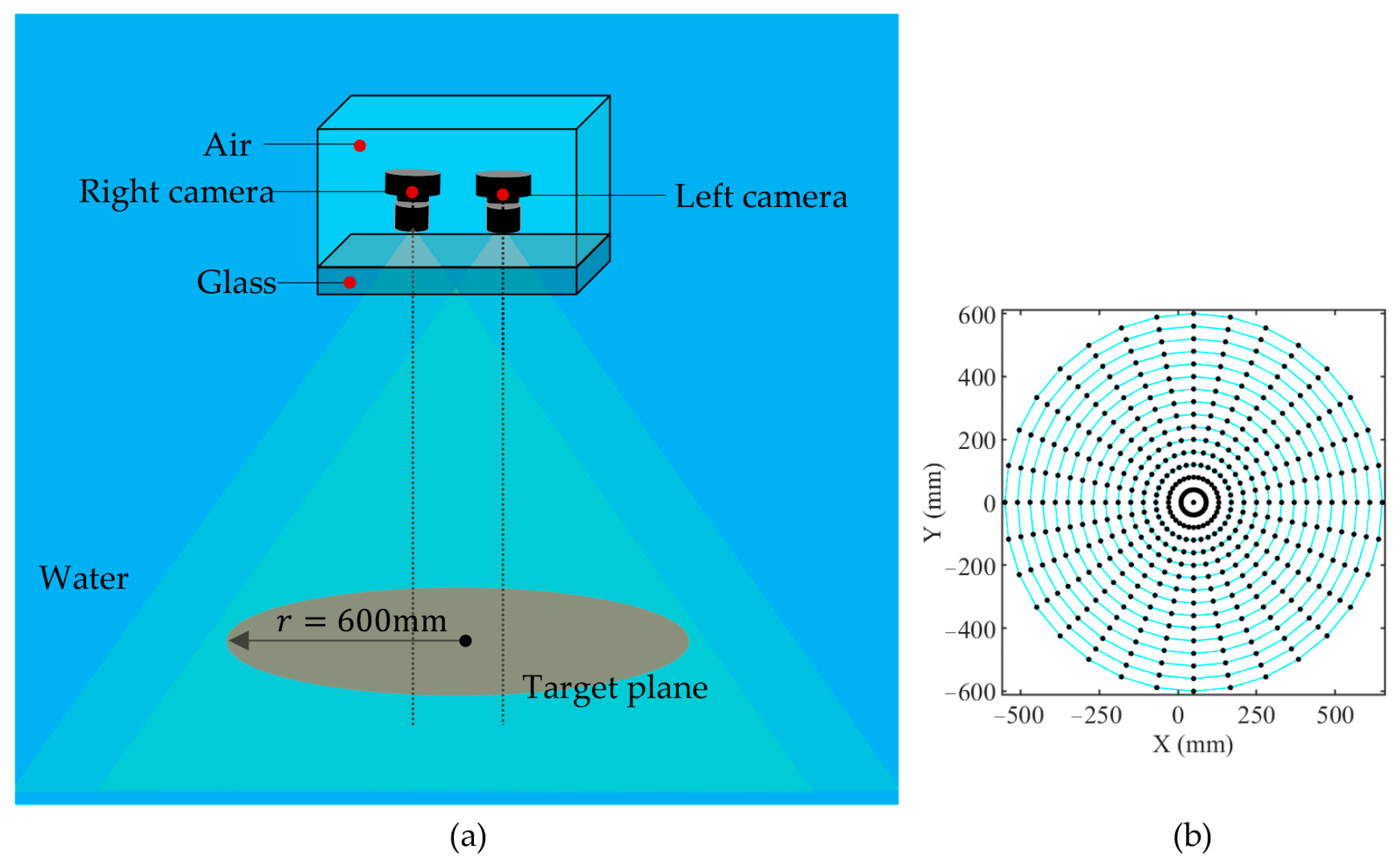
3.1. Experimental Design

In order to better verify and evaluate the performance of the stereo measurement model, simulation experiments based on the proposed simulation imaging model were conducted, which can avoid the interference of other errors as much as possible. The experimental settings are shown in Figure 3. The two cameras are placed in a housing. The sealed housing and the targets are submerged in water. The cameras can image the targets through a glass window. The window is flat, with two surfaces parallel to each other. All the targets are on a same plane and in the public view of both cameras. The target plane is a circular area with radius of 600 mm. Fifteen concentric circles with different radii are set in the target region. A total of 33 points are evenly selected on each circle, and the radius difference of adjacent circles is equal. There are a total of 496 points, each with known coordinates in the reference coordinate system.

The intrinsic and external parameters of the cameras were obtained by calibration [32,33]. The distance $D$ of the left camera from the air–glass surface, the glass thickness $d$, the unit normal $\mathit{N}$ of the refraction interfaces, and the refraction indices $n_1$, $n_2$, and $n_3$ were artificially assigned, as shown in

Table 1. The refraction parameters assigned in the simulation experiments.

$\mathit{D}$ (mm)	$\mathit{d}$ (mm)	$\mathit{N}$	${\mathit{n}}_1$	${\mathit{n}}_2$	${\mathit{n}}_3$
100	5	$\left(0,0,1\right)$	1	1.54	1.33

. In real underwater experiments or practical applications, the refraction parameters can be obtained through calibration [27,30,31].

3.2. Intersection of Refracted Light from the Left and Right Cameras

The purpose of this experiment is to evaluate whether and to what extent the extension lines of rays ${\mathrm{O}}_{\mathrm{L}}{\mathrm{A}}_1$ and ${\mathrm{O}}_{\mathrm{R}}{\mathrm{B}}_1$ in Figure 1 intersect. The target plane is 1 m away from the left camera. In this setting, the target plane almost fills the camera’s field of view. Using Snell’s law, the error-free coordinates of refraction points, ${\mathit{A}}_1$ and ${\mathit{B}}_1$, as shown in Figure 1, and pixel coordinates corresponding to each point, P, were simulated using the simulation imaging model in Section 2.2.

According to Equations (1) and (2), the direction vectors of the two refracted rays ${\mathrm{O}}_{\mathrm{L}}{\mathrm{A}}_1$ and ${\mathrm{O}}_{\mathrm{R}}{\mathrm{B}}_1$ were calculated. Then, similar to Equations (11)–(13), the foots of the common perpendicular of rays ${\mathrm{O}}_{\mathrm{L}}{\mathrm{A}}_1$ and ${\mathrm{O}}_{\mathrm{R}}{\mathrm{B}}_1$ were calculated. Finally, the length of the common perpendicular was calculated, which was the shortest distance between the two rays. The shortest distance is used to determine whether the two rays intersect.

The results are shown in Figure 4. It can be clearly seen that in the circular area with a radius of 600 mm and a distance of 1 m from the left camera, the length of the common perpendicular of the refracted light rays corresponding to most objects is greater than 0.6 mm, indicating that the refracted light rays ${\mathrm{O}}_{\mathrm{L}}{\mathrm{A}}_1$ and ${\mathrm{O}}_{\mathrm{R}}{\mathrm{B}}_1$ do not always intersect in theory. The shape of the contour is a four-pointed star, and the closer to the center of the area, the smaller the length of the common perpendicular. If the shortest distance between two straight lines is greater than ${10}^{-6} \mathrm{m}\mathrm{m}$ as the criterion for judging whether the straight lines intersect, then among all 496 objects, the refracted light rays corresponding to more than 90% of the objects do not intersect. Therefore, the method of obtaining the virtual target point through triangulation and then calculating the direction vectors of the refracted light rays ${\mathrm{O}}_{\mathrm{L}}{\mathrm{A}}_1$ and ${\mathrm{O}}_{\mathrm{R}}{\mathrm{B}}_1$ is only effective for targets within a very small range in the center of the field of view. Applying it to all objects in the field of view would artificially introduce model errors. This proves the necessity of the new refractive measurement model proposed in Section 2.1.

3.3. Performance Evaluation of Stereo Measurement Model

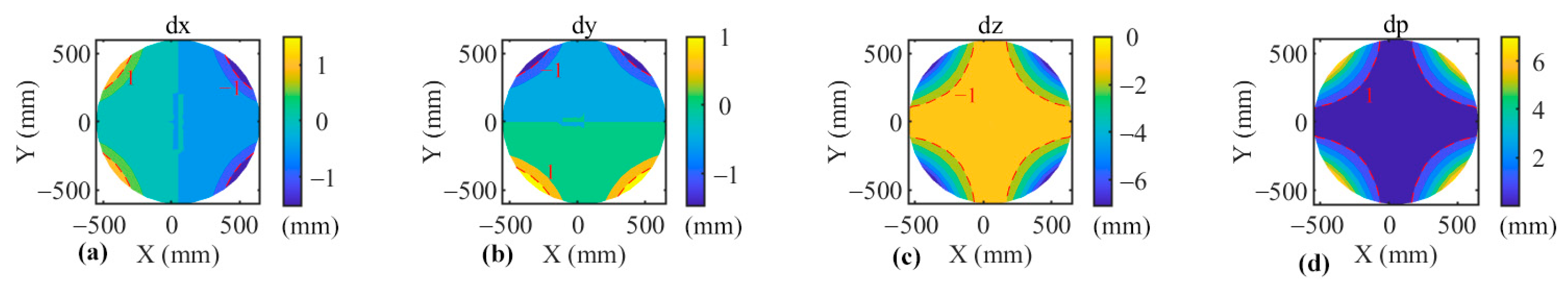
3.3.1. Ideal Conditions

First, the performance of the stereo vision measurement model and the simulation model is evaluated under ideal conditions. The experimental settings are the same as in Section 3.1. All coordinates and parameters are error-free and bias-free. The target plane is set to be 1 m away from the left camera. For comparison, we also carried out the simulation experiment in the air, and the experimental settings in the air were unchanged except for single-medium measurements. In the single air scene, the pixel coordinate corresponding to each object point was simulated using the perspective imaging model. Based on Snell’s law, the error-free refraction points and pixel coordinate of each object were obtained using the simulation imaging model.

Based on the pixel coordinates obtained by simulation, the coordinates of objects are estimated using three measurement models. The first model is the model proposed in Section 2.1. The second model is the model established in [27], which is called Su’s method. The third model is the regular triangulation used in the air, which is called the regular method. Three kinds of coordinates are obtained, and then the discrepancy between the measured coordinate and the true coordinate is calculated:

$$\left\{\begin{array}{c}{d}_x=X_m-X_t\\ d_y=Y_m-Y_t\\ d_z=Z_m-Z_t\\ d_P=\sqrt{d_x^2+d_y^2+d_z^2}\end{array}\right.$$

(26)

where $\left(X_m,Y_m,Z_m\right)$ is the measured coordinate, and $\left(X_t,Y_t,Z_t\right)$ is the true coordinate.

The deviations obtained by both our method and the regular method are in the order of ${10}^{-11}$ mm, and their distribution within the field of view appears random, suggesting that they are caused by numerical errors. This indicates that the simulation model and measurement model proposed in Section 2 are themselves free of error. When the camera parameters and refraction parameters are error-free, our new model can obtain results consistent with the true value, just like the conventional stereoscopic vision measurement model in the air. The results obtained by Su’s model are shown in Figure 5. In contrast, the coordinate deviation obtained by Su’s model is related to the distribution of the target. The coordinate of the target close to the center of the field of view is close to their true value, but the coordinate of the target at the edge of the field of view deviates from their true value by a large margin. The maximum $d_P$ exceeds 50 mm.

In order to further analyze the performance of the underwater 3D measurement model, the distance from the target plane to the left camera was increased to 2 m, and the similar simulation was performed. The discrepancy of the results obtained by our new method and the regular method is maintained at the order of ${10}^{-10}$ or ${10}^{-11}$ mm. It is considered that the measured coordinates are consistent with the true values, and there is no error in the model itself. The results of Su’s method are shown in Figure 6. The results of Su’s method are improved, but the maximum $d_P$ is still more than 7 mm. However, compared with Figure 5, the coordinate deviation obtained by Su’s model is significantly reduced. The range of the $\pm 1$ mm contour line has become significantly larger. This is because as the distance from the target plane to the left camera increases, the range of the target area in the field of view becomes smaller. This shows that the new method is not affected by the object position and can always obtain high-quality measurement results, and Su’s method has good performance for objects near the center area.

3.3.2. Simulated Pixel Coordinates Containing Errors

In practical applications, the matched pixel coordinates will inevitably contain errors. Therefore, Gaussian noise (variance 0.01 pixel) is artificially added to the simulated pixel coordinates to evaluate the performance of the underwater stereo vision measurement model [34]. The experimental settings are the same as in Section 3.1. The target plane is 1 m away from the left camera. Refraction parameters contain no errors. Similar to Section 3.3.1, simulation experiments were carried out using our, Su’s, and the regular models in the air to calculate the target’s coordinate deviation.

The results are shown in Figure 7. The deviation in coordinates obtained by our model and the regular model reaches the millimeter level when pixel coordinates contain errors. The deviation in the X-coordinate was minimal, generally within ±1 mm, while the deviation in the Z-coordinate was the largest, exceeding ±2 mm. And the deviation was independent of the target’s distribution, exhibiting randomness within the target area. Our method even outperforms the regular model in the air, with the deviations of the X, Y, and total coordinates obtained by our new method being minimal. The deviation in coordinates obtained by Su’s model closely aligns with the results shown in Figure 5, indicating that even in the presence of Gaussian noise (variance 0.01 pixel) in pixel coordinates, the results from Su’s model are still primarily influenced by model error.

The normalized histograms of coordinate deviations obtained by our model and Su’s model and the fitted Gaussian curves are shown in Figure 8. The means of the three types of coordinate deviations obtained by our model are all close to 0, and the histograms are symmetrically distributed. The X and Y coordinate deviations obtained by Su’s model are also close to 0, and the histograms are symmetrically distributed, but the Z coordinate deviations are all negative. This shows that the results obtained by our model show randomness under the influence of pixel coordinate errors, while the model error of Su’s method introduces systematic deviations to the Z coordinate.

3.3.3. Simulated Pixel Coordinates with Errors and n₃ with Deviation

Furthermore, in practical applications, in addition to the errors in pixel coordinates, the calibration of refraction parameters must contain measurement errors, resulting in deviations between the calibrated refraction parameters and their true values. Among all the refraction parameters, the distance from the air–glass interface to the camera, the thickness of the glass layer, the normal vector of the refraction interface, and the refractive indices of air and glass can all be fixed and remain unchanged, so accurate results can be obtained through rigorous calibration. Water is more complex, and the refractive index of different waters may be different [35]. Although the water refractive index deviation obtained by calibration can be controlled within 0.15% [30], the impact of this deviation is also worth analyzing. Therefore, in this experiment, Gaussian noise (variance 0.01 pixel) is artificially added to the pixel coordinates, and a 0.15% deviation is added to the refractive index of water to evaluate the performance of the underwater stereo vision measurement model. The experimental setting is the same as described in Section 3.1. The target plane is 1 m away from the left camera. The simulation experiment is conducted using both our new model and Su’s model. The coordinate deviation of the target is calculated.

The results are shown in Figure 9. Compared with Figure 7, the coordinate deviations obtained by our model have slightly increased. Both the X and Z coordinate deviations have moved in the negative direction, which means that when the refractive index of water contains the deviation, the results obtained by our model, especially the X and Z coordinates, will have small systematic errors. Compared with Figure 7, the coordinate deviation obtained by Su’s model is basically unchanged.

The normalized histograms of the coordinate deviations and the Gaussian curves obtained by fitting are shown in Figure 10. Compared with Figure 8, the distribution of the Y coordinate deviation obtained by our model has not changed, while the mean values of the X and Z coordinate deviations have changed in the negative direction. The distribution of the Y coordinate deviation obtained by Su’s model has basically not changed, and the mean values of the X and Z coordinate deviations have also changed in the negative direction, and the magnitude of the change is the same as the result of our model. This shows that the refractive index deviation of water has a similar effect on the two models.

4. Discussion

A flexible and easy-to-use underwater stereo vision measurement model applicable to all targets within the field of view based on the light path is investigated. And a simulation imaging model is established based on the principle that light propagation time between two points is the shortest. The experimental results demonstrate that the simulation imaging model can accurately obtain the pixel coordinates of the target, which is a prerequisite for the smooth progress of the simulation experiments. It is confirmed that the light rays from the camera’s optical center to the refraction points at the air–glass interfaces do not always intersect at a single point. In fact, for most targets within the field of view, these rays do not intersect. The closer the targets are to the edge of the field of view, the farther apart their corresponding refracted rays are. The proposed stereo vision measurement model is constructed according to the light propagation paths and its accuracy is analogous to the regular triangulation used in the air. Theoretically, it is highly rigorous, without model errors. Therefore, the simulation results obtained from the new model are similar to those obtained from the regular measurement models in the air, both exhibiting high accuracy and surpassing the underwater vision measurement model proposed in [27]. The advantages of our model become more pronounced for underwater targets located closer to the edge of the field of view. In addition to the air–glass–water scenario, the stereo vision measurement model and simulation imaging model established in this paper are also applicable to other multimedium scenarios.

Considering the ease of implementation and the advantage of variable control in simulation experiments, this study primarily conducts simulation experiments based on the established simulation imaging model. The experimental results provide guidance for future experiments or practical applications in complex real-world environments. The deviation in the refractive index of water can cause systematic errors in the obtained X and Z coordinates. As environmental factors such as temperature change, the refractive index of water also changes [35]. Therefore, in real underwater experiments and practical applications, attention should be given to the calibration of the water’s refractive index and to ensuring the validity of the calibration results. This also suggests that although there are already numerous methods for calibrating refractive parameters, it is possible in the future to develop measurement models that do not require prior calibration of the water’s refractive index. Instead, the refractive index parameters could be estimated simultaneously during the measurement process, thereby enabling better vision measurements in dynamic water environments.

5. Conclusions

This paper presents an underwater stereo vision measurement model based on the actual light propagation path, with a corresponding simulation imaging model established according to the principle of light propagation. Simulation experiments demonstrate that the proposed new measurement model can achieve results comparable to stereo vision measurements in the air. Compared to the existing underwater vision measurement model, the new model offers higher accuracy, particularly for targets located at the edges of the field of view. The new measurement and simulation imaging models are applicable to multimedium environments, including air–glass–water scenarios. This study underscores the importance of calibrating the refractive index of water in real underwater experiments and practical applications. Additionally, it suggests the potential for developing future measurement models that do not require prior calibration of the water’s refractive index, thereby enabling more accurate vision measurements in dynamic water environments.

References

1. Wu, T.; Hou, S.; Sun, W.; Shi, J.; Yang, F.; Zhang, J.; Wu, G.; He, X. Visual measurement method for three-dimensional shape of underwater bridge piers considering multirefraction correction. Automat. Constr. 2023, 146, 104706. [Google Scholar] [CrossRef]
2. Nocerino, E.; Menna, F.; Gruen, A.; Troyer, M.; Capra, A.; Castagnetti, C.; Rossi, P.; Brooks, A.J.; Schmitt, R.J.; Holbrook, S.J. Coral Reef Monitoring by Scuba Divers Using Underwater Photogrammetry and Geodetic Surveying. Remote Sens. 2020, 12, 3036. [Google Scholar] [CrossRef]
3. Liu, S.; Xu, H.; Lin, Y.; Gao, L. Visual Navigation for Recovering an AUV by Another AUV in Shallow Water. Sensors 2019, 19, 1889. [Google Scholar] [CrossRef]
4. Bruno, F.; Bianco, G.; Muzzupappa, M.; Barone, S.; Razionale, A.V. Experimentation of structured light and stereo vision for underwater 3D reconstruction. ISPRS J. Photogramm. 2011, 66, 508–518. [Google Scholar] [CrossRef]
5. Kazakidi, A.; Zabulis, X.; Tsakiris, D.P. Vision-based 3D motion reconstruction of octopus arm swimming and comparison with an 8-arm underwater robot. In Proceedings of the 2015 IEEE International Conference on Robotics and Automation (ICRA), Seattle, WA, USA, 26–30 May 2015. [Google Scholar]
6. Chadebecq, F.; Vasconcelos, F.; Lacher, R.; Maneas, E.; Desjardins, A.; Ourselin, S.; Vercauteren, T.; Stoyanov, D. Refractive Two-View Reconstruction for Underwater 3D Vision. Int. J. Comput. Vis. 2020, 128, 1101–1117. [Google Scholar] [CrossRef]
7. Tong, Z.; Gu, L.; Shao, X. Refraction error analysis in stereo vision for system parameters optimization. Measurement 2023, 222, 113650. [Google Scholar] [CrossRef]
8. Treibitz, T.; Schechner, Y.Y. Active Polarization Descattering. IEEE Trans. Pattern Anal. Mach. Intell. 2009, 31, 385–399. [Google Scholar] [CrossRef] [PubMed]
9. Schechner, Y.Y.; Karpel, N. Recovery of Underwater Visibility and Structure by Polarization Analysis. IEEE J. Ocean. Eng. 2005, 30, 570–587. [Google Scholar] [CrossRef]
10. Łuczyński, T.; Pfingsthorn, M.; Birk, A. The Pinax-model for accurate and efficient refraction correction of underwater cameras in flat-pane housings. Ocean. Eng. 2017, 133, 9–22. [Google Scholar] [CrossRef]
11. Menna, F.; Nocerino, E.; Fassi, F.; Remondino, F. Geometric and Optic Characterization of a Hemispherical Dome Port for Underwater Photogrammetry. Sensors 2016, 16, 48. [Google Scholar] [CrossRef]
12. Kwon, Y.; Casebolt, J.B. Effects of light refraction on the accuracy of camera calibration and reconstruction in underwater motion analysis. Sport. Biomech. 2006, 5, 95–120. [Google Scholar] [CrossRef] [PubMed]
13. Fabio, M.; Erica, N.; Salvatore, T.; Fabio, R. A photogrammetric approach to survey floating and semi-submerged objects. In Proceedings of the Videometrics, Range Imaging, and Applications XII, and Automated Visual Inspection, Munich, Germany, 13–16 May 2013. [Google Scholar]
14. Kang, L.; Wu, L.; Yang, Y. Experimental study of the influence of refraction on underwater three-dimensional reconstruction using the SVP camera model. Appl. Opt. 2012, 51, 7591–7603. [Google Scholar] [CrossRef]
15. Lavest, J.M.; Rives, G.; Laprest, J.T. Underwater Camera Calibration. In Proceedings of the European Conference on Computer Vision (ECCV) 2000, Dublin, Ireland, 26 June–1 July 2000. [Google Scholar]
16. Treibitz, T.; Schechner, Y.; Kunz, C.; Singh, H. Flat Refractive Geometry. IEEE Trans. Pattern Anal. Mach. Intell. 2012, 34, 51–65. [Google Scholar] [CrossRef]
17. Kang, L.; Wu, L.; Wei, Y.; Lao, S.; Yang, Y. Two-view underwater 3D reconstruction for cameras with unknown poses under flat refractive interfaces. Pattern Recogn. 2017, 69, 251–269. [Google Scholar] [CrossRef]
18. Shortis, M. Calibration Techniques for Accurate Measurements by Underwater Camera Systems. Sensors 2015, 15, 30810–30826. [Google Scholar] [CrossRef]
19. Li, R.; Li, H.; Zou, W.; Smith, R.G.; Curran, T.A. Quantitative photogrammetric analysis of digital underwater video imagery. IEEE J. Ocean. Eng. 1997, 22, 364–375. [Google Scholar] [CrossRef]
20. Jordt-Sedlazeck, A.; Koch, R. Refractive Structure-from-Motion on Underwater Images. In Proceedings of the IEEE International Conference on Computer Vision (ICCV), Sydney, Australia, 1–8 December 2013. [Google Scholar]
21. Agrawal, A.; Ramalingam, S.; Taguchi, Y.; Chari, V. A theory of multi-layer flat refractive geometry. In Proceedings of the IEEE Conference on Computer Vision and Pattern Recognition (CVPR), Providence, RI, USA, 16–21 June 2012. [Google Scholar]
22. Chen, X.; Yang, Y.H. Two-View Camera Housing Parameters Calibration for Multi-layer Flat Refractive Interface. In Proceedings of the 2014 IEEE Conference on Computer Vision and Pattern Recognition, Columbus, OH, USA, 23–28 June 2014. [Google Scholar]
23. Yau, T.; Gong, M.; Yang, Y. Underwater Camera Calibration Using Wavelength Triangulation. In Proceedings of the IEEE Conference on Computer Vision and Pattern Recognition (CVPR), Portland, OR, USA, 23–28 June 2013. [Google Scholar]
24. Telem, G.; Filin, S. Photogrammetric modeling of underwater environments. ISPRS J. Photogramm. 2010, 65, 433–444. [Google Scholar] [CrossRef]
25. Dolereit, T.; von Lukas, U.F.; Kuijper, A. Underwater stereo calibration utilizing virtual object points. In Proceedings of the Oceans 2015, Genova, Italy, 18–21 May 2015. [Google Scholar]
26. Qiu, C.; Wu, Z.; Kong, S.; Yu, J. An Underwater Micro Cable-Driven Pan-Tilt Binocular Vision System with Spherical Refraction Calibration. IEEE Trans. Instrum. Meas. 2021, 70, 1–13. [Google Scholar] [CrossRef]
27. Su, Z.; Pan, J.; Lu, L.; Dai, M.; He, X.; Zhang, D. Refractive three-dimensional reconstruction for underwater stereo digital image correlation. Opt. Express 2021, 29, 12131. [Google Scholar] [CrossRef]
28. Li, G.; Klingbeil, L.; Zimmermann, F.; Huang, S.; Kuhlmann, H. An Integrated Positioning and Attitude Determination System for Immersed Tunnel Elements: A Simulation Study. Sensors 2020, 20, 7296. [Google Scholar] [CrossRef]
29. Cowen, S.; Briest, S.; Dombrowski, J. Underwater docking of autonomous undersea vehicles using optical terminal guidance. In Proceedings of the Oceans ’97—MTS/IEEE Conference, Halifax, NS, Canada, 6–9 October 1997; Volume 2, pp. 1143–1147. [Google Scholar]
30. Sun, Y.; Zhou, T.; Zhang, L.; Chai, P. Underwater Camera Calibration Based on Double Refraction. J. Mar. Sci. Eng. 2024, 12, 842. [Google Scholar] [CrossRef]
31. Qi, G.; Shi, Z.; Hu, Y.; Fan, H.; Dong, J. Refraction calibration of housing parameters for a flat-port underwater camera. Opt. Eng. 2022, 61, 104105. [Google Scholar] [CrossRef]
32. Zhang, Z.Y. A flexible new technique for camera calibration. IEEE Trans. Pattern Anal. 2000, 22, 1330–1334. [Google Scholar] [CrossRef]
33. Heikkila, J.; Silven, O. A four-step camera calibration procedure with implicit image correction. In Proceedings of the IEEE Computer Society Conference on Computer Vision and Pattern Recognition, San Juan, Puerto Rico, 17–19 June 1997. [Google Scholar]
34. Gao, Y.; Cheng, T.; Su, Y.; Xu, X.; Zhang, Y.; Zhang, Q. High-efficiency and high-accuracy digital image correlation for three-dimensional measurement. Opt. Laser Eng. 2015, 65, 73–80. [Google Scholar] [CrossRef]
35. Millard, R.C.; Seaver, G. An index of refraction algorithm for seawater over temperature, pressure, salinity, density, and wavelength. Deep Sea Res. Part A Oceanogr. Res. Pap. 1990, 37, 1909–1926. [Google Scholar] [CrossRef]
Figure 1. Refracted light rays with two flat interfaces under air–glass–water condition.
Jmse 12 01955 g001
Figure 2. Propagation path of the light from the target to the camera.
Jmse 12 01955 g002
Figure 3. Simulation experimental design. (a) Experimental scenario; (b) distribution of 496 points in the target plane.
Jmse 12 01955 g003
Figure 4. Contour of the shortest distance between the two refracted rays from cameras.
Jmse 12 01955 g004
Figure 5. Discrepancy between the measured and true coordinates obtained by Su’s method under ideal conditions. (a) X coordinate discrepancy. (b) Y coordinate discrepancy. (c) Z coordinate discrepancy. (d) Total coordinate discrepancy. Z = 1   m .
Jmse 12 01955 g005
Figure 6. Discrepancy between the measured and true coordinates obtained by Su’s method under ideal conditions. (a) X coordinate discrepancy. (b) Y coordinate discrepancy. (c) Z coordinate discrepancy. (d) Total coordinate discrepancy. Z = 2   m .
Jmse 12 01955 g006
Figure 7. Discrepancy between the measured and true coordinates obtained under the condition pixel coordinates contain errors. (ad) Our method, (eh) Su’s method, (il) the regular method. Z = 1   m .
Jmse 12 01955 g007
Figure 8. Discrepancy normalized histogram and fitted Gaussian curve obtained under the condition pixel coordinates contain errors. (ac) Our method, (df) Su’s method. Z = 1   m .
Jmse 12 01955 g008
Figure 9. Discrepancy between the measured and true coordinates obtained under the condition pixel coordinates contain errors and water refractive index contains deviation. (ad) Our method, (eh) Su’s method. Z = 1   m .
Jmse 12 01955 g009
Figure 10. Discrepancy normalized histogram and fitted Gaussian curve obtained under the condition pixel coordinates contain errors and water refractive index contains deviation. (ac) Our method, (df) Su’s method. Z = 1   m .
Jmse 12 01955 g010