Flow Field Analysis and Development of a Prediction Model Based on Deep Learning

Abstract

The velocity of ocean currents significantly affects the trajectory prediction of ocean drifters and the safe navigation of intelligent vessels. Currently, most ocean current predictions focus on time-based forecasts at specific fixed points. In this study, deep learning based on the flow field prediction model (CNNs–MHA–BiLSTMs) is proposed, which predicts the changes in ocean currents by learning from historical flow fields. Unlike conventional models that focus on single-point current velocity data, the CNNs–MHA–BiLSTMs model focuses on the ocean surface current information within a specific area. The CNNs–MHA–BiLSTMs model integrates multiple convolutional neural networks (CNNs) in parallel, multi-head attention (MHA), and bidirectional long short-term memory networks (BiLSTMs). The model demonstrated exceptional modelling capabilities in handling spatiotemporal features. The proposed model was validated by comparing its predictions with those predicted by the MIKE21 flow model of the ocean area within proximity to Dalian Port (which used a commercial numerical model), as well as those predicted by other deep learning algorithms. The results showed that the model offers significant advantages and efficiency in simulating and predicting ocean surface currents. Moreover, the accuracy of regional flow field prediction improved with an increase in the number of sampling points used for training. The proposed CNNs–MHA–BiLSTMs model can provide theoretical support for maritime search and rescue, the control or path planning of Unmanned Surface Vehicles (USVs), as well as protecting offshore structures in the future.

1. Introduction

With the widespread application of Unmanned Surface Vehicles (USVs) in marine exploration, environmental monitoring, and rescuing missions, the precise path planning of USVs, accurate trajectory prediction of drifting objects, and ensuring the safety of marine structures have become critical. The dynamic ocean environment, with variations in flow speed and direction, significantly impacts USV navigation performance, drift path prediction, and states of offshore platforms and buoys. Thus, research on flow reconstruction and prediction is essential for enhancing USV operational reliability, accurate drift predictions, and safeguarding marine structures, ultimately improving overall maritime operations efficiency and safety.

Analysing and predicting ocean surface currents is a complex and challenging task. This is because ocean currents are influenced by a multitude of factors, including meteorological conditions, seafloor topography, the Earth’s rotation, tidal forces from the lunar and solar cycles, and variations in temperature and salinity [1]. Moreover, the behaviour of ocean currents typically exhibits high degrees of nonlinearity and spatiotemporal variability, making accurate modelling and prediction more difficult [2].

Conventional ocean surface current prediction models are established based on hydrodynamic principles, such as the finite volume coastal ocean model (FVCOM), the Hybrid Coordinate Ocean Model (HYCOM), the Real Time Ocean Forecast System (RTOFS) [3] for the North Atlantic, and the European Centre for Medium-Range Weather Forecasts (ECMWF) [4]. These models play a significant role in addressing the complexity and spatiotemporal variability of ocean currents.

With the continuous advancement in artificial intelligence (AI) technology, extensive research has been conducted on the application of intelligent technologies to predict ocean surface currents. Liu [5] developed a short-term ocean current prediction model based on wavelet neural networks, which was used to fill in the missing data from current measuring instruments. Dong [6] developed a hybrid ARIMA–BP neural network model, where the autoregressive integrated moving average (ARIMA) model was used to predict the linear patterns of ocean current velocity, and a backpropagation (BP) neural network was used to predict the non-linear patterns of ocean current velocity. Lv et al. [7] performed mutual information (MI) analysis on raw data and then used long short-term memory (LSTM) networks for flow prediction. Grossi et al. [8] successfully predicted the transport trajectory of particles in the ocean over a 24 h period using artificial neural networks (ANNs) within the time range of the training data. Immas et al. [9] proposed two deep learning techniques for use as prediction tools: LSTM and Transformer. These tools were used for the real-time in situ prediction of ocean currents at any location. Yuan et al. [10] adopted the K-nearest neighbour algorithm to fill in the missing values and integrated the non-linear feature extraction capability of the BP neural network to construct a hybrid LSTM–BP model to predict the current velocity in the South Pacific Ocean. Tang et al. [11] used convolutional neural networks (CNNs) to create a current prediction model for runoff time series data. Ma et al. [12] proposed a refined deep residual shrinkage network and an optimized hybrid GRU–LSTM model for water level prediction at different time scales. Zhao et al. [13] incorporated the self-attention mechanism (SA) into bidirectional long short-term memory (BiLSTM) and CNN and proposed a new ocean current prediction model known as SA–CNN–BiLSTM. Zheng et al. [14] proposed a convolutional mixer for video prediction, which models spatiotemporal evolution in the latent space of an autoencoder by mixing features across frames, channels, and positions. The model was applied to predict the traffic flow of Beijing taxis, achieving high fidelity. Chen et al. [15] developed a new graph convolutional network with an attention mechanism called the TFM–GCAM model. The model integrates a novel attention mechanism to effectively combine dynamic and spatiotemporal features, incorporating traffic flow theory into deep learning models. This model exploits the advantages of both the attention mechanism and graph neural network to achieve a more effective traffic flow prediction.

Researchers have primarily used AI methods focusing on the changes in ocean currents at specific points. However, these methods exhibit shortcomings in terms of predicting spatiotemporal information when applied to real-world scenarios. The methods tend to consider only temporal variations, neglecting spatial variations at different locations, and thus, they lack spatial generalization. Inspired by the application of video frame prediction in traffic flow forecasting, a new method is developed in this study, which treats each moment of the two-dimensional ocean surface current as an image and predicts future spatiotemporal evolution based on historical data.

Hence, this study proposes, for the first time, a hybrid model called CNNs–MHA–BiLSTMs, based on the conventional FVCOM, to obtain a historical flow field. The model combines multiple CNNs in parallel and integrates them with the multi-head attention mechanism (MHA) and a pair of BiLSTMs in parallel. This model is used to predict the flow field characteristics in a 10 km × 10 km ocean area within the proximity of Dalian Port, China. Owing to the limited number of measurement points, the two-dimensional ocean surface current data were obtained using the FVCOM and were used to train the CNNs–MHA–BiLSTMs model. The novelty of this model lies in its capability to predict ocean surface currents of the entire forecasting domain using only a small number of sampling points. With this capability, the model can be applied for the rapid forecasting of ocean surface currents, tracking floating objects in the ocean, as well as the control or path planning of USVs.

2. Principle

2.1. Data Source and Principle of the FVCOM

Because of the limited number of measurement points, conventional fluid dynamic methods were used to compute the velocity and direction of the current in the flow field [16]. Studies on prediction algorithms have been conducted based on computational data. The solution domain was discretized using the finite volume method, and the spatial domain was divided into detailed non-overlapping elements.

Selecting a 2-D simulation for the present study is based on considerations of simplifying complexity, computational efficiency, primary physical processes, and model validation. As noted, 2-D simulations are computationally more economical and efficient compared to 3-D simulations. By reducing one dimension, there can be a significant reduction in the computational requirements, including time, memory, and hardware demands. This is particularly important for large or complex water systems, especially when multiple iterations or long-term simulations are needed. Moreover, in our studies, current velocities primarily vary in the horizontal plane, with relatively minor changes in the vertical direction. A 2-D simulation can effectively capture these planar variations and meet research needs. In addition, some existing studies may have already been validated under 2-D simulations, with results aligning well with real-world conditions.

In a two-dimensional flow field, the elements of these meshes can be polygons; however, Darwish et al. [17] introduced triangular grids, which have been found to be excellent along a complex coast.

The conservative form of the shallow water equation is generally expressed as Equation (1).

$${\displaystyle \frac{\partial \mathit{U}}{\partial t}}+\nabla \cdot \mathit{F}\left(\mathit{U}\right)=\mathit{S}\left(\mathit{U}\right)$$

(1)

Meanwhile, we need an equation that defines the evolution of layer thickness (water depth, h). This can typically be represented by Equation (2).

$${\displaystyle \frac{\partial h}{\partial t}}+\nabla \cdot \left(h\mathit{U}\right)=0$$

(2)

The transport equation is given by Equation (3).

$$\left\{\begin{array}{l}\mathit{U}=H\overline{C}\\ {\mathit{F}}^I=\left[H\overline{u}\overline{C},H\overline{v}\overline{C}\right]\\ {\mathit{F}}^V=\left[H{D}_H{\displaystyle \frac{\partial \overline{C}}{\partial x}},H{D}_H{\displaystyle \frac{\partial \overline{C}}{\partial y}}\right]\\ \mathit{S}=-H{k}_p\overline{C}+H{C}_{s}S\end{array}\right.$$

(3)

To compute the two-dimensional flow field, the timely integration of shallow water and transport equations uses a higher-order scheme, specifically, the second-order Runge–Kutta method, as described by Equation (4).

$$\left\{\begin{array}{c}{\mathit{U}}_{n+{\displaystyle \frac{1}{2}}}={\mathit{U}}_n+{\displaystyle \frac{1}{2}}\Delta t\mathit{G}\left({\mathit{U}}_n\right)\\ {\mathit{U}}_{n+1}={\mathit{U}}_n+\Delta t\mathit{G}({\mathit{U}}_{n+{\displaystyle \frac{1}{2}}})\end{array}\right.$$

(4)

Here, Δt is the time step (s), U is the vector of the conserved variables (m/s), F is a function of the flux vector (with the unit the same as the flux, m³/s), S is the vector of the source terms (kg/(m²·s)), and H is the static water depth (m). The superscripts I and V represent the inviscid (convection) and viscous fluxes (with the unit the same as the flux), respectively. K_p is the linear decay rate of the scalar quantity (s⁻¹), C_s is the concentration of the scalar quantity source (kg/m³), D_H is the horizontal diffusion coefficient (m²/s), and $\overline{C}$ is the depth-averaged scalar quantity (kg/m³).

2.2. Principle of the CNN

The CNN [18] is typically used for tasks involving image data. In flow field forecasting, the data at different spatial points at each time step can be considered as a greyscale image, where the greyscale value of each pixel corresponds to the flow speed at that point.

The convolutional kernel is the core operation of a CNN, and it simulates the receptive field of the biological visual system. A feature map is obtained by sliding a convolutional kernel in the input data window and performing a weighted summation. This is expressed mathematically by Equation (5).

$$C(i,j)={\mathsf{\Sigma }}_m{\mathsf{\Sigma }}_n{I}_c(i+m,j+n)\cdot K_c(m,n)$$

(5)

Here, $I_c$ represents the input data, $K_c$ represents the convolutional kernel, C represents the output feature map, $\left(i,j\right)$ denote the coordinates of the output feature map, and $\left(m,n\right)$ denote the coordinates of the convolutional kernel. Different data features can be extracted by adjusting the convolutional kernel. The convolutional edges are filled with equal edge values such that the output feature map size is consistent with the input matrix.

2.3. Principle of the MHA

Deep learning models require large amounts of data for training. The MHA [19] is an extension of the attention mechanism, which is commonly used to handle relational information in sequence data, enabling the model to accommodate the learning of large-scale sequence data.

The MHA is computed according to Equation (6).

$$\left\{\begin{array}{c}\mathit{Q}=\mathit{X}{\mathit{W}}^Q\\ \mathit{K}=\mathit{X}{\mathit{W}}^K\\ \mathit{V}=\mathit{X}{\mathit{W}}^V\\ Attention\left(\mathit{Q},\mathit{K},\mathit{V}\right)=softmax\left({\displaystyle \frac{\mathit{Q}{\mathit{K}}^T}{\sqrt{d_k}}}\right)\mathit{V}\end{array}\right.$$

(6)

Here, Q, K, and V are the three matrices derived from the transformation of the input data, X is a vector computed by the BiLSTM in reverse, and W^Q, W^K, and W^V are the trainable parameter matrices; $softmax\left( \right)$ is an activation function that converts a vector of real numbers into a probability distribution, the $softmax$ function is applied to these scores to convert them into a probability distribution over the input sequence, and $Attention\left( \right)$ is a mechanism for determining the weight proportion that should be given to each part of the input sequence.

After selecting different parameters and performing multiple operations, the results are concatenated to obtain the final computational result, as given by Equation (7).

$$MHA\left(\mathit{Q},\mathit{W},\mathit{V}\right)=\left(hea{d}_1\oplus hea{d}_2\oplus \cdots \oplus hea{d}_p\right)\mathit{W}$$

(7)

Here, p is the number of parallel attention heads, $hea{d}_p$ is the output of each head, and the symbol $\oplus$ is defined as the operation of concatenating the output results of each head.

2.4. Principle of the BiLSTM

LSTM [20] is a special type of recurrent neural network (RNN). However, because of the strong temporal correlation in ocean current data, the conventional LSTM model can only use unidirectional data features to predict future values. To address the limitation of focusing only on unidirectional long-term and short-term features, the BiLSTM model was introduced to enhance the prediction accuracy [21].

The LSTM is computed according to Equation (8).

$$\left\{\begin{array}{l}z=tanh\left(w{x}_t+w{h}_{t-1}+b\right)\\ z_i=Sigmoid\left(w_i{x}_t+w_i{h}_{t-1}+b_i\right)\\ z_f=Sigmoid\left(w_f{x}_t+w_f{h}_{t-1}+b_f\right)\\ z_o=Sigmoid\left(w_o{x}_t+w_o{h}_{t-1}+b_o\right)\end{array}\right.$$

(8)

Here, $z$, $z_i$, $z_f$, and $z_o$ represent the input information, input gate, forget gate, and output gate, respectively; $w$ and $b$ represent the weights and biases, respectively; and $h$ represents the hidden layer. $tanh$ and $Sigmoid$ represent the activation functions. The BiLSTM structure involves two types of cycles, namely, forward and backward cycles. The ability of the model to handle long-sequence data is enhanced by processing the sequences in both directions and stacking multiple LSTM layers. The input layer is defined as $x,$ and the output layer is defined as $y$. The forward and backwards hidden vector sequences are calculated using Equation (9). The forward hidden vector sequence is then combined with the backward hidden vector sequence to generate the output vector sequence, as expressed by Equation (10).

$$\left\{\begin{array}{c}{\overrightarrow{\mathit{h}}}_{\mathit{t}}=Sigmoid\left(w_{x{\overrightarrow{h}}_t}{x}_t+w_{{\overrightarrow{h}}_t{\overrightarrow{h}}_t}\overrightarrow{h_{t-1}}+b_{{\overrightarrow{h}}_t}\right)\\ {\overleftarrow{\mathit{h}}}_{\mathit{t}}=Sigmoid\left(w_{x{\overleftarrow{h}}_t}{x}_t+w_{{\overrightarrow{h}}_t{\overrightarrow{h}}_t}\overleftarrow{h_{t-1}}+b_{{\overleftarrow{h}}_t}\right)\end{array}\right.$$

(9)

$$y_t=w_{{\overleftarrow{h}}_{t}y}\overleftarrow{h_t}+w_{{\overleftarrow{h}}_t}\overrightarrow{h_t}+b_y$$

(10)

2.5. Principle of the Hybrid CNNs–MHA–BiLSTMs Model

The hybrid CNNs–MHA–BiLSTMs model is proposed in this study. There are significant differences between the hybrid CNNs–MHA–BiLSTMs model and conventional neural networks in terms of their architecture and method of processing, as illustrated in Figure 1. Initial experiments with simple serial CNN layers yielded suboptimal prediction performance. Consequently, a parallel processing structure involving three CNN layers was introduced to substantially enhance the feature extraction capabilities. In this structure, CNN layers are primarily used to capture local spatial correlations within the input data. Each CNN uses distinct kernel sizes to extract features at different spatial scales, enabling the model to effectively identify and learn features within the data.

The MHA plays a pivotal role in this framework. The MHA assigns differentiated weights to different segments of the input data, thereby emphasizing and extracting critical information from the data. This mechanism enables the model to learn diverse dimensions and size features, thereby facilitating effective feature learning and optimization.

The BiLSTM was applied to capture long-term dependencies in time series data. The BiLSTM processes sequence in both the forward and backward directions, enabling a more comprehensive understanding of the dynamic changes and dependency features in the time series, thereby enhancing the modelling capability for time series data.

By integrating the feature outputs from the CNNs and adjusting the weight values using the MHA, this model achieves a more refined internal correlation. This approach not only enhances the accuracy of feature representation but also improves the capability of the model to comprehend the data. Following feature processing, the model feeds these features into two parallel BiLSTMs. With this structure, the model can capture long-term dependencies across different spatial locations in time series data and effectively manage its complexity.

After completing all the processing and feature extraction steps, these data are passed through a fully connected layer for the output. The output layer converts the extracted features into the final prediction result, ensuring that the model maintains its efficiency and accuracy when dealing with complex data.

3. Methodology

Compared to the longer solving time of the CFD offline model, the method proposed in this paper focuses on online rapid forecasting in practical scenarios. Due to the lack of measured entire surface flow data, we used the CFD method to obtain a dataset and ensure the reliability of the CFD numerical simulation by comparing it with known measured data. The deep learning-based method proposed in this paper aims to reconstruct the flow field data within a specific area using a limited number of flow field data collection devices (such as environmental-sensing devices carried by USVs), thus preparing for the future control of USVs based on environmental perception. Additionally, this method can be applied to the rapid prediction of trajectories of drifting objects at sea. The basic framework and structure of the study scheme is shown in Figure 2, and the specific steps are as follows:

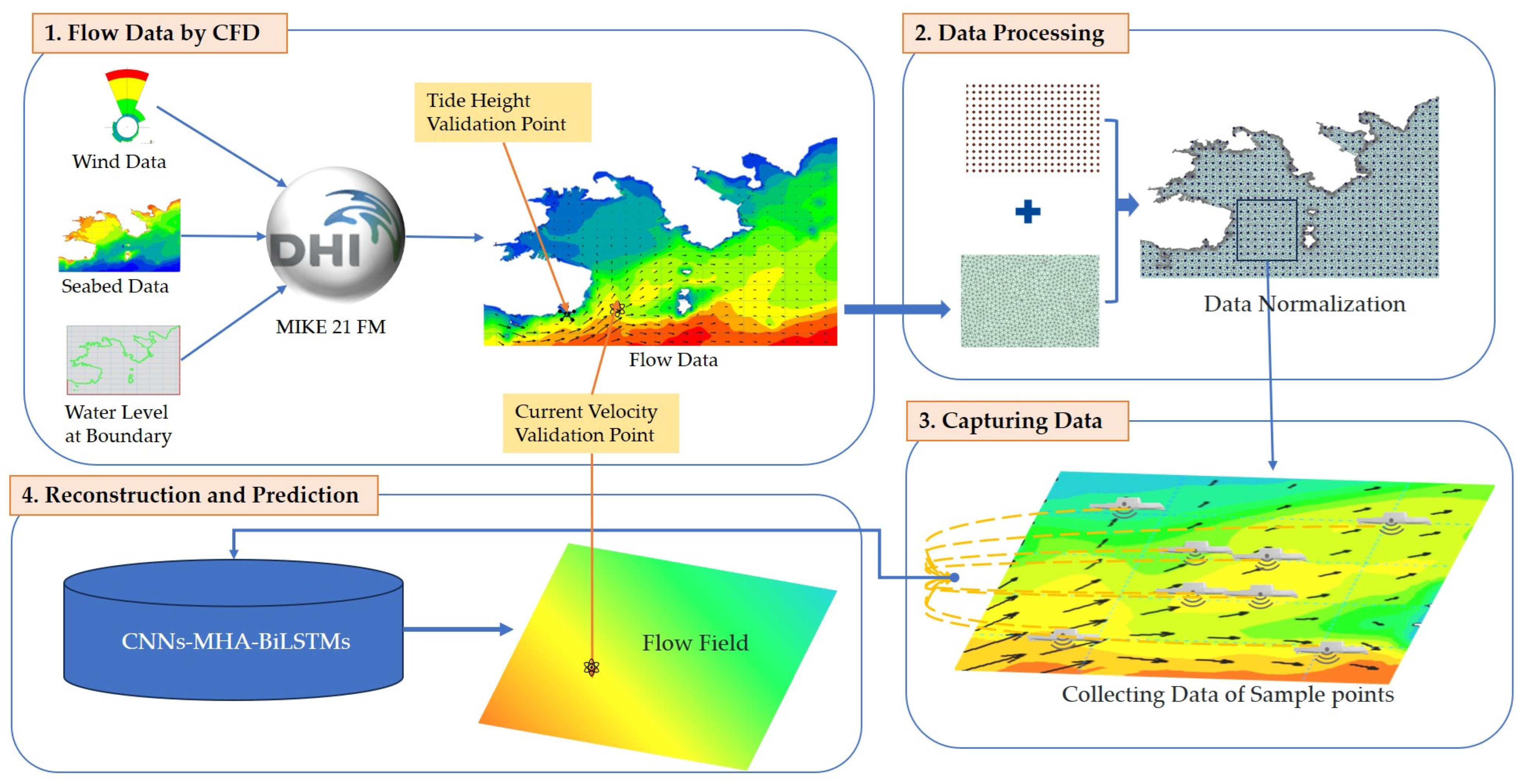
First, the MIKE21 flow model (FM) commercial coast and marine modelling software, released 2014, were used to solve the entire flow field, thereby generating a comprehensive database by solving the hydrodynamic equations on a two-dimensional unstructured mesh. The database provided reliable data for subsequent analysis and modelling by capturing information over the entire area.

Second, the numerical solutions corresponding to the measured points were extracted from the database and compared with the measured values to verify the accuracy and reliability of the numerical solutions.

Third, the original unstructured mesh data were transformed into regular data by sampling the data at fixed intervals (e.g., 0.01°) within the selected area.

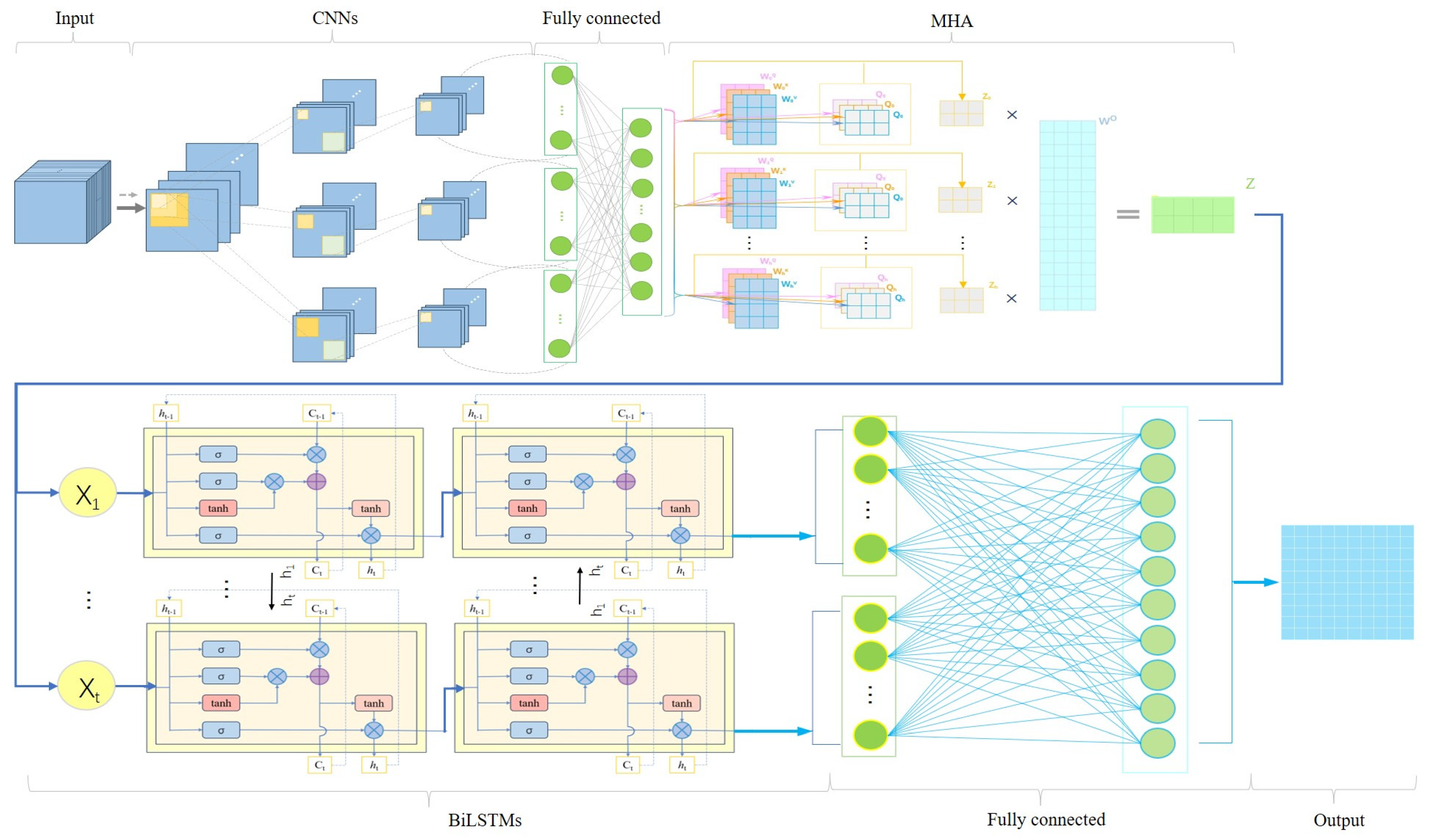
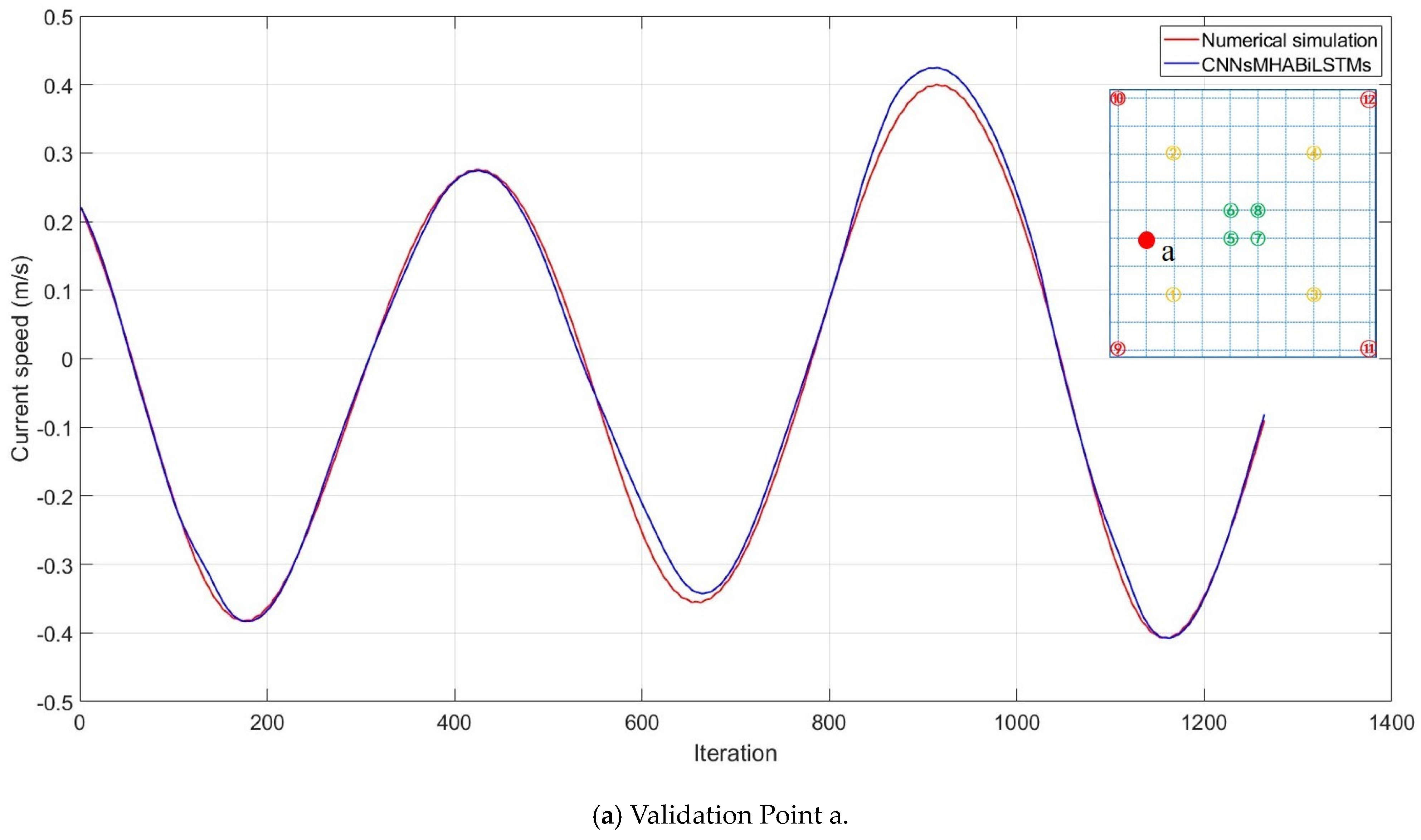
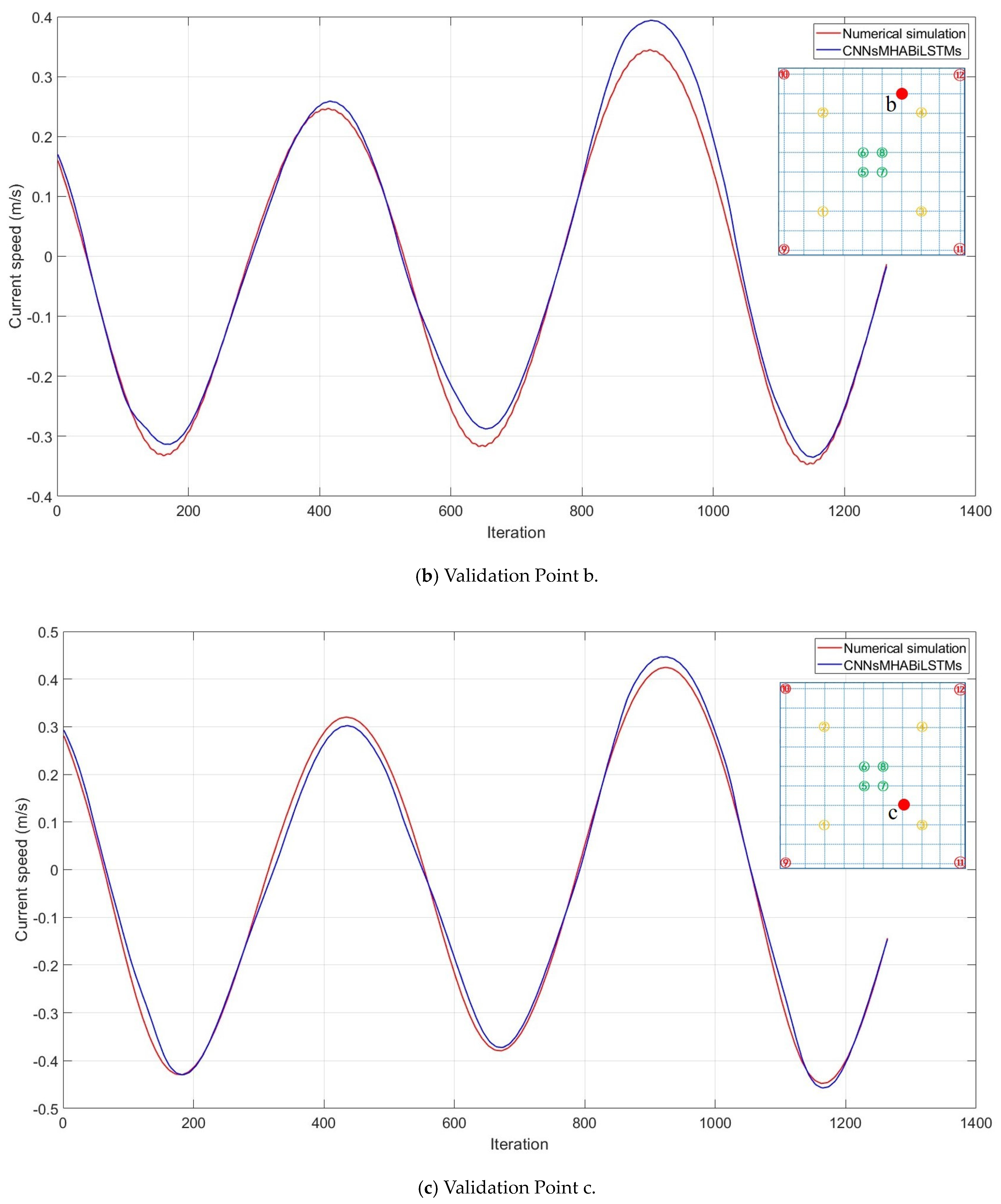
Fourth, the CNNs–MHA–BiLSTMs model was employed to predict the velocities of points in the flow based on the input data, including wind velocity components, tide height, and previous flow velocities, in order to forecast them.

Finally, the application of the CNNs–MHA–BiLSTMs model combined with the flow velocities in the current moment for these points as the inputs enabled the prediction of flow velocities over an extended surface or a larger area in the next moment. The purpose of this step is to structure the points into surface data by leveraging the spatiotemporal prediction capability of the model.

3.1. Development of the Flow Field Database

In our study, one of the significant challenges we face is the scarcity of measured data. Such data are crucial for training and validating AI models aimed at predicting complex fluid environments. Given the time-consuming and costly nature of field measurements, CFD methods become an invaluable tool for obtaining alternative data; CFD simulations can mimic fluid motion under various conditions, generating detailed and diverse time-series flow field data.

To ensure that CFD-generated data closely resemble real-world data, we implemented a series of precise settings during simulations. Although CFD data may not perfectly match real-world fluid fields, it provides a valuable training foundation, especially in the absence of direct observation data. This approach based on CFD simulation data aids in progressively achieving more precise prediction and higher efficiency in engineering applications and lays a foundation for adopting precise measurement data to replace simulated data for algorithm training in the future.

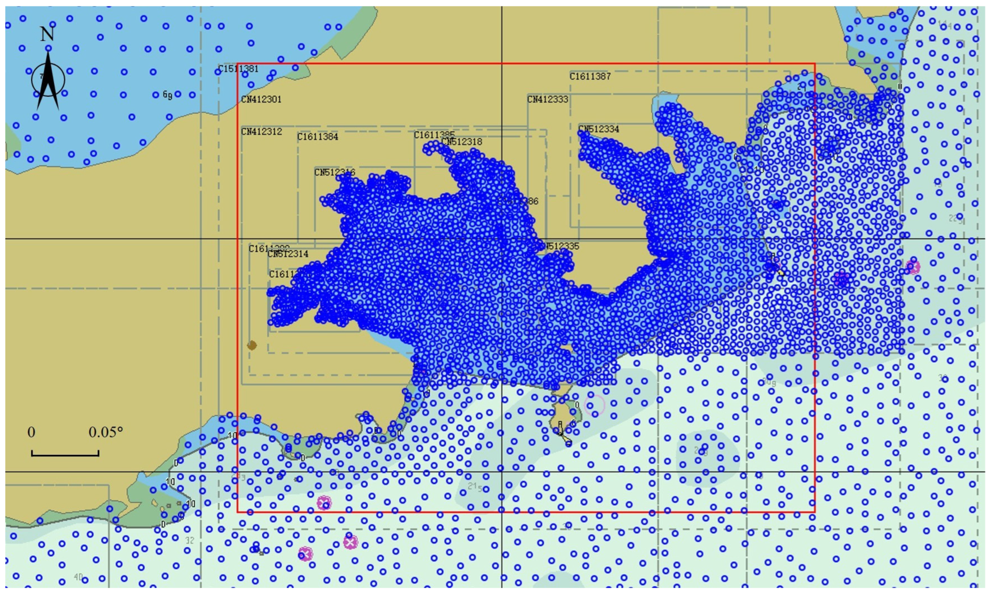
The MIKE21 FM software, which is based on the finite volume method using unstructured meshes, takes the ocean areas around Dalian Port, China, as a case study for numerical simulations. The objective was to obtain data for the entire two-dimensional ocean surface domain and subsequently validate the data. The topographic and bathymetric data used for the simulation area were obtained from CN412301, CN412312, and CN412333 electronic nautical charts. The computational field is delineated by the red square in Figure 3, with the blue marks indicating the locations of the depth sampling points, as listed in

Table 1. Coordinates of the vertices of the simulation area in Dalian.

Point	Latitude	Longitude
A	38°49′02.05″ N	121°34′50.52″ E
B	38°49′02.05″ N	122°01′08.48″ E
C	39°05′00.57″ N	122°01′08.48″ E
D	39°05′00.57″ N	121°34′50.52″ E

.

Grid independence, a pivotal aspect of numerical simulations, ensures that results remain consistent and convergent as the computational grid is refined. Employing various element resolutions (

Table 2. The counts of elements and nodes for each case.

Case	Nodes	Elements
I	45,437	82,660
II	24,207	40,691
III	13,580	22,047

) verifies how numerical solutions accurately reflect physical phenomena, free from grid-related artefacts, thereby enhancing the reliability and validity of our findings. In this study, rigorous grid independence tests were conducted to validate our result.

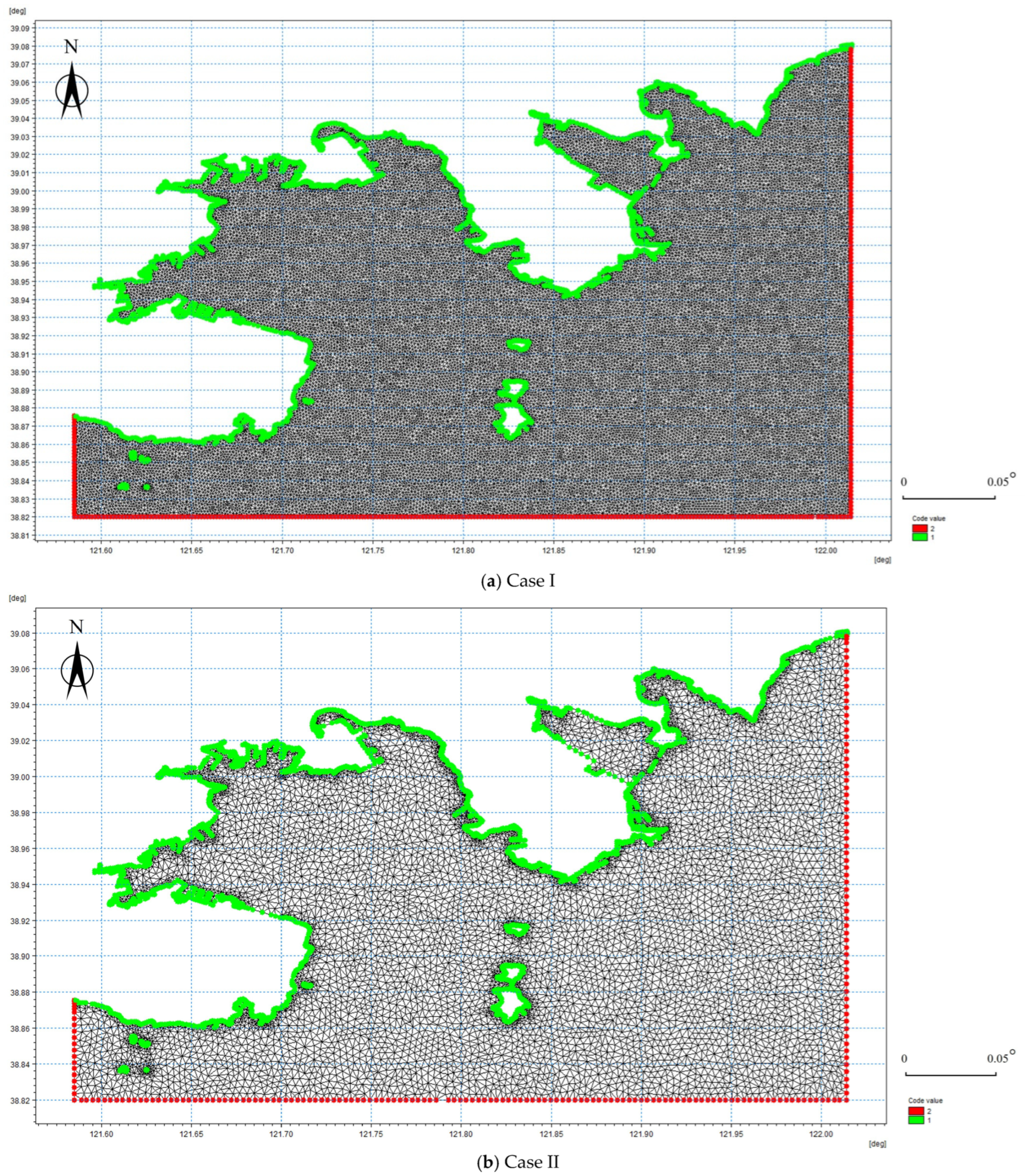
These meshes of different cases are shown as (a), (b), and (c) in Figure 4, where the green data markers denote the land boundaries and the red data markers denote the open boundaries. The selection of triangular meshes was a result of the complex coastline of our study area, where triangular meshes perform better than rectangular meshes in dealing with intricate shoreline structures. Triangular meshes can flexibly adapt to irregular boundaries, automatically adjusting the positions of mesh nodes to fit the curves and protrusions of complex coastlines and capture small geographical features to achieve higher precision.

Ocean currents are driven by various forces, and the wind pressure on the ocean surface is one of the key factors. The input parameter for this study was the wind velocity at a height of 10 m above the ocean surface, which was used to compute the average wind velocity over the area [22]. Meteorological data were obtained from the Xihe Energy Big Data Platform [23].

The temperature and salt level were set by a positive pressure equation; Manning’s M was 30 m^1/3/s, the time step was calculated to be 30s, and the CFL number was set to 0.8 to avoid model divergence. The influence of Coriolis force and tidal potential was not considered since the simulation area was small. Wave radiation stress was considered negligible because its influence was overshadowed by the stronger and more consistent forces created by tidal movements [24,25]. For more detailed parameter settings, refer to [26]. Closed boundaries were assigned to coastal areas, whereas open boundaries with Flather boundary conditions were applied to open areas outside the coast. The water level at the open boundaries was set as the tidal water level, which varied with time. The water depth data were obtained by sampling depth points marked on electronic nautical charts and interpolating them to achieve a more continuous and accurate distribution of the water depth. 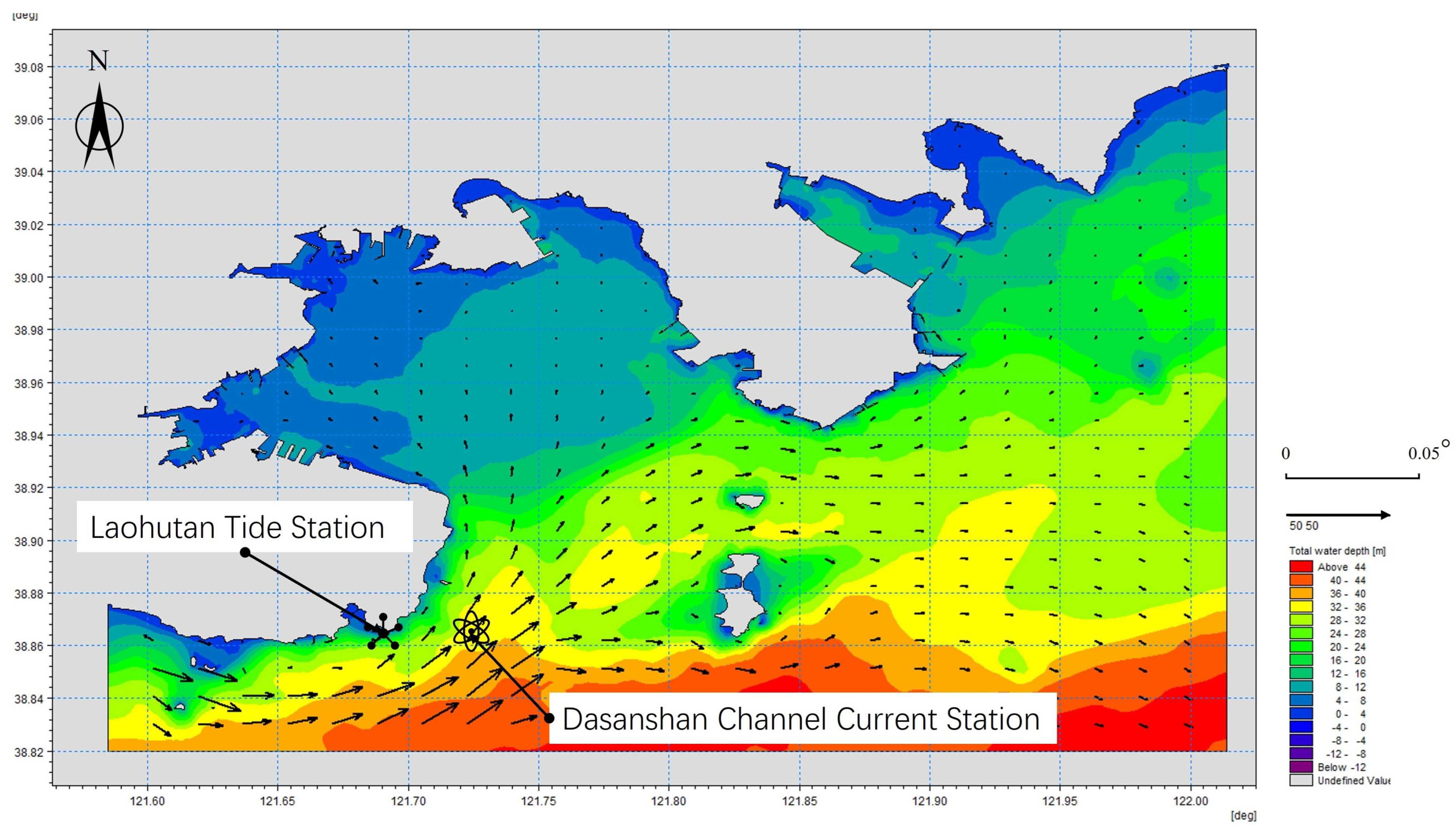Figure 5 illustrates both the water depth distribution and flow velocity vectors at a scale magnified 50 times.

To verify and validate the accuracy of the MIKE21 FM numerical model, validation was performed during spring tides. The numerical simulations were conducted from 8th January 2024 (08:00) to 22nd January 2024 (08:00), with the results outputted every 30 s. The simulation period for the spring tides was selected from 15th January 2024 (08:00) to 16th January 2024 (08:00). The results were compared with the observed tide height data from the Laohutan tide station in Dalian city and the observed current speed and direction data from the Dasanshan Channel current station in Dalian city, provided by the National Ocean Data and Information Service, which is a government-funded public institution under the State Oceanic Administration of China [27]. The station coordinates are presented in

Table 3. Coordinates of the tide and current stations in Dalian.

Station Name	Station Type	Latitude	Longitude
Laohutan	Tide station	38°52′00.12″ N	121°40′59.88″ E
Dasanshan Channel	Current station	38°52′00.12″ N	121°43′59.88″ E

.

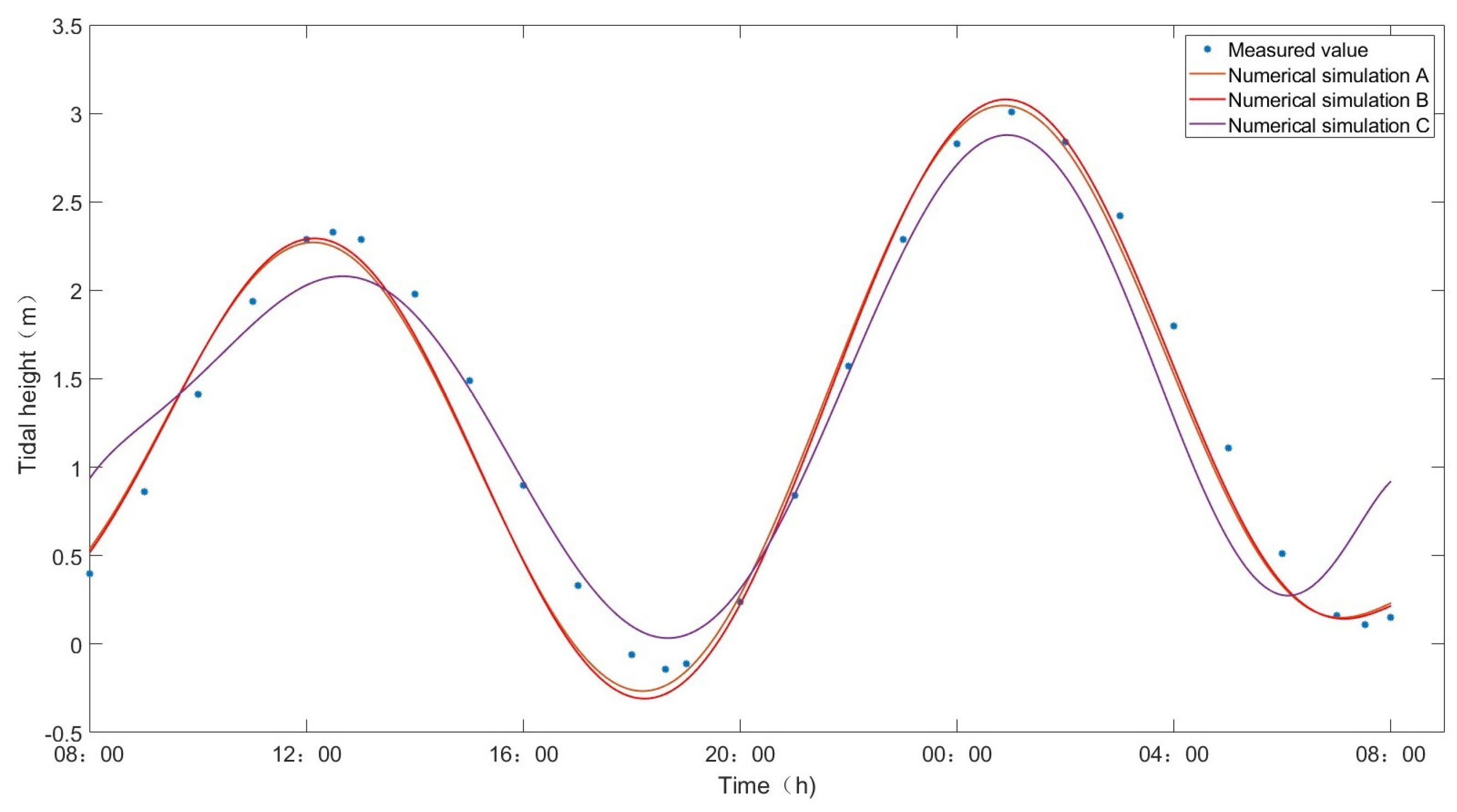
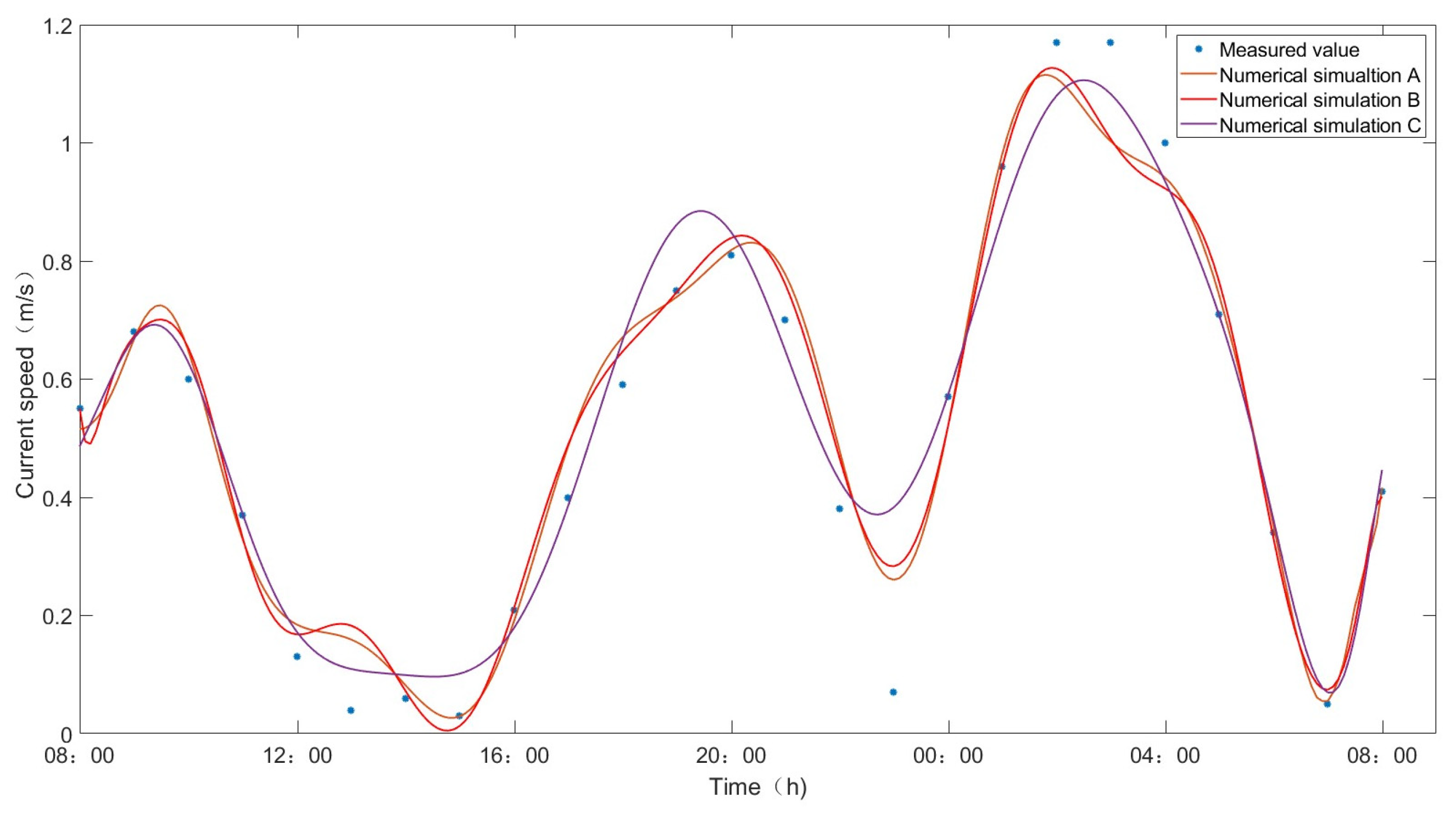
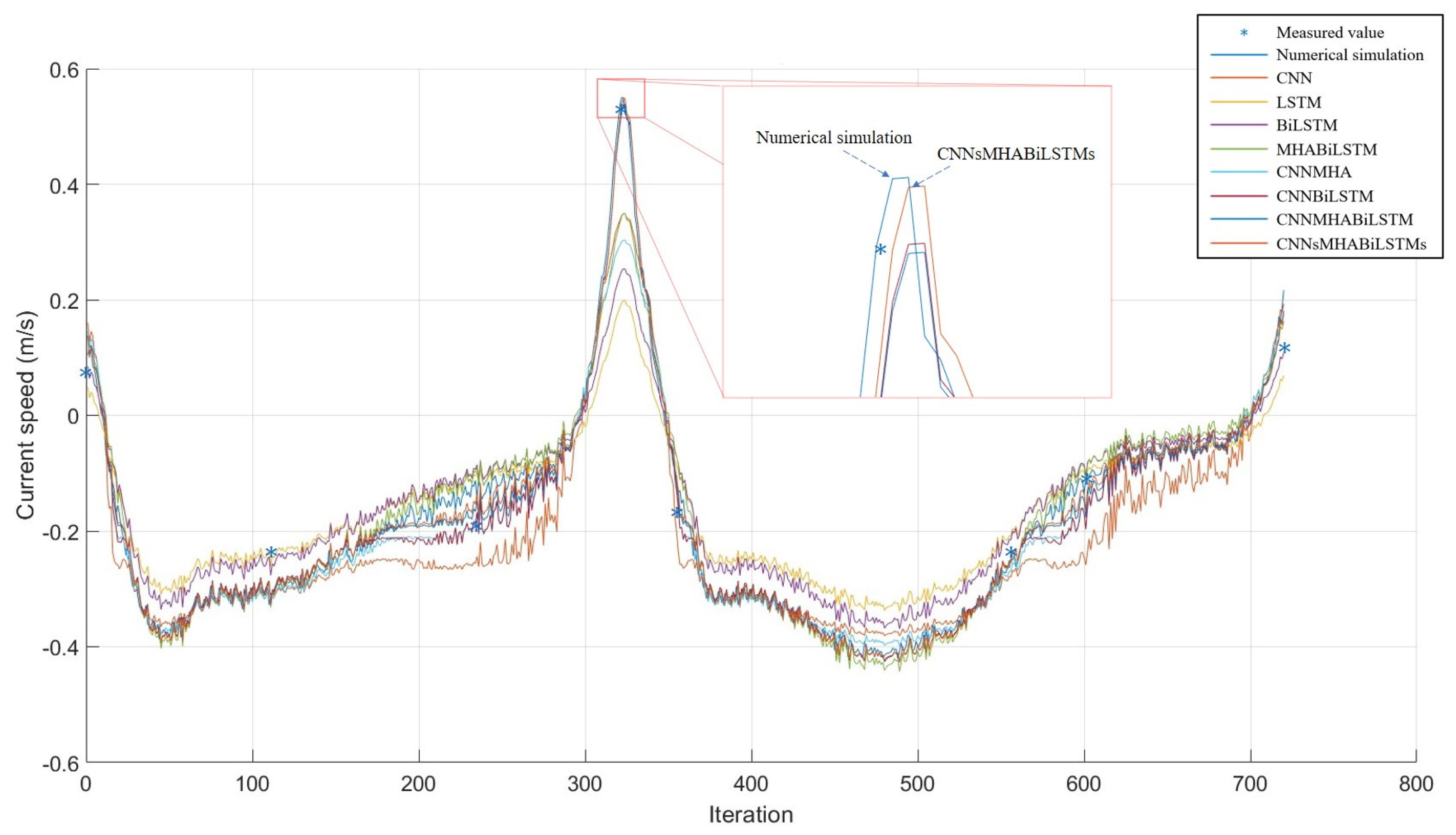
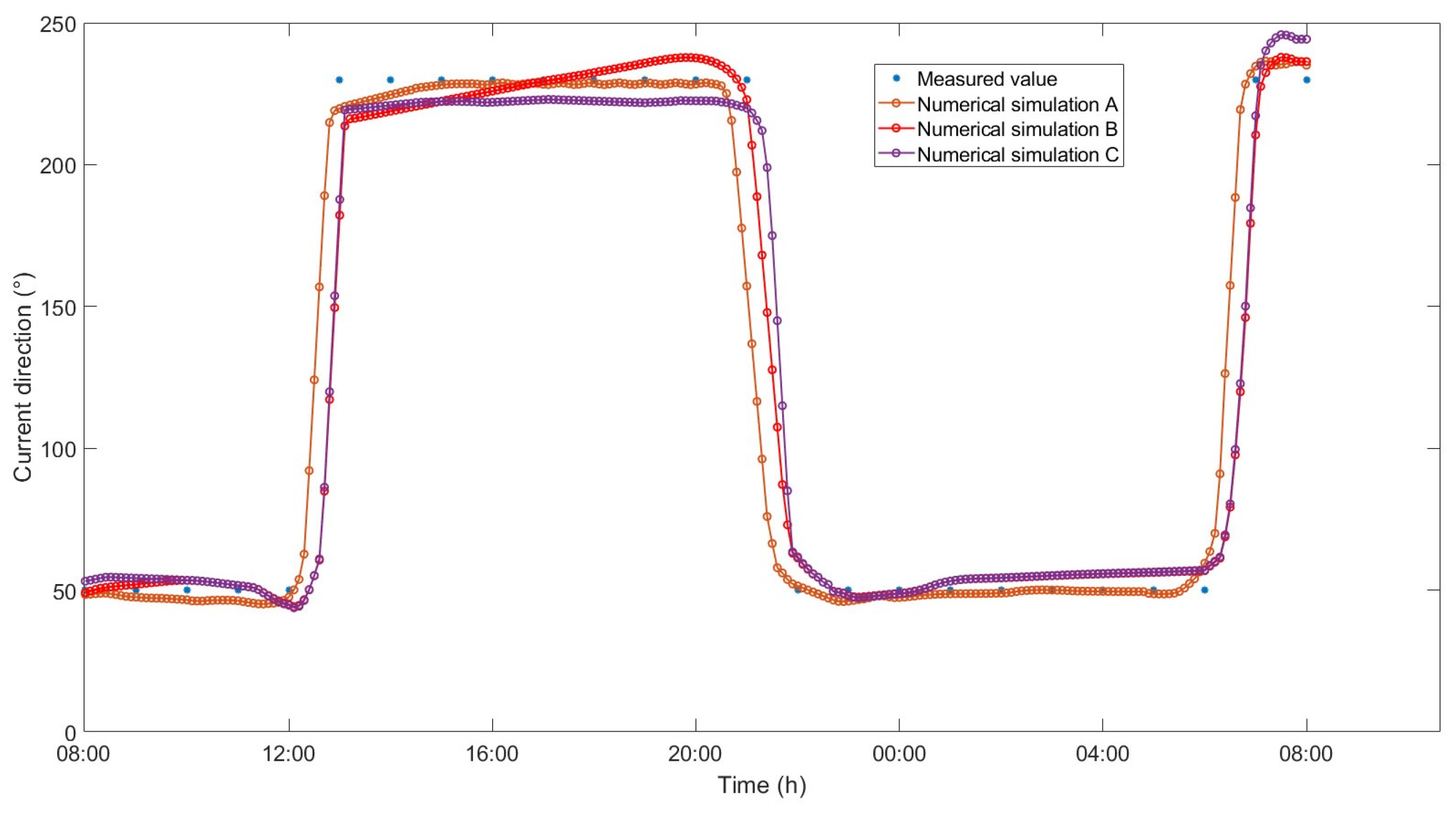
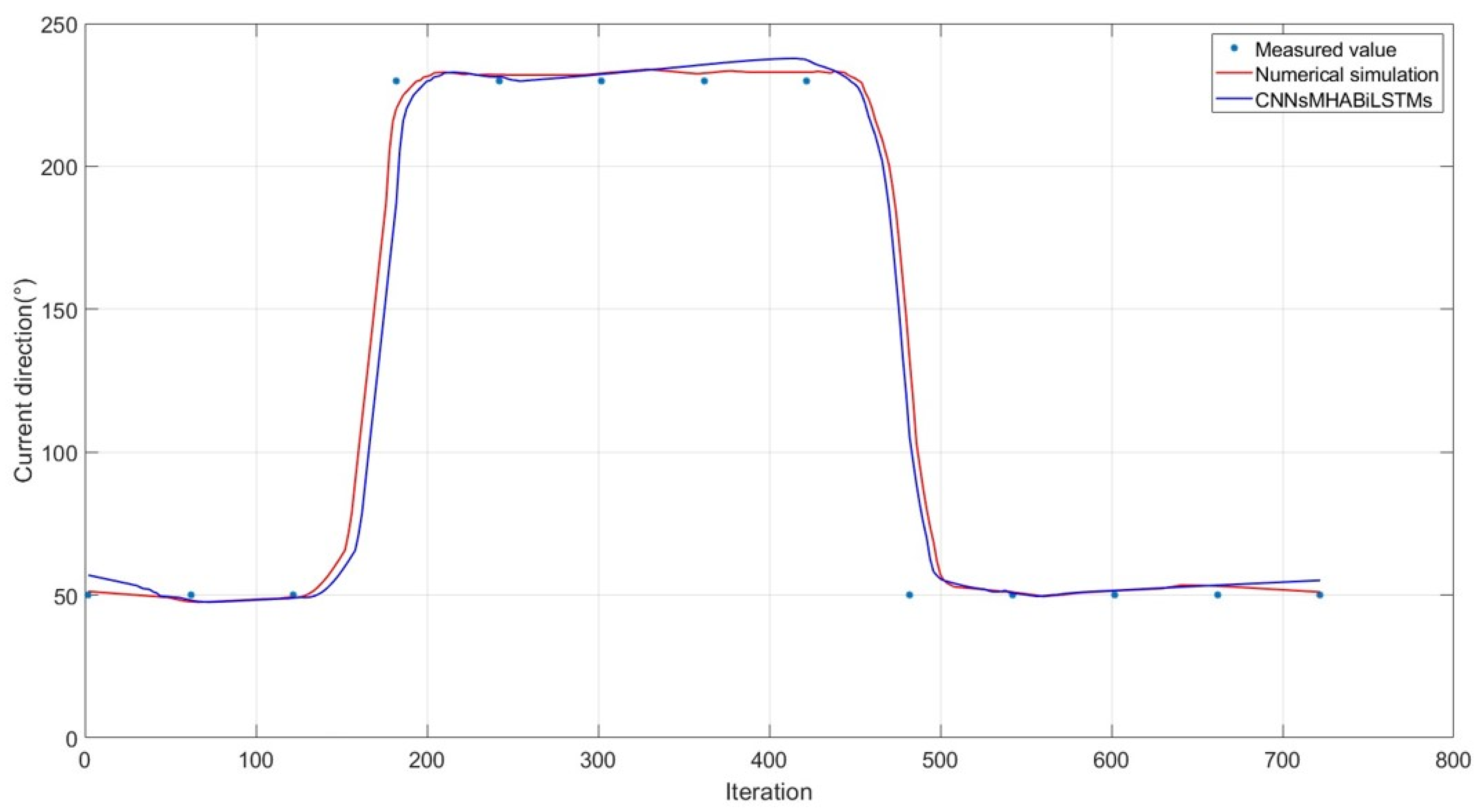
The tide height validation results for Laohutan are shown in Figure 6. The current speed validation results for the Dasanshan Channel are shown in Figure 7, whereas the current direction validation results for the Dasanshan Channel are shown in Figure 8.

In this study, three metrics were used to evaluate the performance of the MIKE21 FM, namely, the mean absolute percentage error (MAPE), root mean squared error (RMSE), and coefficient of determination (R²). These metrics place different emphasis on the prediction results of deep learning models. The RMSE, MAPE, and R² were calculated using Equation (11), Equation (12), and Equation (13), respectively.

$$RMSE=\sqrt{{\displaystyle \frac{1}{n}}{\sum }_{i=1}^n{\left|{\widehat{y}}_i-{\overline{y}}_i\right|}^2}$$

(11)

$$MAPE={\displaystyle \frac{100\%}{N}}{\displaystyle {\sum }_{i=1}^N}\left|{\displaystyle \frac{{\widehat{y}}_i-y_i}{y_i}}\right|$$

(12)

$$R^2=1-{\displaystyle \frac{{\sum }_{i=1}^N{({\widehat{y}}_i-y_i)}^2}{{\sum }_{i=1}^N{\left({\overline{y}}_i-y_i\right)}^2}}$$

(13)

In these equations, N is the maximum number of iterations, $y_i$ is the actual value, ${\widehat{y}}_i$ is the predicted value, and ${\overline{y}}_i$ is the mean of the actual values. According to the validation results for the tide height, current velocity, and current direction, the numerical simulation results at the monitoring sites were generally consistent with the measured values. The evaluation metrics of the MIKE21 FM of various element resolutions used to predict the single-point flow field characteristics are presented in

Table 4. Evaluation metrics of the MIKE21 FM of various elements resolution.

Item	Case	RMSE	MAPE (%)	R2
Tide height	I	0.2103 m	9.64	0.9858
	II	0.2332 m	10.12	0.9791
	III	0.3387 m	16.94	0.9577
Current speed	I	0.0623 m/s	15.60	0.9564
	II	0.0685 m/s	15.97	0.9529
	III	0.0942 m/s	21.18	0.9022
Current direction	I	8.7096°	4.70	0.9845
	II	11.7174°	7.03	0.9811
	III	13.3674°	7.52	0.9717

.

Through the analysis of three numerical simulations (Case I, II, and III) using error metrics such as RMSE, MAPE, and R², several important conclusions regarding grid independence can be drawn. First, Case I demonstrates the best performance in capturing THE water level, flow speed, and flow direction, exhibiting remarkable stability and high accuracy, indicating that the simulation results are relatively insensitive to grid variations at the defined resolution. In contrast, Case II, while showing slightly reduced performance, still maintains a high level of accuracy, suggesting that a moderate reduction in the number of nodes and elements does not significantly impact THE results. Conversely, Case III presents a contrasting scenario, with marked increases in RMSE and MAPE, as well as a decline in R², indicating a strong grid dependence. This is particularly evident with only 13,580 nodes and 22,047 elements, leading to a substantial reduction in the accuracy of the simulation results. This indicates that an overly coarse grid can lead to the loss of critical details, resulting in larger errors. Considering the overall computational power, the analysis of the three cases must balance grid refinement with the efficient use of computational resources. Case I excels in accuracy and stability; however, its high number of nodes and elements (45,437 nodes and 82,660 elements) implies greater computational resource and time consumption, which might lead to inefficiency or resource exhaustion. Case II maintains high precision while slightly reducing the number of nodes and elements, indicating that a reasonable grid resolution can achieve a balance between accuracy and computational power consumption, resulting in a satisfactory outcome. Based on these results, it can be deduced that the MIKE21 FM can accurately predict the flow field characteristics within the area of interest.

3.2. Supplementary Validation

Due to the scarcity of publicly available data points on currents, velocity, and tide height in the waters near Dalian, to ensure the reliability of the CFD data, we conducted detailed numerical simulations for another coastal area (Lianyungang). Lianyungang is located in the central region of China’s coastline, adjacent to the Yellow Sea. These simulations were rigorously validated using tidal and current station data that are publicly available for that region. By meticulously comparing the model outputs with actual field measurement data, we achieved a high level of consistency, significantly enhancing the accuracy and reliability of the initial data input for the AI model.

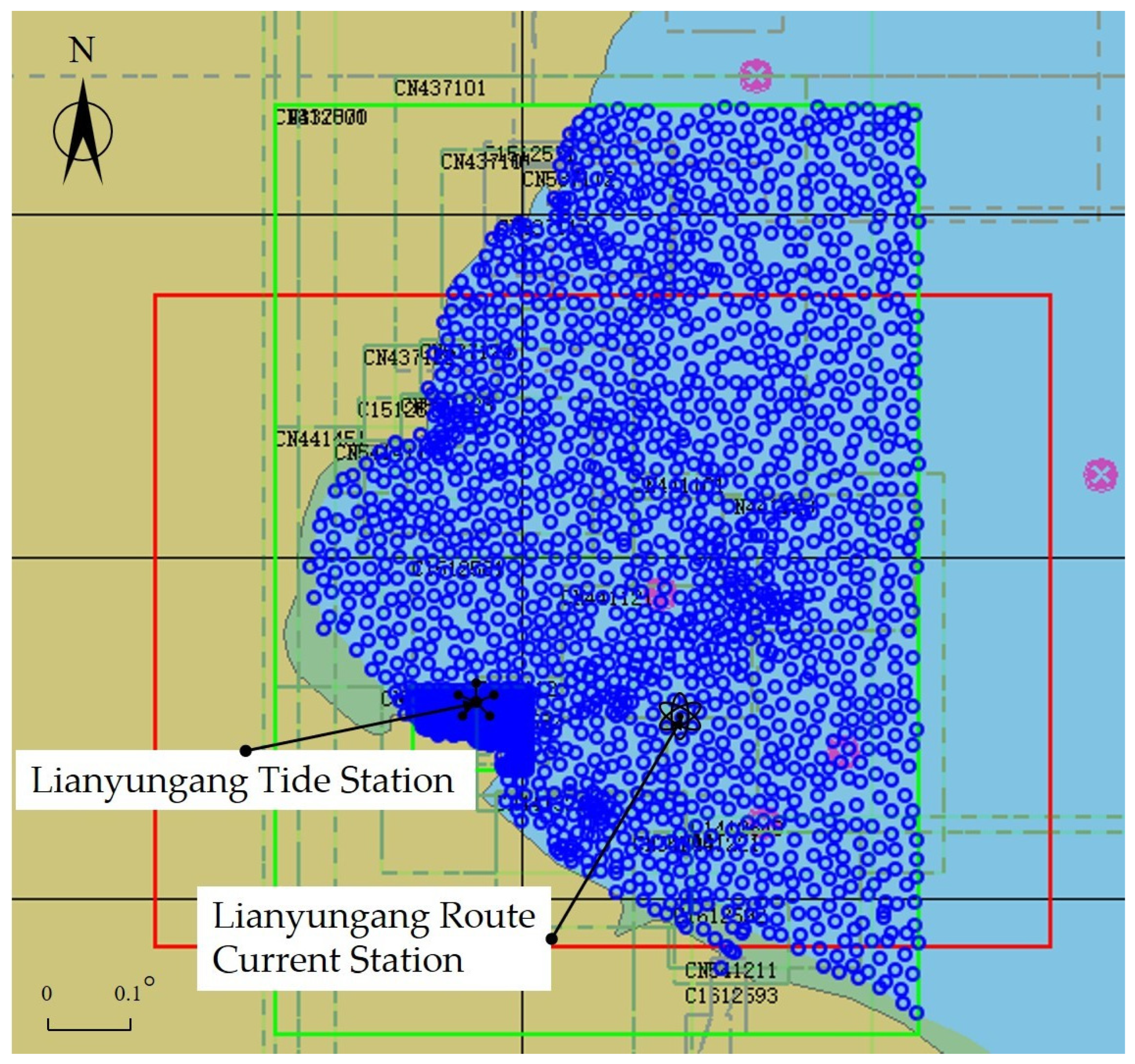
The topographic and bathymetric data used for the simulation area were obtained from CN337001 and CN541112 electronic nautical charts. The computational field is delineated by the green square in Figure 9, with the blue marks indicating the locations of the depth-sampling points.

A two-dimensional unstructured grid was used for discretization, consisting of 36,067 computational nodes and 67,125 triangular elements within the computational domain, as shown in Figure 10. The green markers denote the land boundaries, while the red markers indicate the open boundaries.

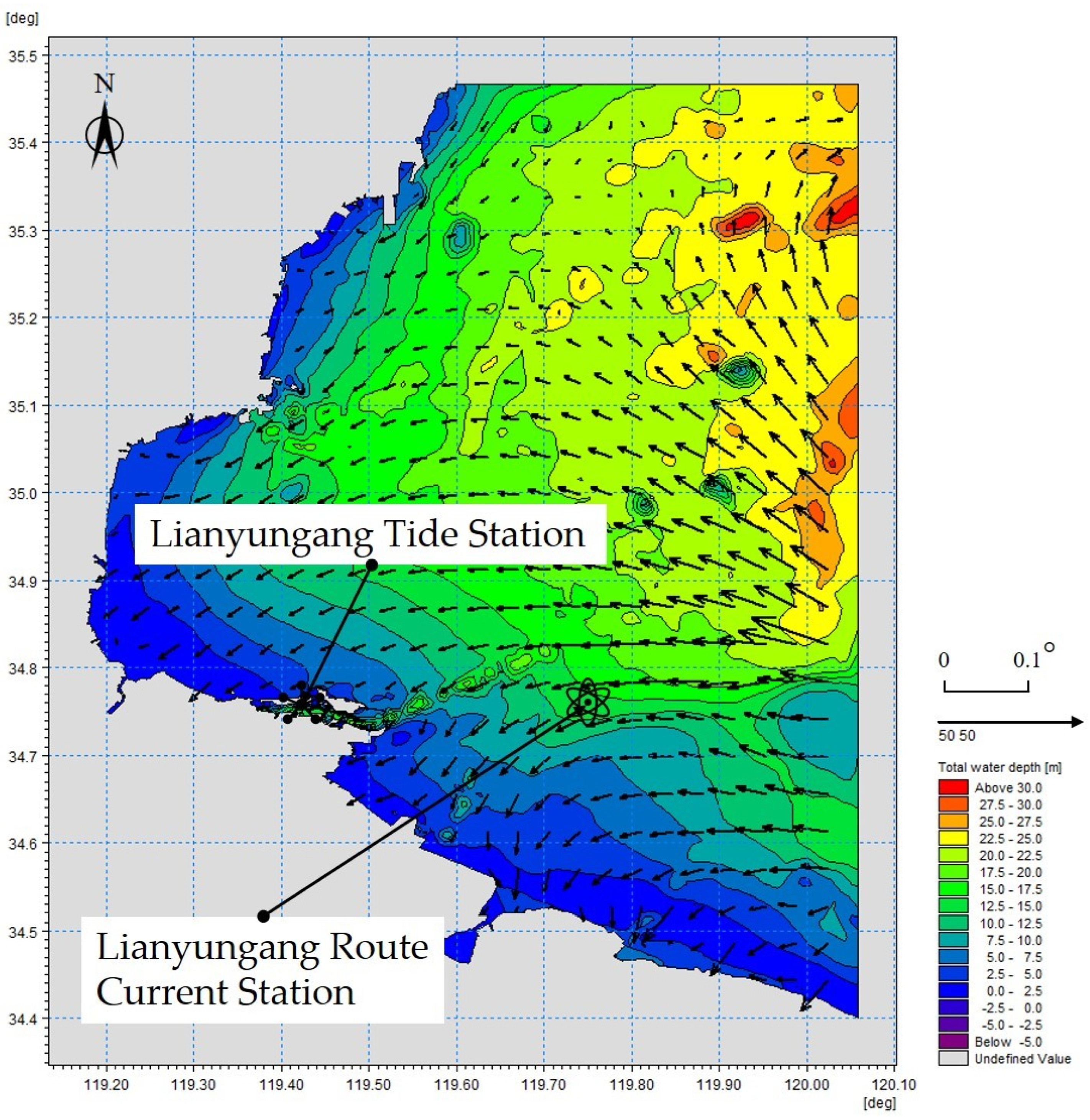
The meteorological data are also sourced from the Xihe Energy Big Data Platform. Aside from changing Manning’s M to 28 m^1/3/s, this approach and other parameters remain the same as those used in the previous CFD model setup for the waters near Dalian. Figure 11 illustrates both the water depth distribution and flow velocity vectors, magnified 50 times.

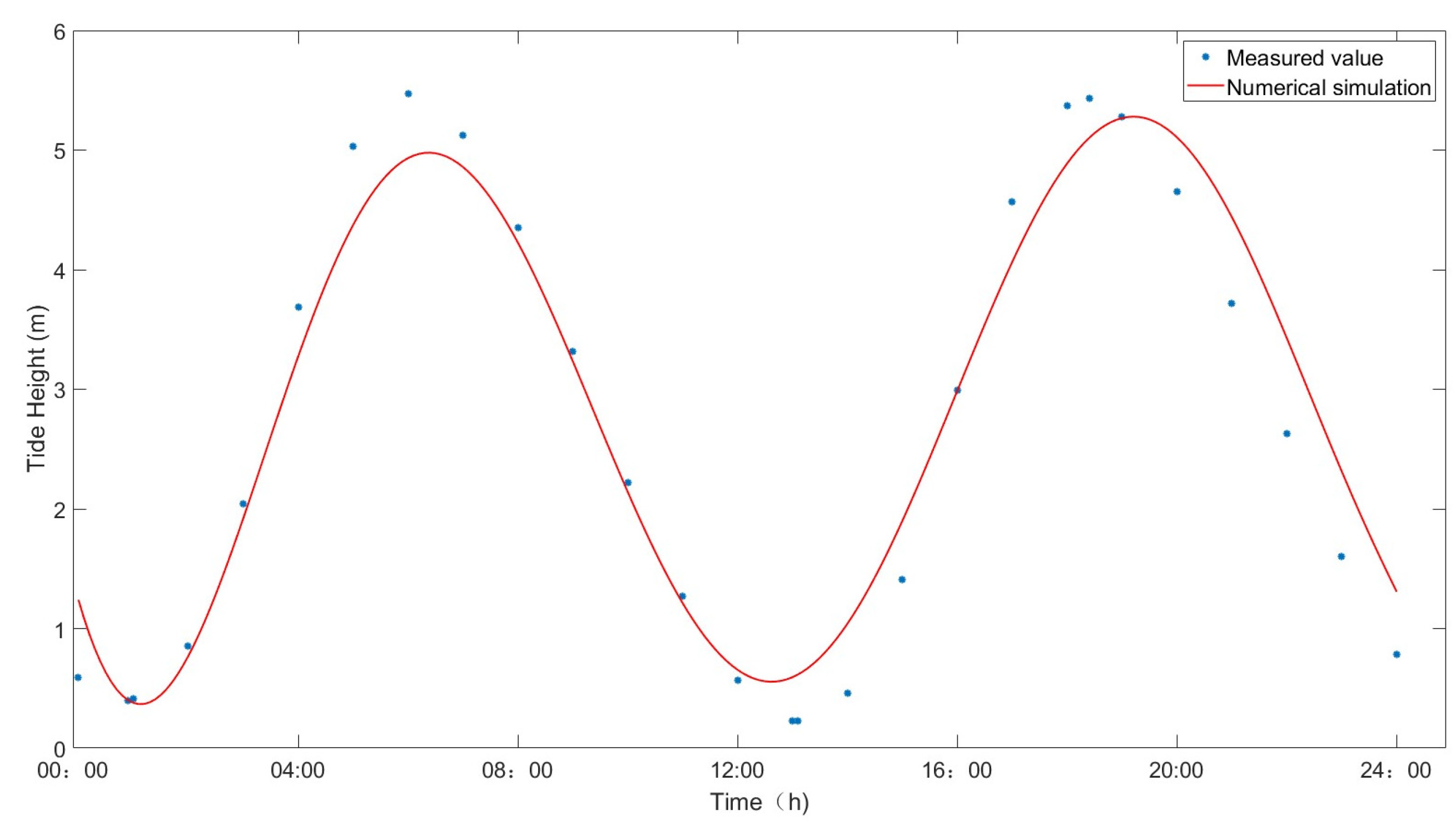
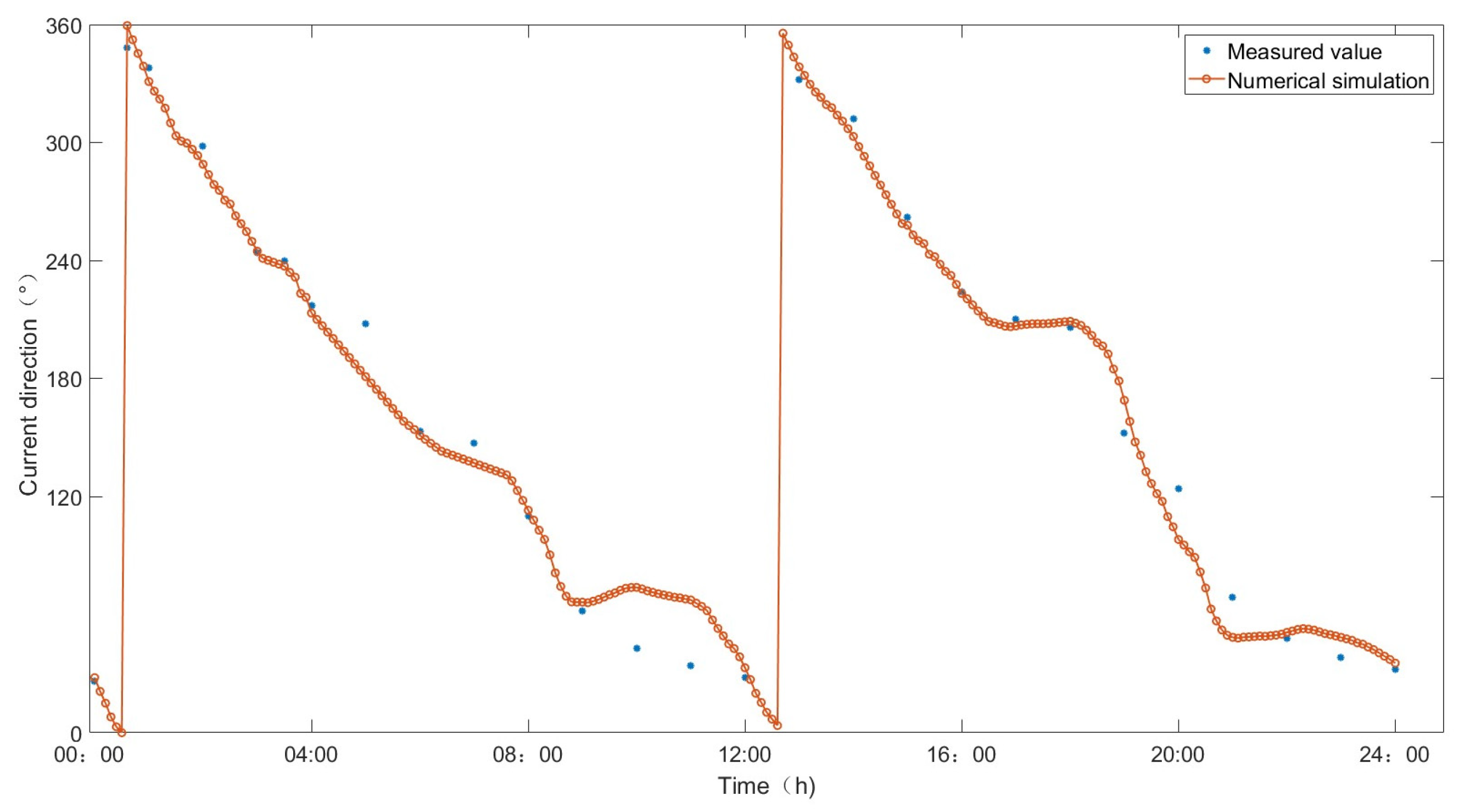
To verify and validate the accuracy of the MIKE21 FM, results were outputted every 30 s. The simulation period for the spring tides was chosen from 9 April 2024 (00:00) to 10 April 2024 (00:00). The results were then compared with the observed tide height data from the Lianyungang tide station and the observed current speed and direction data from the Lianyungang Route current station, both located in Lianyungang city. These data were provided by the National Ocean Data and Information Service, which is a government-funded public institution under the State Oceanic Administration of China [27]. The station coordinates are listed in

Table 5. Coordinates of the tide and current stations.

Station Name	Station Type	Latitude	Longitude
Lianyungang	Tide station	34°45′00.00″ N	119°25′00.12″ E
Lianyungang Route	Current station	34°45′00.00″ N	119°45′00.00″ E

.

The verification result of tide height is presented in Figure 12, while the verification results of current speed and direction are displayed in Figure 13 and Figure 14, respectively.

The evaluation indicators for CFD simulations are shown in

Table 6. Evaluation metrics of the MIKE21 FM in Lianyungang.

Item	RMSE	MAPE (%)	R2
Tide height	0.2423 m	16.62	0.9510
Current speed	0.0979 m/s	13.92	0.9612
Current direction	15.9101°	6.52	0.9795

.

The approach taken to conduct CFD simulations and validations in the sea area adjacent to Lianyungang, through the selection of an additional computational domain for verification purposes, addressed the limitation of having a restricted number of validation points within our initial domain. The finding that the data accuracy across multiple domains at validation points is comparatively high further underscores the dependability and trustworthiness of the CFD data referenced in our earlier content.

3.3. Data Processing

The use of a two-dimensional unstructured mesh for horizontal space discretization of the MIKE21 FM can lead to nonuniform element sizes, irregular node arrangements, and varying inter-node distances, posing a challenge for deep learning models that aim to extract spatial features. To address these issues effectively, a sparse regularization data-processing method was adopted.

Initially, transforming original unstructured mesh data into a regularly spaced format with a point spacing of 0.01° yielded a sparser representation; this transformation enabled our deep learning model to better capture the spatial characteristics of current variations. Subsequently, we reduced the number of computational nodes from 24,207 to just 593, limiting each cell data point to one and extending the time intervals from 30 s to 120 s. This not only diminished the volume of the dataset but also standardized the data format, thereby enhancing regularity and optimizing subsequent analytical and modelling processes.

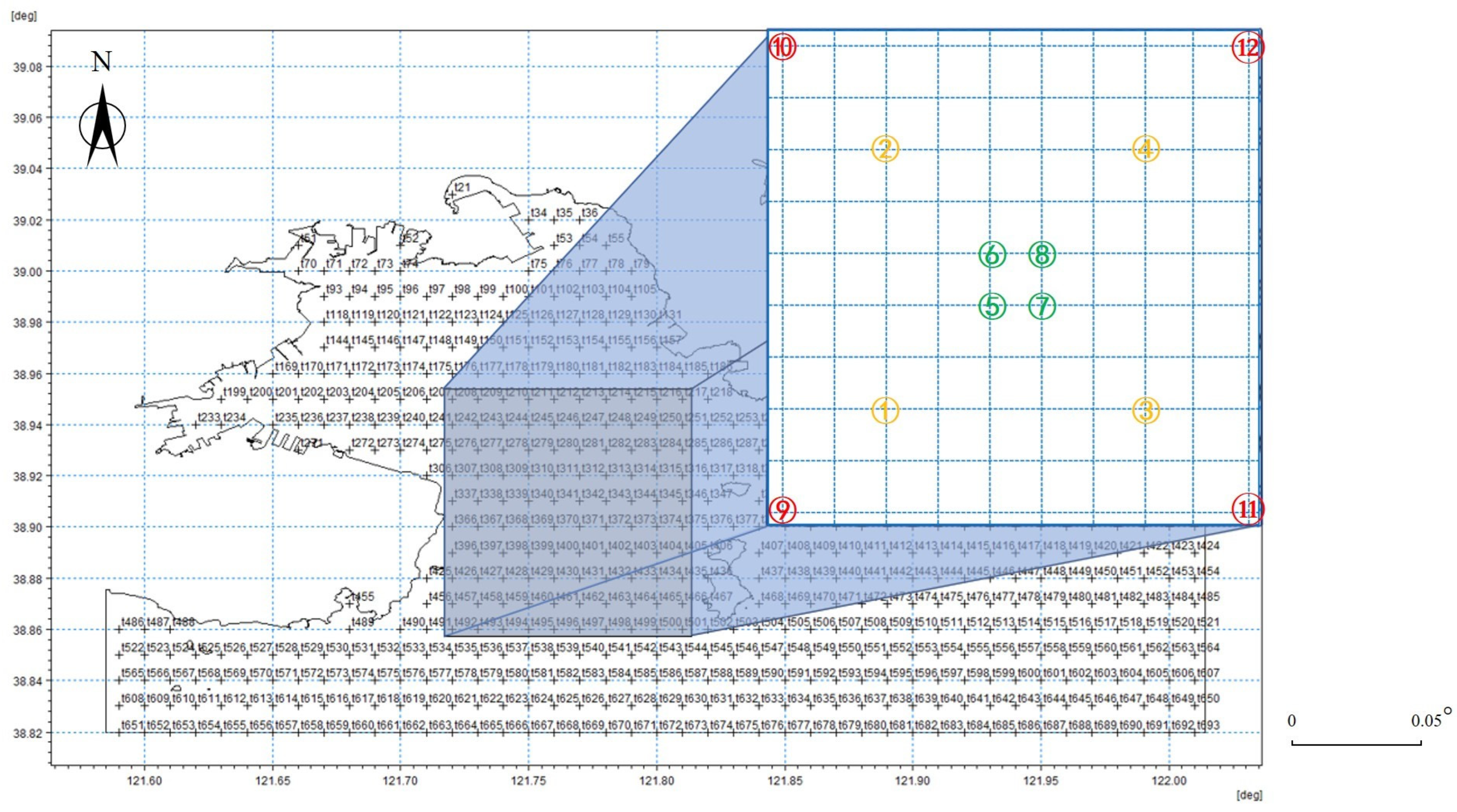
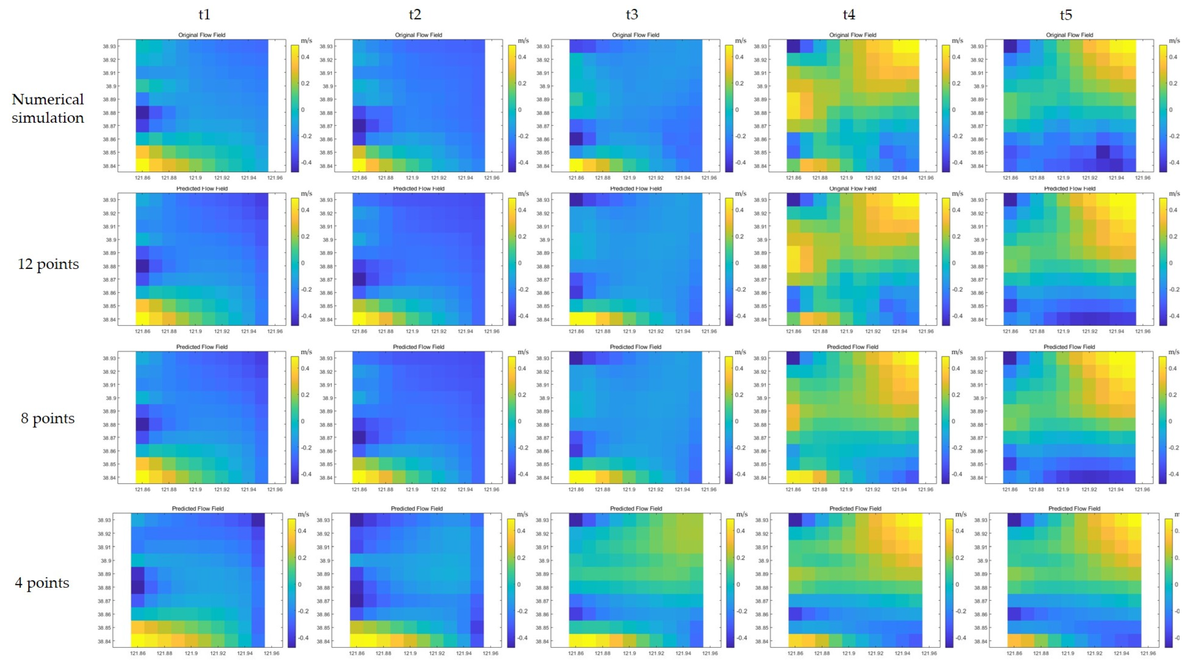
Following this transformation process, a specific area measuring 10 km × 10 km was selected for subsequent model training and testing purposes, as shown in Figure 15. Here, the first experiment was sampled by four points (as indicated by the green circles), the second experiment was sampled by eight points (as indicated by the green and yellow circles), and the third experiment was sampled by 12 points (as indicated by the green, yellow, and red circles), providing the flow field characteristics across quadrants, including velocity variations along the diagonals. This study enhanced the adaptability and robustness through the addition of white noise variance (0.0001), which aligned with complex real-environment interferences.

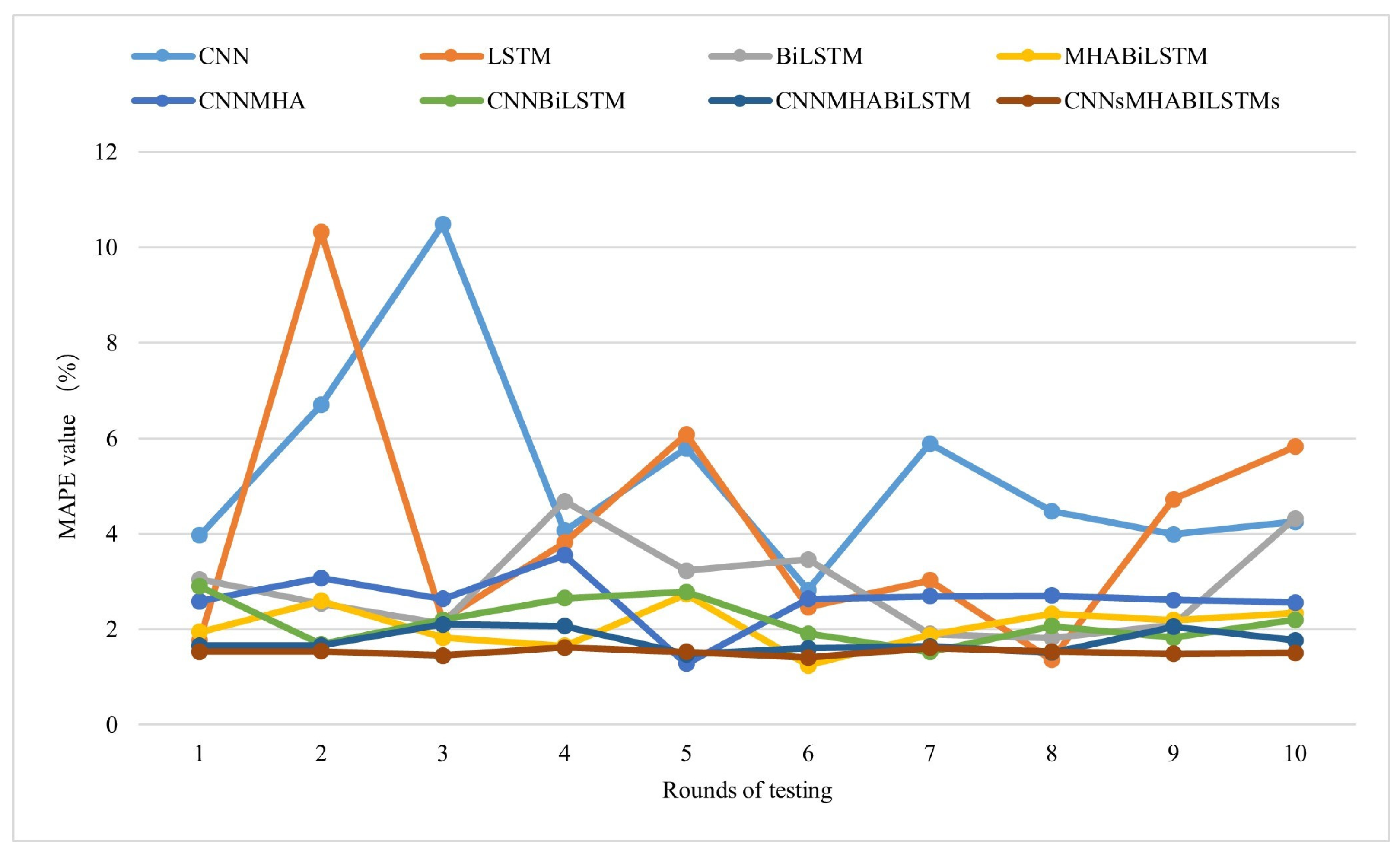
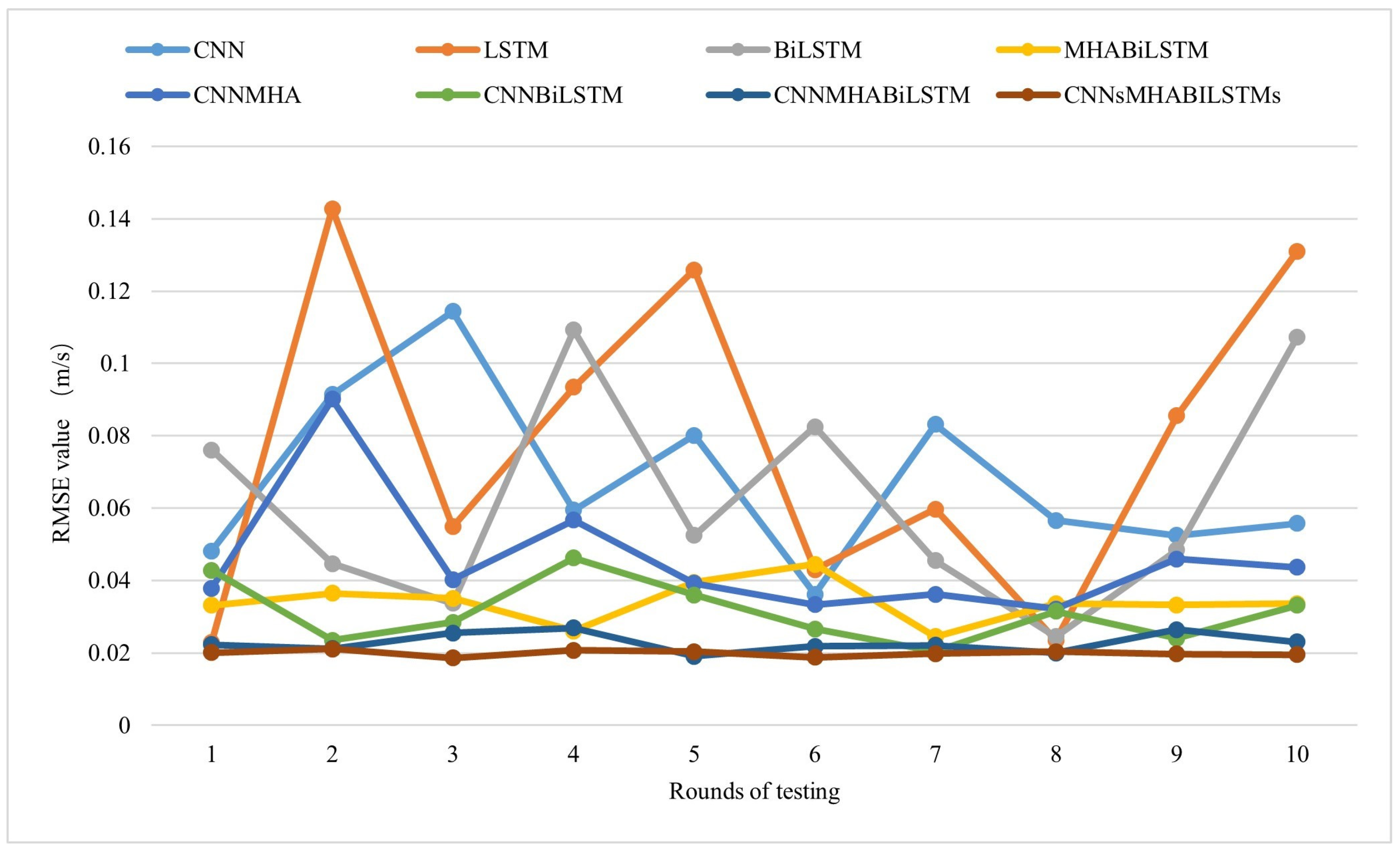
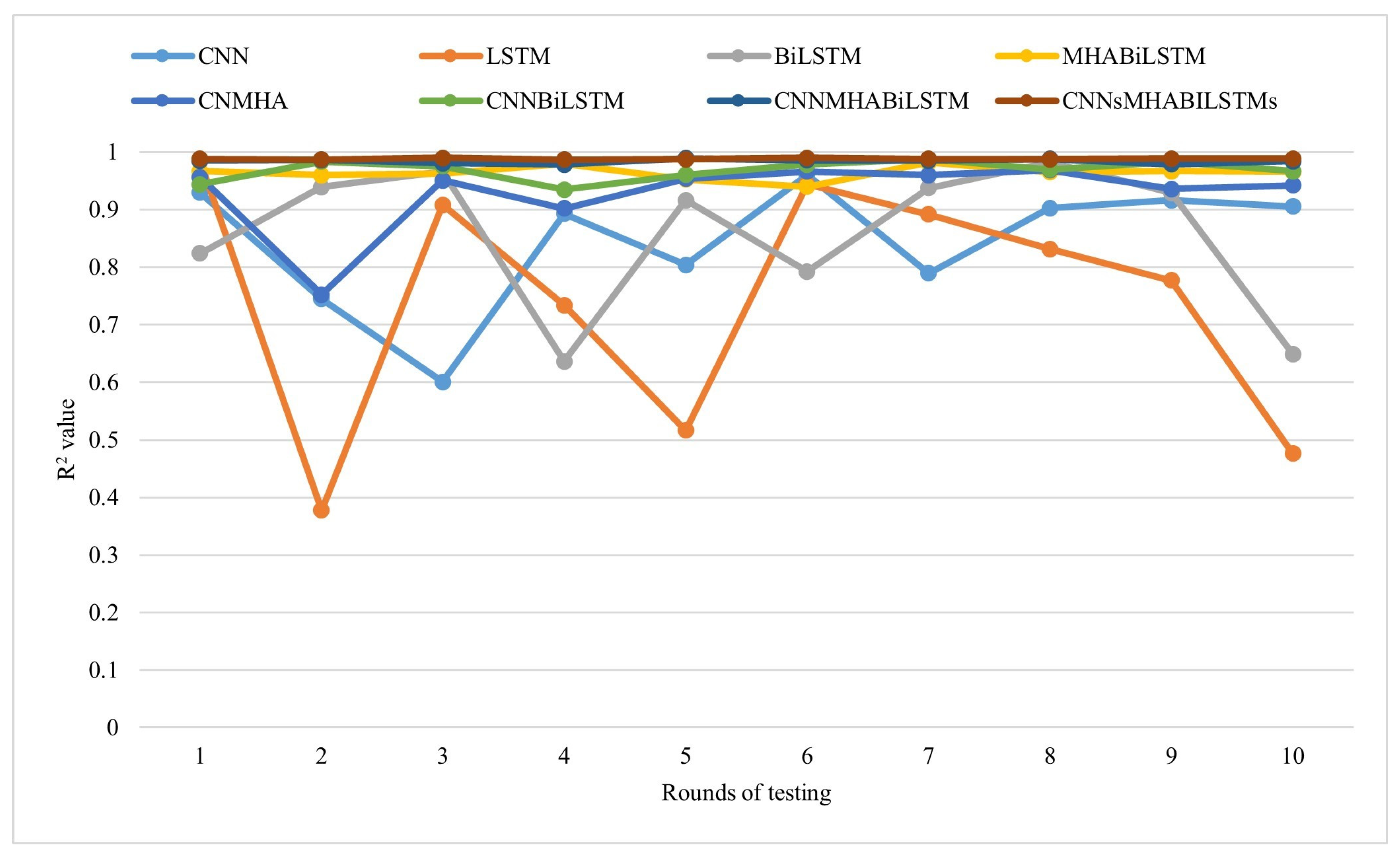
Various deep learning models (CNN, MHA, BiLSTM, and their hybrid models) were employed in this study, showing strong capabilities in processing spatiotemporal features, thereby effectively capturing the intricate patterns and characteristics present within the datasets.

3.4. Experimental Environment and Model Configuration

This study was conducted using an Intel Core i7-12700H CPU, NVIDIA GeForce GTX 3060 GPU, and 32 GB of RAM. The operating system was Windows 11 x64, and the software utilized was MATLAB R2024a. Training parameters included a batch size of 512, 200 training epochs, an initial learning rate of 0.001, and a dropout rate of 0.2. These configurations ensured the efficiency of the experiment and the effectiveness of model training.

3.5. Comparison of the Single-Point Flow Field Characteristics Predicted by Various Numerical Models

3.5.1. Prediction of the Single-Point Current Velocity

The acquired flow velocity data from the 10,800 temporal nodes were divided into three groups: 70% for training, 10% for validation, and 20% for testing. In addition to the CNNs–MHA–BiLSTMs model proposed in this study, seven other models were constructed as control groups for comparative ablation experiments: CNN, LSTM, BiLSTM, CNN–BiLSTM, MHA–BiLSTM, CNN–MHA, and CNN–MHA–BiLSTM. To comprehensively evaluate the performance of all models, the predictions were compared with those predicted by the MIKE21 FM, as well as with the hourly actual flow velocity data obtained from the Dasanshan current station in the computational field. The results are shown in Figure 16.

3.5.2. Prediction of the Single-Point Current Direction

Because flow velocity is a vector, the precise prediction of its direction is crucial. The current direction results predicted by the MIKE21 FM and CNNs–MHA–BiLSTM models, along with the measured current direction data, are shown in Figure 17. The RMSE, MAPE, and R² were found to be 0.0780 m/s, 3.07%, and 0.9919, respectively.

Based on the results of comparative experiments, the CNNs–MHA–BiLSTMs model proposed in this study demonstrated outstanding prediction accuracy. The differences between the results predicted by the MIKE21 FM and CNNs–MHA–BiLSTMs models were significantly reduced, particularly in the peak and valley segments of the data. At the extremum, the values predicted by the CNNs–MHA–BiLSTMs model aligned even more closely with the measured values than the numerical simulations, demonstrating the superiority of the CNNs–MHA–BiLSTMs model in handling critical data points.

3.6. Validation of the Reliability and Generalization Capability of the Numerical Models

Each model tested in the comparative experiments underwent 10 rounds of testing to minimize the impact of random factors that may arise during model training. The accuracy of each model was assessed using three evaluation metrics (MAPE, RMSE, and R²), as shown in Figure 18, Figure 19 and Figure 20, respectively. These metrics obtained from multiple experiments further validated the fact that the novel CNNs–MHA–BiLSTMs model proposed in this study had high accuracy, robust reliability, and stability. Even though there were minimal differences in the accuracy between the conventional CNN–MHA–BiLSTM model and the proposed CNNs–MHA–BiLSTMs model for single-point flow field characteristic predictions, the CNN–MHA–BiLSTM model exhibited suboptimal performance in spatiotemporal flow field evolution and point-to-plane prediction, as discussed later, thus failing to meet the precision required for engineering applications.

This study presents a comparison between the results predicted by the novel CNNs–MHA–BiLSTMs model and the measured values at a specific measurement point. To ensure comprehensive performance evaluation, a detailed analysis was conducted on the predicted results for the remaining 11 test points (as shown in Figure 8). As indicated in

Table 7. Evaluation metrics of the proposed CNNs–MHA–BiLSTMs model for other points.

Point	Longitude	Latitude	MAPE (%)	RMSE (m/s)	R2
2	121.73°	38.91°	2.926	0.0233	0.9834
3	121.78°	38.86°	1.649	0.0180	0.9901
4	121.78°	38.91°	2.500	0.0251	0.9808
5	121.75°	38.88°	1.136	0.0211	0.9864
6	121.75°	38.89°	2.173	0.0264	0.9787
7	121.76°	38.88°	1.276	0.0203	0.9875
8	121.76°	38.89°	2.589	0.0233	0.9835
9	121.71°	38.84°	2.129	0.0252	0.9807
10	121.71°	38.93°	3.048	0.0242	0.9822
11	121.80°	38.84°	2.287	0.0261	0.9793
12	121.80°	38.93°	1.493	0.0204	0.9873

, the proposed CNNs–MHA–BiLSTMs model meets the accuracy requirements for predictions at various locations (excluding the sampling points), demonstrating high reliability, precision, and robust generalization capability.

3.7. Comparison of the Two-Dimensional Flow Field Characteristics Predicted by Various Numerical Models

3.7.1. Prediction of the u Velocity Component of a Two-Dimensional Flow Field in Different Models

Unlike single-point experiments, this study focuses on predicting the two-dimensional flow field characteristics within a 10 km × 10 km area within the vicinity of Dalian Port. The current velocity data were decomposed into u and v components (where u represents the positive east direction in the geodetic coordinate system and v represents the positive north direction) to provide a detailed analysis of the flow field.

The proposed CNNs–MHA–BiLSTMs model was validated by comparing the u velocity components predicted by this model with those predicted by the MIKE21 FM and other deep learning models at five different times, and the results are shown in Figure 21. These velocity contours represent the u velocity component of the ocean current velocity in the red–green–blue (RGB) colour space, where the transition from blue to yellow represents an increase in current velocity from slow to fast, with yellow indicating faster current velocities and blue indicating slower current velocities.

Likewise, the deep-learning models were assessed based on the MAPE, RMSE, and R², and the results are summarized in

Table 8. Evaluation metrics and training times of various numerical models in predicting the u velocity components of two-dimensional flow fields.

Deep Learning Model	RMSE (m/s)	MAPE (%)	RMSE (m/s)	R2	Training Time (s)
CNNs–MHA–BiLSTMs	0.0784	4.7143	0.8718	2855	2855
CNN–MHA–BiLSTM	0.1046	7.7739	0.7739	2052	2052
CNN–BiLSTM	0.1241	16.4513	0.6381	484	484
CNN–MHA	0.1079	15.0139	0.7012	1498	1498
MHA–BiLSTM	0.1675	29.3405	0.3095	701	701
BiLSTM	0.2173	29.8842	0.2883	419	419
LSTM	0.2346	34.4286	0.2516	394	394
CNN	0.2583	38.2687	0.1116	330	330

. Despite the longer training time of the proposed CNNs–MHA–BiLSTMs model, this model exhibited superior accuracy and outperformed the other models based on the three evaluative metrics. The results of the u velocity component can intuitively assess the prediction capability of the models across the entire area as well as their accuracy in capturing the current velocity distribution and variation with respect to time. This experiment lays the foundation to further validate the practical application of the proposed CNNs–MHA–BiLSTMs model in predicting the characteristics of complex flow fields.

3.7.2. Prediction of the u Velocity Component of the Two-Dimensional Flow Field for Different Numbers of Sampling Points

The number of sampling points plays a pivotal role in the reconstruction of the two-dimensional flow field. In general, the greater the number of available sampling points, the more precise the reconstruction of the two-dimensional flow field. This is attributed to the fact that a larger number of sampling points provides detailed insight into the flow field, yielding a more accurate depiction of the flow field characteristics across the entire area.

Nevertheless, in practical applications, such as searching and monitoring drifting objects in oceans and USV swarm control in oceans, acquiring a large number of datasets may be an arduous task. To achieve precise reconstruction of the flow field with a limited number of sampling points, it is imperative to devise methods for optimizing the number of sampling points while simultaneously ensuring high prediction accuracy. This section focuses on the minimum number of sampling points required to accurately reconstruct the two-dimensional flow field. The minimal number of sampling points required to achieve a specific level of accuracy was determined by systematically analyzing the effect of varying the number of sampling points on the accuracy of the two-dimensional flow field reconstruction. The findings of this study will contribute to the existing body of knowledge pertaining to optimizing deployment strategies for flow measurement devices, enhancing data collection efficiency, and improving the monitoring of flow fields in practical applications.

In the preceding section, eight sampling points were used, and the results showed that the CNNs–MHA–BiLSTMs model achieved high prediction accuracy. Hence, in this section, the number of sampling points for the CNNs–MHA–BiLSTMs model varied at 4, 8, and 12 points, and the two-dimensional flow fields produced were compared with those obtained using the MIKE21 FM, as shown in Figure 22. It can be observed that the prediction accuracy was unsatisfactory, and the two-dimensional flow field exhibited significant errors when only four sampling points were used. This can be attributed to the insufficient number of sampling points and the CNNs–MHA–BiLSTMs model, which failed to fully capture the flow field characteristics, resulting in significant deviations in the two-dimensional flow field reconstructed by the CNNs–MHA–BiLSTMs and MIKE21 FM. The prediction accuracy showed a marked improvement when the number of sampling points increased. When eight sampling points were used, the two-dimensional flow field predicted by the CNNs–MHA–BiLSTMs model closely resembled those predicted by the MIKE21 FM, and the errors notably decreased, as indicated by

Table 9. Evaluation metrics and training time of the CNNs–MHA–BiLSTMs model for different numbers of sampling points.

Number of Sampling Points	RMSE (m/s)	MAPE (%)	R2	Training Time (s)
12	0.0762	3.2021	0.9029	3178
8	0.0784	4.7143	0.8718	2855
4	0.1046	9.4568	0.7566	2653

. This suggests that eight sampling points are adequate to produce an accurate reconstruction of the two-dimensional flow field. Increasing the number of sampling data points to 12 only resulted in a marginal improvement in the prediction accuracy, which may be negated by the higher computational complexity.

Following the experimental analysis outlined above, the use of eight sampling points can reduce the costs of data collection and processing while ensuring high prediction accuracy. Increasing the number of sampling points to 12 resulted in only a marginal improvement in the prediction accuracy, and the additional computational costs for data collection and processing negated the slight increase in prediction accuracy. Eight sampling points can provide comprehensive data on flow speed and direction, enabling the precise interpretation of complex aquatic conditions. A well-distributed sample point arrangement can effectively minimize errors associated with simplified flow field models. By capturing global flow features with fewer sampling points, the reliance on high-density data and processing times decreased, allowing computational resources to be concentrated on key areas, thus enhancing efficiency.

3.7.3. Prediction of the Velocity Vectors of a Two-Dimensional Flow Field

The u and v velocity components were combined to form two-dimensional ocean surface flow fields at five different times, as shown in Figure 23. The velocities predicted by the proposed CNNs–MHA–BiLSTMs model were compared to those predicted by the MIKE21 FM, and the results revealed that the velocities predicted by the CNNs–MHA–BiLSTMs model closely approximated the numerical simulation values. The proposed CNNs–MHA–BiLSTMs model effectively reconstructed two-dimensional flow fields that were very similar to those calculated by the MIKE21 FM based on only eight sampling points. The high accuracy of the two-dimensional flow field reconstruction indicates that the proposed CNNs–MHA–BiLSTMs model has exceptional generalization ability and precision, thereby validating its effectiveness and providing a reliable basis for practical applications.

3.7.4. Verification of the Two-Dimensional Flow Field Reconstruction

In this study, the prediction results across an area were visualized, as described in the preceding section. The results predicted by the CNNs–MHA–BiLSTMs and MIKE21 FM at three random points were also compared, as shown in Figure 24 with (a), (b), and (c). These red dots in the upper-right corner of the figure correspond to the geographic coordinates shown in

Table 10. Evaluation metrics and training time of the CNNs–MHA–BiLSTMs model.

Validation Point	Longitude	Latitude	RMSE (m/s)	MAPE (%)	R2
a	121.72° E	38.89° N	0.2536	12.78	0.9960
b	121.74° E	38.87° N	0.2252	19.42	0.9868
c	121.78° E	38.86° N	0.1763	13.48	0.9945

. These points lie outside the defined region enclosed by the eight sampling points, thereby serving as a test to evaluate the generalization capability of the models. It is evident that the results predicted by the CNNs–MHA–BiLSTMs and MIKE21 FM were nearly coincident, indicating very good agreement. The evaluation metrics for these points are shown in Table 10.

3.8. Result

Our proposed deep learning model demonstrates superior performance in single-point prediction, with coefficients of R² above 0.97, RMSE less than 0.03 m/s, and MAPE below 5%. The model not only significantly outperforms other comparative models in terms of stability and accuracy but also exhibits excellent robustness in practical applications. Compared to studies reconstructing the flow field based on only eight data points, our model maintains R² above 0.85, RMSE less than 0.1 m/s, and MAPE still within 5%. Although the training time for our model is relatively longer, its accuracy is markedly superior to other models. Furthermore, by comprehensively considering various factors, we determined that setting the number of data sampling points to eight during flow field reconstruction yields the highest cost-effectiveness. This configuration ensures prediction accuracy while significantly reducing data collection and processing costs, making the model more suitable for real-world applications.

4. Discussion

In this section, we discuss the benefits of flow field reconstruction and prediction in the path planning of USVs, the trajectory prediction of drifting objects and the protection of offshore structures.

In USV path planning, accurately reconstructing a real-time flow field enhances situational awareness, optimizing routes and maneuvers [28]. Dynamic updates based on real-time ocean changes improve adaptability. An accurate model can help USVs choose optimal routes, avoid energy consumption in counter currents and shorten travel times. Fast flow field reconstruction allows for quick adjustments to routes during sudden events, ensuring safety. Accurate flow data also support collaborative operations, enabling synchronized coordination among multiple USVs.

For the trajectory prediction of drifting objects, accurately reconstructing the flow field improves the precision of predicting the movement of objects in the ocean [29]. Real-time data enable rescue teams to design efficient search routes, minimizing time with resources and allowing for dynamic strategy adjustments to enhance search effectiveness. Comprehensive data support scientific rescue decisions, making them more rational. Real-time flow prediction quickly identifies threats such as pollution or collisions. These benefits collectively enhance search and rescue operations, improving monitoring and response to drifting objects in the ocean.

Accurate flow field reconstruction and prediction are crucial for ensuring the safety of marine structures [30]. By providing prediction data on flow conditions, this technology can help prevent structural failures and minimize damage from extreme weather or unexpected currents. For example, offshore platforms, buoys, and underwater installations can benefit from precise flow data to reduce stress on critical components, extend their operational lifespan, and enhance overall durability. Additionally, real-time flow field information aids in the safe positioning and operation of marine structures, supporting efficient resource extraction and environmental monitoring activities.

Reconstructing flow fields using a limited number of sampling points has shown great potential, but the low resolution of the data restricts its effectiveness in detailed applications, necessitating significant improvements [31]. In our future research, we aim to focus on enhancing resolution through advanced algorithms and deep-learning techniques, as well as optimizing the number and distribution of sampling points [32].

Additionally, we will investigate how changes in sampling points, particularly during USV movements, impact reconstruction accuracy. This research is crucial for developing methods to dynamically predict and reconstruct flow fields in real-time while USVs are in motion [33,34]. Our goal is to achieve high-precision flow field reconstruction to better support applications such as object monitoring, offshore platform protection, and USV path planning.

5. Conclusions

This study investigates the critical role of flow reconstruction and prediction in the path planning of USVs and the trajectory forecasting of drifting objects. The core contribution is the validation of the innovative CNNs-MHA-BiLSTMs model, which demonstrates significant advantages in accurately predicting flow velocity.

Key findings from this research are given as follows:

(1)

Model performance: After the model training is completed, the CNNs-MHA-BiLSTMs model demonstrates higher accuracy and stability in predicting single-point flow speed, direction, and two-dimensional flow field characteristics compared to other deep-learning models. Compared to other deep learning methods, it also exhibits higher prediction accuracy.

(2)

Sampling efficiency: Analysis in our study on a minimum of eight sampling points is necessary to achieve high precision in flow field reconstruction. This finding optimizes data collection and processing costs, facilitating effective implementation even in scenarios with limited data availability.

(3)

Robustness and validation: We have confirmed the model’s capacity to accurately predict two-dimensional ocean surface flow fields, demonstrating its effectiveness even with a reduced number of sampling points. The inclusion of u and v velocity components further reinforces the model’s applicability in real-world scenarios.

(4)

Contributions to engineering applications: we have discussed the model’s capability to reliably support USV path planning and the trajectory prediction of drifting objects, emphasizing its effectiveness in addressing challenges posed by dynamic environments and limited data availability.

In summary, this paper introduces the CNNs-MHA-BiLSTMs model as a powerful tool for flow field reconstruction and prediction, providing valuable insights for engineering applications in complex fluid environments. This study contributes to advancing the integration of deep learning techniques with numerical simulation methods in fluid mechanics, enhancing predictive capabilities and operational efficiency in ocean engineering. Future work should focus on adapting the model to various environmental conditions and its scalability for diverse marine applications.

References

1. Feng, S.; Li, F.; Li, S. Introduction to Ocean Science; Higher Education Press: Beijing, China, 1999. [Google Scholar]
2. Martínez-Moreno, J.; Hogg, A.M.; England, M.H.; Constantinou, N.C.; Kiss, A.E.; Morrison, A.K. Global changes in oceanic mesoscale currents over the satellite altimetry record. Nat. Clim. Chang. 2021, 11, 397–403. [Google Scholar] [CrossRef]
3. Mehra, A.; Rivin, I. A Real Time Ocean Forecast System for the North Atlantic Ocean. Terr. Atmos. Ocean. Sci. 2010, 21, 211–228. [Google Scholar] [CrossRef]
4. Hersbach, H.; Bidlot, J.R. The Relevance of Ocean Surface Current in the ECMWF Analysis and Forecast System. In Proceedings of the ECMWF Workshop on Ocean-Atmosphere Interactions 2008, Reading, UK, 10–12 November 2008. [Google Scholar]
5. Liu, J. Ocean Current Forecast Model Based on Wavelet and Artificial Neural Network. J. Wuhan Univ. Technol. 2013, 37, 767–770. [Google Scholar]
6. Dong, S.C. Current Prediction Research Based on ARIMA-BP Neural Network Abstract. China Sci. Technol. Inf. 2014, 2, 86–88. [Google Scholar]
7. Lv, N.; Liang, X.; Chen, C.; Zhou, Y.; Li, J.; Wei, H.; Wang, H. A long short-term memory cyclic model with mutual information for hydrology forecasting: A Case study in the xixian basin. Adv. Water Resour. 2020, 141, 103622. [Google Scholar] [CrossRef]
8. Grossi, M.D.; Kubat, M.; Özhökmen, T.M. Predicting particle trajectories in oceanic flows using artificial neural networks. Ocean Model. 2020, 156, 101707. [Google Scholar] [CrossRef]
9. Immas, A.; Do, N.; Alam, M.R. Real-time in situ prediction of ocean currents. Ocean Eng. 2021, 228, 108922. [Google Scholar] [CrossRef]
10. Yuan, H.; Guan, Q.; Zhang, T. South Pacific current forecast based on LSTM-BP neural network. Trans. Oceanol. Limnol. 2022, 44, 10–16. [Google Scholar]
11. Tang, H.; Li, Q.; Huang, L.; Zhou, C. Runoff prediction method based on CNN deep learning and its application. Water Resour. Informatiz. 2020, 6, 37–42. [Google Scholar]
12. Ma, X.; Hu, H.; Ren, Y.F. A hybrid deep learning model based on feature capture of water level influencing factors and prediction error correction for water level prediction of cascade hydropower stations under multiple time scales. J. Hydrol. 2023, 617, 129044. [Google Scholar] [CrossRef]
13. Zhao, Z.; Yang, Z. Flow Velocity Prediction Method Based on Deep Learning. In Proceedings of the Seventh International Conference on Traffic Engineering and Transportation System (ICTETS 2023), Chongqing, China, 22–24 September 2023; p. 130640. [Google Scholar]
14. Zheng, X.; Peng, Z.; Cao, Y.; Shan, H.; Zhang, J. VIP-Mixer: A Convolutional Mixer for Video Prediction. arXiv 2024, arXiv:2311.11683. [Google Scholar] [CrossRef]
15. Chen, J.; Zheng, L.; Hu, Y.; Wang, W.; Zhang, H.; Hu, X. Traffic Flow matrix-based graph neural network with attention mechanism for traffic flow prediction. Inf. Fusion 2024, 104, 102146. [Google Scholar] [CrossRef]
16. DHI. MIKE 21 & MIKE 3 Flow Model FM Hydrodynamic and Transport Module Scientific Documentation; DHI: Hørsholm Denmark, 2017. [Google Scholar]
17. Darwish, M.S.; Moukalled, F. TVD schemes for unstructured grids. J. Heat. Mass. Transf. 2023, 46, 599–611. [Google Scholar] [CrossRef]
18. Krizhevsky, A.; Sutskever, I.; Hinton, G.E. ImageNet Classification with Deep Convolutional Neural Networks. Commun. ACM 2017, 60, 84–90. [Google Scholar] [CrossRef]
19. Vaswani, A.; Shazeer, N.; Parmar, N.; Uszkoreit, J.; Jones, L.; Gomez, A.N.; Kaiser, L.; Polosukhin, I. Attention Is All You Need. In Proceedings of the 31st Conference on Neural Information Processing Systems (NIPS 2017), Long Beach, CA, USA, 4–9 December 2017. [Google Scholar]
20. Hochreiter, S.; Schmidhuber, J. Long short-term memory. Neural Comput. 1997, 9, 1735–1780. [Google Scholar] [CrossRef]
21. Siami-Namini, S.; Tavakoli, N.; Namin, A.S. The Performance of LSTM and BiLSTM in Forecasting Time Series. In Proceedings of the 2019 IEEE International Conference on Big Data, Los Angeles, CA, USA, 9–12 December 2019. [Google Scholar] [CrossRef]
22. Geernaert, G.L.; Plant, W.L. Surface Waves and Fluxes. Volume 1 Current Theory; Springer Science & Business Media: Berlin, Germany, 2013. [Google Scholar]
23. Available online: https://xihe-energy.com/#climate (accessed on 3 May 2024).
24. Liu, H. Study of The Distribution Characteristics of Current in Dalian Bay. Mar. Sci. 1990, 6, 23–27. [Google Scholar]
25. Mo, Z.; Shi, M.; Lv, Y.; Song, J.; Shang, Q. Wave hindcast simulation based on SWAN-MIKE21 nested model in an engineering area in Dalian Bay. China Harb. Eng. 2021, 41, 20–23. [Google Scholar] [CrossRef]
26. Tan, X. Study on the Total Amount Control of Pollutants Based on Environmental Capacity—A Case Study in Dalian Bay. Master’s Thesis, Dalian University of Technology, Dalian, China, 2022. [Google Scholar]
27. Available online: https://oceanknowledge.nmdis.org.cn/web/zhuanti_tide_new.view (accessed on 3 October 2024).
28. Oplapoju, O.M. Autonomous ships, port operations, and the challenges of African ports. Marit. Technol. Res. 2023, 5, 260194. [Google Scholar] [CrossRef]
29. Kim, J.C.; Yu, D.H.; Sim, J.; Son, Y.T.; Bang, K.Y.; Shin, S. Validation of OpenDrift-Based Drifter Trajectory Prediction Technique for Maritime Search and Rescue. J. Ocean Eng. Technol. 2023, 37, 145–157. [Google Scholar] [CrossRef]
30. Wang, P.; Tian, X.; Peng, T.; Lou, Y. A review of the state-of -the-art developments in the field monitoring of offshore structures. Ocean Eng. 2018, 147, 147–164. [Google Scholar] [CrossRef]
31. Caraccio, P.; Marseglia, G.; Lauria, A.; Giorgi, M.G.D. A novel deep learning approach for flow field prediction around airfoils leveraging computational space representation. Phys. Fluids 2024, 36, 107120. [Google Scholar] [CrossRef]
32. Gao, H.; Qian, W.; Dong, J.; Liu, J. Machine learning-based reduced-order reconstruction method for flow fields. Energy Build. 2024, 320, 114575. [Google Scholar] [CrossRef]
33. Sang, Q.; Tian, Y.; Jin, Q.; Yu, J. A path planning strategy for marine vehicles based on deep reinforcement learning and da-ta-driven dynamic flow fields prediction. In Proceedings of the 2021 6th International Conference on Automation, Control and Robotics Engineering (CACRE), Dalian, China, 15–17 July 2021; pp. 466–471. [Google Scholar] [CrossRef]
34. Jin, Q.; Tian, Y.; Zhan, W.; Sang, Q.; Yu, J.; Wang, X. Dynamic Data-Driven Application System for Flow Field Prediction with Autonomous Marine Vehicles. J. Mar. Sci. Eng. 2023, 11, 1617. [Google Scholar] [CrossRef]
Figure 1. Architecture of the CNNs–MHA–BiLSTMs model.
Jmse 12 01929 g001
Figure 2. Basic framework and structure of the study scheme.
Jmse 12 01929 g002
Figure 3. Dalian Port shoreline electronic nautical chart and bathymetric map of the sampling area.
Jmse 12 01929 g003
Figure 4. Two-dimensional unstructured meshes used for discretization of the computational domain in Dalian.
Jmse 12 01929 g004aJmse 12 01929 g004b
Figure 5. Water depth distribution and flow velocity vectors of the computational domain in Dalian.
Jmse 12 01929 g005
Figure 6. Tide height chart for Laohutan from 15 January 2024 (08:00) to 16 January 2024 (08:00).
Jmse 12 01929 g006
Figure 7. Current speed chart for Dasanshan Channel from 15 January 2024 (08:00) to 16 January 2024 (08:00).
Jmse 12 01929 g007
Figure 8. Current direction chart for the Dasanshan Channel from 15 January 2024 (08:00) to 16 January 2024 (08:00).
Jmse 12 01929 g008
Figure 9. Lianyungang shoreline electronic nautical chart and bathymetric map of the sampling area.
Jmse 12 01929 g009
Figure 10. Two-dimensional unstructured meshes used for discretization of the computational domain in Lianyungang.
Jmse 12 01929 g010
Figure 11. Water depth distribution and flow velocity vectors of the computational domain in Lianyungang.
Jmse 12 01929 g011
Figure 12. Tide height chart for Lianyungang from 9 April 2024 (00:00) to 10 April 2024 (00:00).
Jmse 12 01929 g012
Figure 13. Current speed chart for Lianyungang from 9 April 2024 (00:00) to 10 April 2024 (00:00).
Jmse 12 01929 g013
Figure 14. Current direction chart for Lianyungang from 9 April 2024 (00:00) to 10 April 2024 (00:00).
Jmse 12 01929 g014
Figure 15. The 10 km × 10 km area selected for model training and testing purposes.
Jmse 12 01929 g015
Figure 16. Comparison of single-point current velocity prediction results in Dasanshan.
Jmse 12 01929 g016
Figure 17. Comparison of the single-point current direction prediction results in Dasanshan.
Jmse 12 01929 g017
Figure 18. Comparison of the MAPE for each numerical model obtained from 10 rounds of testing.
Jmse 12 01929 g018
Figure 19. Comparison of the RMSE for each numerical model obtained from 10 rounds of testing.
Jmse 12 01929 g019
Figure 20. Comparison of the R2 for each numerical model obtained from 10 rounds of testing.
Jmse 12 01929 g020
Figure 21. Comparison of the u velocity component of two-dimensional flow fields predicted by various deep learning models.
Jmse 12 01929 g021
Figure 22. Comparison of the u velocity component of two-dimensional flow fields predicted by the CNNs–MHA–BiLSTMs model for different numbers of sampling points and those calculated by the MIKE21 FM.
Jmse 12 01929 g022
Figure 23. Comparison of velocity vectors of the two-dimensional flow field predicted by the CNNs–MHA–BiLSTMs and MIKE21 FM.
Jmse 12 01929 g023
Figure 24. Comparison of the results predicted by the CNNs–MHA–BiLSTMs and MIKE21 FM at three validation points.
Jmse 12 01929 g024aJmse 12 01929 g024b