Abstract
Sonar automatic target recognition (ATR) systems suffer from complex acoustic scattering, background clutter, and waveguide effects that are ever-present in the ocean. Traditional signal processing techniques often struggle to distinguish targets when noise and complicated target geometries are introduced. Recent advancements in machine learning and wavelet theory offer promising directions for extracting informative features from sonar return data. This work introduces a feature extraction and dimensionality reduction technique using the invariant scattering transform and Sparse Multi-view Discriminant Analysis for identifying highly informative features in the PONDEX09/PONDEX10 datasets. The extracted features are used to train a support vector machine classifier that achieves an average classification accuracy of 97.3% using six unique targets.
1. Introduction
Automatic target recognition (ATR) in sonar systems has long been a focal point of naval research, driven by its critical role in naval operations. Sonar targets comprise a wide range of diverse objects, spanning small objects like fish and mines to large objects such as submarines and shipwrecks. Each target presents a unique challenge for achieving low false alarm detection and high classification accuracy. The complexity of the ocean environment, caused by a combination of surface reflections, marine life, and changing ocean dynamics, complicates the traditional signal processing techniques used for separating target features from background noise. This complexity is further compounded by unknown target geometries and unknown material compositions that introduce complex scattering processes.
Designing robust algorithms for extracting and selecting features from sonar returns is thus paramount for effective automatic target recognition. Additionally, the high cost and logistical challenges associated with data collection in ocean environments makes it difficult to build large datasets of sonar returns to train machine learning-based methods. Unlike domains such as Computer Vision, where large datasets are readily available, the sonar domain is generally data starved. This increases the difficulty of training deep neural networks for detection and classification, further emphasizing the need for designing efficient and robust ATR algorithms. The focus of this work is thus to design robust machine learning algorithms that work on limited data and can generalize well to unseen data.
2. Related Work
Building automated and robust sonar target recognition systems is crucial for the detection and classification of unexploded ordinances (UXOs). In earlier efforts, statistical signal processing techniques were used, which relied on simplified probability distribution assumptions to model the data [1,2]. With the increase in labeled data and computing power, there has been a notable shift towards data-driven models over traditional statistical approaches [3]. Supervised learning algorithms, such as support vector machines (SVMs) and neural networks (NNs), have risen to prominence due to their ability to generalize well to complex acoustic datasets when provided with sufficient data [3]. However, many data-driven classifiers suffer from the “curse of dimensionality”, which is often a problem in ATR because the dimensionality of the data often exceeds the number of samples available. To circumvent this issue, many algorithms include a feature extraction and dimensionality reduction step to construct a salient feature representation that provides separation between classes [4].
One of the less well-known dimensionality reduction techniques is Canonical Correlation Analysis (CCA), a statistical technique for finding linear relationships between highly correlated features between two sets (views) of multi-dimensional variables [5]. CCA uses these two views to find pairs of basis vectors that maximizes the correlation between these two views when projected onto the basis vectors [6]. CCA has been shown to be useful for finding correlations between two channel returns to improve mine detection in synthetic aperture sonar (SAS) images [7,8]. CCA has also been employed for extracting the dominant correlations between consecutive sonar ping returns [9,10,11]. The correlations extracted from consecutive sonar ping returns have been shown to significantly improve classification accuracy when the projections are used as training data instead of the raw returns [11]. Others have used CCA for detecting changes in aligned SAS images that were taken at different times [12].
While CCA is suitable for finding linear correlations between two sets of measurements, it is unable to find relationships between multiple views simultaneously. This could be problematic for tasks where multiple sonar returns are collected or multiple decision rules need to be considered. Williams et al. avoided a multi-view correlation computation by fusing multiple sonar acoustic color images into a single acoustic color image using a Gaussian weighting function [13]. A multi-view classification approach for an object scanned at different angles was formulated with a rule-based decision fusion strategy using a weighted sum of the individual classification decisions [14]. Others have used a multi-stage classification pruning process [15] and Bayesian Data Fusion schemes for seabed classification [16]. Deep convolutional networks have also be used to learn how to combine multiple views [17]. Recently, multi-view techniques such as Multi-View Discriminant Analysis [18] have been proposed for extending CCA to multiple views while also finding linear relationships between the views that maximizes separation between classes.
Included in many sonar target recognition systems is a feature extraction step that separates highly informative features in the sonar ping response. Localized transforms such as Scale-Invariant Feature Transform (SIFT) features and wavelets are commonly used to better capture instantaneous changes in a signal. In [19], SIFT features of simulated 3D submarine models projected onto a 2D image were used as a template library for a nearest neighbor classifier. In addition to SIFT features, another popular localized feature extraction technique in the sonar literature is decomposing a signal into a wavelet basis using the Gabor wavelet [20,21]. The 1D Gabor wavelet, given by
possesses several interesting properties, such as being localized in both time (spatial) and frequency domains [22]. In this wavelet, controls the width of the Gaussian envelope and controls the periodicity of the wavelet. Gabor wavelets have been used to form a compact dictionary that separates the components of a sonar pulse [23,24,25]. A recent paper by [26] developed a feature extraction pipeline that utilized a 2D Gabor wavelet filter to separate overlapping features in acoustic color magnitude images. Additionally, recent discoveries in deep learning have revealed that many of the deep convolutional neural networks, which attain state-of-the-art results on classification image tasks, fundamentally learn wavelet representations in their initial few layers [27]. This fact is bolstered by the work of Bruna and Mallet, which showed that state-of-the-art handwritten character recognition could be achieved using an invariant scattering transform [28]. This transform uses an alternating cascade of wavelet convolution operations and the nonlinear modulus operator on the complex-valued signal and possesses many desirable properties, such as being stable to deformations and additive noise. The wavelets used in the invariant scattering transform are not learned from data but instead are predefined Morlet wavelets. The invariant scattering transform has proven its efficacy in synthetic aperture radar (SAR) automatic target recognition, achieving an impressive average accuracy of 97.63% on benchmark datasets [29].
With the emergence of deep learning, a feature extraction step is no longer necessary, as an ample supply of data allows for robust feature representations to be learned in an end-to-end deep learning pipeline. Recently, convolutional neural networks (CNNs) have been used for object classification in synthetic aperture sonar (SAS) images using clever data augmentation strategies and adaptive weight initialization schemes [30,31]. Additionally, CNNs have been used for classifying different ship types based on ship trajectory images [32]. Other studies have focused on incorporating temporal attention into CNN-based underwater target recognition systems to extract nonlinear temporal features from ship-radiated acoustic data [33]. Furthermore, previous research has proposed transformer architectures for seabed sediment classification [34] and CNN-based classifiers with an additional attention mechanism for identifying different types of ship-radiated noise [35]. Self-organizing Feature Map neural networks have been used for seabed classification using acoustic backscattering strength data with classification accuracy in the 90% range [36]. CNNs have also been used for end-to-end object detection and have achieved impressive results using simple data augmentation methods [37,38]. When collecting SAS images, sometimes the same object can be viewed multiple items from varying perspectives. Williams, et al. proposed a technique for fusing multiple SAS views of an object into one view, followed by a neural network to classify the new view [39]. While neural networks have been proven useful for many sonar applications, it is often beneficial to add constraints to the model to limit the search space and prevent overfitting. It was shown in [40] that CNNs could achieve a classification accuracy rate of SAS images on par with a human expert by simply reducing the number of filters in each convolution block and increasing the depth of the network. Another study has shown that using small neural networks can reduce the risk of overfitting when classifying fish images in underwater environments, especially when the sample size is limited [41]. Transfer Learning has also been shown to improve classification accuracy of SAS images [42,43]. The idea of Transfer Learning is to start with a deep neural network, such as VGGnet [44] or GoogLeNet [45], that has been trained to classify generic images and retrain the network to classify domain-specific images, such as SAS images. Additionally, recent work has focused on designing wavelet convolution layers where only the parameters of the wavelet need to be learned [46]. This approach of only learning the parameters of wavelets is supported by a rigorous mathematical framework from Stéphane Mallat that shows CNNs learn the hierarchical structure of images in a way that resembles wavelets [47].
One of the final steps in many machine learning pipelines is a dimensionality reduction step that picks out features that are highly correlated with the class label. Some form of dimensionality reduction is usually required for high-dimensional data due to the “curse of dimensionality” [48]. Building a classifier that works in high dimensions is a non-trivial task because data points become equidistant from each other [48]. Luckily for many applications, the data points live on a lower-dimensional manifold, which means only a subset of the total features are relevant for classification [49]. Techniques that rely on Mutual Information for selecting features in SAS images have been shown to produce a compact subset of relevant features that improve classification performance [50]. One of the more well-known dimensionality reduction techniques is Principal Component Analysis (PCA) [51]. PCA is limited to finding only linear correlations in the data. Nonlinear extensions of PCA that utilize the “kernel-trick” of support vector machines have been proposed [52]. Kernel PCA requires the kernel to be chosen ahead of time, which often results in a brute-force search over a set of potential kernels. Recently, autoencoders have replaced Kernel PCA in popularity and have shown success in finding low-dimensional representations of sonar backscattering images [53].
When performing dimensionality reduction, it is often advantageous to use as few features as possible when projecting the data into a lower-dimensional space. Using fewer features can help improve the interpretability of a model and can improve the lower-dimensional representation by removing noisy features. The naive approach to finding a subset of features that minimizes some objective function is to search through all combinations of features for the optimal subset. This combinatorial approach quickly becomes intractable as the dimensionality of the data grows. While finding a sparse set of features that minimizes some objective may seem impossible, the past few decades have seen huge gains in efficient algorithms that promote sparsity in the solution by incorporating a penalty term. One of the more well-known sparse algorithms is the least absolute shrinkage and selection operator (LASSO), which adds an penalty to ordinary least squares [54]. Since LASSO tends to encourage sparsity in the solution, the resulting predictors are usually more interpretable since only a few of the values are non-zero. More recently, feature selection algorithms that use the norm given by
where have been proposed [55]. The norm is preferable to the commonly used Frobenius norm because it is less sensitive to outliers and tends to promote sparsity along the rows of the matrix in Equation (2). The norm has been used to improve the robustness of regression tasks [55] and Principal Component Analysis [56]. Additionally, the norm has been incorporated into eigenvalue problems for selecting sparse discriminative features from a dataset [57].
3. Key Contributions
This work presents a sparse multivariate, multi-view statistical technique that selects discriminating features from nonlinear wavelet coefficients in backscattering measurements, thus revealing salient target features partially hidden in background noise. The nonlinear wavelet coefficients are computed using the invariant scattering transform, which uses a cascade of wavelets and the nonlinear modulus operator to compute a representation that is stable to additive noise and deformations. The invariant scattering transform mimics convolutional neural networks in its use of convolutional filters and nonlinear functions, but does not require us to compute a non-convex optimization problem. Trying to solve non-convex problems on small samples sizes is prone to bad solutions that fall into a poor local minima. Removing the need for ill-posed optimization problems in favor of a more deterministic approach can lead to more robust algorithms and improve interpretability of the solution. Multiple sets of robust scattering coefficients are then used as input into our proposed Sparse Multi-view Discriminant Analysis method. Sparse Multi-view Discriminant Analysis is able to find discriminating features across multiple sets of variables, similar to how Canonical Correlation Analysis can extract linear correlations between two sets of variables and Linear Discriminant Analysis finds linear combinations of features that increase the separation between classes. Additionally, a sparsity penalty is added to the multi-view discriminant, such that noisy and uninformative features are removed from the solution. The sparse solution is computed using an iterative algorithm that rapidly converges to an optimal solution. The amount of sparsity can be tuned, such that high classification accuracy can be achieved with limited features. Using these robust features, a support vector machine is trained as the classifier because it solves an efficient convex optimization problem.
The aim of this work is to build upon the existing research on wavelets and deep learning, ensuring that the results are easily interpretable by practitioners and do not require extensive amounts of data to perform well. We introduce a method that extends previous approaches by incorporating wavelets and supervised learning techniques to produce interpretable classification decisions.
To summarize, the contributions in this work are as follows:
- Nonlinear feature extraction is performed on backscattering measurements using the invariant scattering transform. The resulting scattering coefficients are stable to noise and deformations, and they are easier to interpret than convolutional neural networks. Additionally, the wavelets used in the invariant scattering transform can effectively isolate instantaneous changes in the backscattering measurements that distinguish target classes.
- A multi-view discriminant method is used as a dimensionality reduction step to find linear combinations of the features across multiple sets of variables that increase the separation between classes in a shared lower-dimensional space.
- A sparsity penalty is added to the multi-view discriminant to select only the most informative features for classification. The iterative algorithm selects features using the sparsity-inducing norm, which is convex and does not require a brute-force combinatorial search over all subsets of features.
The remainder of this paper is organized as follows. The statistical techniques that are incorporated into the final algorithm and the PondEx dataset are described in Section 5. A description of the proposed algorithm is provided in Section 6. Section 7 discusses the experimental results. Concluding remarks are made in Section 8, along with directions for future work.
4. Notation
In the following mathematical derivations, lowercase letters denote scalars, bold lowercase letters denote vectors, and bold uppercase letters denote matrices. For a square matrix, , we denote as the trace operator. Given a labeled dataset with n samples, , where each sample, , has an associated class label, , represented by a positive integer, we define c as the number of classes in the dataset and as the ith class label. The mean of the labeled dataset is given by . The mean of the ith class is denoted as , where is the number of samples in the ith class, indicates that the jth sample belongs to the ith class, and the summation runs over all samples in the ith class.
For equations involving sparsity constraints, we use the scalar as a user-defined parameter to adjust the sparsity of the solution. Similarly, is used to represent the regularization parameter for matrix inversion, denoted as , where is a positive semi-definite matrix. We denote the convolution of a signal, , with a wavelet, , as . In some contexts, may be omitted for clarity.
For a multi-view dataset, where each labeled sample has multiple views, we use to denote the jth view for the kth sample. Assuming that each sample has m different views, the jth view for all n samples can be grouped into the set . Using the corresponding class labels , the mean of the ith class for the jth view can be computed as , where is the number of samples in the ith class corresponding to the jth view. The mean across all views in the ith class is given as , where is the total number of samples in the ith class over all m views. The overall mean of the multi-view dataset is given as , where is the total number of samples over all views of each class.
5. Materials and Methods
5.1. Data
To enhance the robustness of automatic target recognition systems for small targets, the acoustic scattering mechanics of simple elastic shapes have been rigorously studied [58,59,60]. Much of the research has focused on simulating the acoustic scattering of spherical shells in three different conditions: suspended in a water column, partially buried in sand, and completely buried in sand [58]. These simulation results are then compared with experimentally collected data to verify the theoretical models. For thin, air-filled spherical shells in a water column, antisymmetric Lamb-type waves significantly influence the acoustic scattering amplitude [58]. As the frequency increases, detecting waves becomes challenging due to radiation damping, which hinders the wave’s ability to traverse the shell’s perimeter and propagate back to the sensor [58].
In this work, we showcase the effectiveness of computational methods using well-understood experimental data that reflect the previously described scattering physics. However, a detailed analysis of the scattering physics for each individual small target is beyond the scope of this work. The experiments conducted in this paper utilized the PondEx09/PondEx10 datasets. PondEx09 and PondEx10 contain a variety of targets placed in a freshwater pond at the Naval Surface Warfare Center in Panama City. The datasets were collected using the rail system developed by the Applied Physics Laboratory at the University of Washington [61]. The rail system, shown in Figure 1, consisted of a mobile tower and a fixed sonar tower. Positioned on the rail system, the mobile tower contained multiple acoustic sources and receivers. The mobile tower traveled at a speed of 0.05 m/s, emitting a ping every 0.5 s. Transmissions from the movable tower consisted of a 6 ms LFM chirp centered at 16 kHz, with a bandwidth of 30 kHz. Two-dimensional “smile” images, like the one shown in Figure 2, were formed from the ping returns that were collected as the mobile tower moved along the rail system. Matched filtered backscattering measurements of the target were collected at aspect angles ranging from −80° to 80° in 20° increments and at distances of either 5 m or 10 m from the center of the rail system. Of the possible PondEx targets, we analyzed the following: an aluminum pipe 2 ft (0.61 m) long with a 1 ft (0.305 m) diameter, a solid aluminum cylinder 2 ft (0.61 m) long with a 1 ft (0.305 m) diameter, an aluminum replica of a 4 in. (10.16 cm) artillery shell, a steel replica of a 4 in. (10.16 cm) artillery shell, an 81 mm mortar, and rock #1. A breakdown of the sample size for each target class is provided in Table 1.
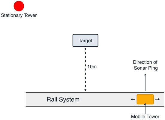
Figure 1.
Schematic diagram of the rail system used to collect data for the PondEx09/PondEx10 datasets.
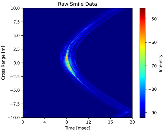
Figure 2.
A “smile” image of the steel UXO target from the PondEx dataset that was taken at 10 m with a +80° aspect angle. Values in the “smile” image are shown in decibels.

Table 1.
Number of samples per class in the PondEx09/PondEx10 datasets.
5.2. Canonical Correlation Analysis (CCA)
CCA is a statistical technique [62] that computes linear correlations between two sets of variables. The objective function of CCA aims to find a linear combination of the variables of each set that maximizes the correlation between the two sets. This is equivalent to minimizing the angle between the projected views. Specifically, let represent the first set of normalized, mean-centered variables, where each of the n columns in corresponds to an observation and each of the p rows corresponds to a variable. Similarly, let represent the second set of q normalized, mean-centered variables with the same number of observations. CCA seeks to find the coefficient vectors and , such that
is maximized, where and are the covariance matrices of and , respectively. The matrix is the cross covariance matrix between and . To guarantee that the projected variables have unit variance, the constraints
are added. We can then formulate the Lagrangian as
After solving for and in Equation (5), the two views and can be projected into a lower-dimensional space using the transformation and .
5.3. Linear Discriminant Analysis (LDA)
Linear Discriminant Analysis is a supervised statistical technique [63] that seeks to find a linear combination of features that maximally separates the means of each class while minimizing the spread of each class in the lower-dimensional space. The objective function of LDA is formulated as a Rayleigh quotient that maximizes the ratio of the between-class variance to the within-class variance.
Suppose we are given a labeled dataset of n column vectors , which have the corresponding class labels . LDA seeks to find a linear transformation matrix, , such that the Fisher Criterion [62]
is maximized, where and are the between-class scatter matrix and the within-class scatter matrix, respectively. The expressions and are the overall mean of the dataset and the mean of the samples that belong to class , respectively. Equation (6) can be rewritten as
We can then reformulate this constrained optimization problem as a non-constrained optimization problem using Lagrange multipliers
where is the trace operator and is the matrix containing the Lagrange multipliers. Taking the derivative of Equation (8) w.r.t. , we obtain
which is a generalized eigenvalue. Thus, is an eigenvector of .
5.4. Sparse LDA
Although LDA is designed to select features from high-dimensional data that maximize the separation between classes, it has no mechanism for completely eliminating noisy features that do not improve classification accuracy. Decreasing the amplitudes of the coefficients in the LDA eigenvectors that correspond to these noisy features will result in better data representations, which in turn improves classification accuracy. Our approach for producing sparse LDA eigenvectors draws inspiration from the Unsupervised Discriminate Feature Selection algorithm proposed by [57].
We again assume that we are given a labeled dataset of n column vectors , which have the corresponding class labels . Introducing sparsity into an optimization problem often involves minimizing a certain norm, such as the norm, of the vector or matrix under optimization. Maximizing Equation (6) while simultaneously minimizing a user-specified norm of matrix is a computationally difficult problem to solve efficiently. To circumvent this issue, we instead choose to minimize
which minimizes the spread of each class distribution in the lower-dimensional space while maximizing the separation between class means. The optimization in Equation (10) has the same effect as Equation (6). The problem with this approach is that is usually low rank and therefore not invertible. This can be solved by adding a regularization term, , to Equation (10)
such that . Next, to guarantee that we obtain an optimal solution, we would like to minimize a convex function. The Trace Ratio problem in Equation (11) is non-convex and cannot be solved efficiently [64]. To avoid this, we can multiply each of our training examples, , by the inverse square root of the regularized between-class scatter matrix, such that . This transformation rotates and stretches the data so that . Therefore, the new optimization that we solve is
where , since both and are positive semi-definite matrices. Now that we have an efficient way of minimizing Equation (11), we can can add a penalty to Equation (12) to promote sparsity. To accomplish this, we choose the norm, given by
where n and m are the number of rows and columns in the matrix, respectively. As demonstrated in [55], the promotes sparsity along the rows of , which leads to robust feature selection by removing individual features from all of the projection vectors in . Therefore, the objective function for this sparse LDA algorithm can be written as
where controls how sparse should be. A proof of the convergence of Algorithm A1, which is identical to the one used in [57], is included in Appendix A for completeness.
5.5. Scattering Transform
The invariant scattering transform is a signal processing technique based on wavelet theory that extracts a robust representation of an input signal using a cascade of wavelet transforms and modulus operations [28]. This technique has been applied to various tasks, such as handwritten digit recognition [28] and speech classification [65]. The combination of wavelets and the modulus has the special property of reducing variability due to translations, rotations, and arbitrary scaling, as shown in [28]. Reducing variability among target classes is crucial for robust classification, especially when dealing with small sample sizes. Additionally, the invariant scattering transform is stable to deformations, which means that small variations or distortions in the input signal will only have minor effects on the scattering coefficients. As a result, classifiers that operate on the scattering coefficients will have an easier time generalizing to unseen samples.
We will briefly review the scattering transform for completeness. Wavelets can capture multi-resolution information by scaling and rotating the mother wavelet, :
where parameterizes the scaling and rotation, j represents the change in scale, and r characterizes the rotation of the wavelet. The continuous wavelet transform, , of an input signal, , can be expressed as
The wavelet transform is not translation invariant, but instead commutes with translation. To make the transformation invariant to translations, a nonlinearity must be introduced. To make the transformation stable to deformations and additive noise, the modulus operator is chosen as the nonlinearity. The wavelet typically used in the invariant scattering transform is the complex-valued 2D Morlet wavelet, given by
where controls the drop-off of the Gaussian envelope, controls the periodicity of the complex exponential, is adjusted such that , and is the normalization constant. The scattering coefficients of the signal, x, are then calculated using the norm
While one may think that information is lost by discarding the phase of using the modulus, information is actually lost by integrating over the coefficients of . Integrating over removes all the nonzero frequencies; however, these frequencies can be recovered by computing the wavelet coefficients of , where is the wavelet used in the first “layer” and the wavelet in the second “layer” if we use the terminology commonly used in deep learning. We can continue this cascade of wavelets and modulus operators to compute a deeper representation.
To compute localized descriptors of the input signal, f, that are locally invariant to translation, a scaled spatial window function, , is used to integrate the signal locally, where controls the scale of the window function. Let be the wavelet parameters used in the invariant scattering transform. The windowed scattering transform is defined as
Using this windowed scattering transform, we can build a scattering convolution network with m layer, as shown in Figure 3.
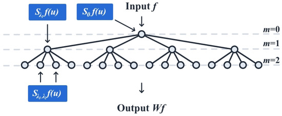
Figure 3.
Diagram of the scattering convolutional network with layers. Applying the scattering transform at the 0th layer computes the locally averaged coefficients . Applying the scattering transform at the 1st layers with the parameter computes the first-order scattering coefficients . Likewise, the outputs from the 2nd layer are computed using , where and are the parameters along a particular path in the scattering convolutional network.
Each branch in Figure 3 from the j to the layer corresponds to the rotation, r, taken from angles in . The scattering coefficients are sub-sampled after each layer in the network. The windowing function, , is also chosen to be a Gaussian.
It is important to note that, unlike conventional CNNs, the scattering convolutional network differs from the typical structure of a CNN. While conventional CNN architectures often reduce the input size through mechanisms like pooling layers and convolutional strides, this is not the case for scattering convolutional networks. Instead, scattering convolutional networks generate multiple views of the input image across various paths within the network. Each path yields scattering coefficient views that are appropriately down-sampled, ensuring that the total output dimensions from all of the scattering views remain within the same order of magnitude as the dimension of the input image.
5.6. Multi-View Discriminant Analysis (MvDA)
Multi-view Discriminant Analysis was originally proposed by Kan et. al. as a way of projecting m views into one shared lower-dimensional space by learning m projection vectors [18]. MvDA can be considered as a statistical method that combines CCA and LDA and extends them to the multi-view case. MvDA finds a shared lower-dimensional space that maximizes the ratio between between-class variation and the within-class variation, similar to Equation (6).
To compute MvDA, we assume that we are given a labeled dataset that has the corresponding labels , where is the set of samples for the jth view and is the kth sample from the jth view. The samples from the jth view are projected into the lower-dimensional space using the linear transformation . In this shared lower-dimensional space, we seek to maximize the Fisher Criterion given by
where contains the first p eigenvectors of and is the lth eigenvector that contains the projection vectors corresponding to each view. The between-class scatter matrix, , and the within-class scatter matrix, , are given as
where
is the mean over each sample of a single view in the ith class,
is the mean over all views of each sample in the ith class, and
is the mean over all views of all samples. It should also be noted that is the number of samples across all views that are in the ith class. Similarly, is the number of samples across all views of each class. The projection of the within-class scatter matrix can be reformatted in a more compact way as
where is defined as
A proof of this result is provided in Appendix A. Similarly, the between-class scatter matrix can be rewritten as
where the block element is given by
Therefore, the Fisher Criterion in Equation (20) can be expressed as
which can be solved as a generalized eigenvalue problem similar to the one solved by LDA. It is important to note that each pair of block diagonal elements and corresponds to a Fisher Criterion being computed on each of the individual views. These block diagonal elements learn intra-view discriminant information. Additionally, the off-diagonal block element pairs and compute inter-view discriminant information. This joint framework allows MvDA to learn discriminative relationships in the data across multiple views.
6. Technical Approach
The target classification pipeline employed in this paper uses a three-step approach described below to extract discriminative features and perform classification.
- Step 1: extract a robust representation of the PondEx data using an invariant scattering convolutional network described in Section 5.5.
- Step 2: project the extracted features into a lower-dimensional space using Sparse Multi-view Discriminant Analysis.
- Step 3: train an SVM classifier on the projected features.
A flow chart of the target classification pipeline is shown in Figure 4.
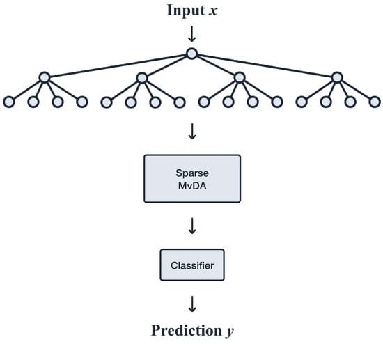
Figure 4.
Flowchart illustrating the feature extraction and features selection algorithm used for classification of the PondEx “smile” images.
6.1. Step 1: Feature Extraction Using Scattering Network
We denote each individual real-valued “smile” image in the PONDEX dataset as with its corresponding class label . The scattering convolutional network is applied to the entire “smile“ image, similar to how 2-D CNNs are used in image recognition tasks [44]. As shown in Figure 3, the scattering convolutional network does not reduce the dimensionality of the data after each layer like typical CNNs. Instead, a cascade of wavelet filters and nonlinear operators produce multiple representations of the input image. The image representation is sub-sampled after each wavelet layer, so the representation produced from a particular path in the scattering network is smaller than the original input image. However, the scattering network produces multiple views of the input image from the multiple paths. The resulting invariant scattering representation of the input has approximately the same order of magnitude of features as the original image. After applying the scattering network to the input image, , the output, , has m views for the m different sets of parameters used in the network, and each view is of size , where and . In the work, we used the Kymatio python package to compute the invariant scattering transform [66].
6.2. Step 2: Dimensionality Reduction
Prior to classification, the features extracted using the scattering network in Step 1 are projected onto a lower-dimensional subspace using MvDA. Each view in needs to be vectorized before using MvDA. We vectorize each view into a column vector using
which stacks the columns of in order. Using each training sample pair , where is the jth vectorized view of , we can construct the Multi-view Fisher Criterion in Equation (29) and solve for the eigenvectors that maximize Equation (29). After solving for the eigenvectors , the views are projected onto a subspace using the expression . The resulting vector, , and its corresponding class label can then be used to train the classifier.
As discussed in Section 5.4, it is often beneficial to enforce some constraints on an optimization problem in order to prevent overfitting to noisy features. Since MvDA is an eigenvalue problem, we can enforce sparsity by modifying the objective function. If we instead minimize the expression
We can then write the the objective function as Sparse MvDA as
where , controls the sparsity of , and controls the amount of regularization added to . Similarly, after solving for the eigenvector , the views are projected onto a lower-dimensional space using the linear equation . An SVM classifier is then trained on the robust feature vector.
6.3. Step 3: Classification
A support vector machine (SVM) was used for multi-class classification. SVMs solve a convex optimization problem and thus can be trained efficiently using custom solvers. In this work, we used the in the scikit-learn Python package [67]. SVMs are versatile classifiers because they can use the so-called “kernel trick” [68]. The kernel trick becomes beneficial when the data can be separated with a higher-order polynomial curve, but not a simple linear decision boundary. The kernel trick lifts the input data into a higher-dimensional feature space where a linear decision boundary can be drawn. We use the linear kernel to evaluate the features selected by Sparse MvDA. Additionally, if two classes overlap enough, where finding a linear decision boundary in the higher-dimensional feature space would cause overfitting, a regularization coefficient, C, can be introduced to the SVM to allow some of the data points in the training set to be misclassified. Allowing some data points in the training set to be misclassified can lead to better generalization on a holdout set. The SVM is trained on the feature vectors from PCA, MvDA, and Sparse MvDA using both the linear kernel and a small C value of 0.1. Additionally, we compare the results obtained using the invariant scattering transform with those obtained using acoustic color images. These acoustic color images are generated by applying a Blackman-windowed 8192-point Fourier Transform to each backscatter return at each cross-range position in the 2D PondEx “smile” image. The dimensionality of each image is reduced using PCA, MvDA, and Sparse MvDA individually, and each reduced image is then classified with a linear SVM with a C value of 0.1.
7. Results
7.1. Single-View Toy Example
In order to validate the design of our sparsity promoting technique, we first apply it to a toy problem where the answer is known and relatively few of the features are informative. In this example, three different class distributions are generated, which each contain 32 features, of which 4 are informative for classification. The samples for these four informative features are generated using , and the parameters of the distributions are given as
where is the mean vector of each class and is the covariance matrix for the informative features. The other 28 features are i.i.d taken from . This toy dataset serves as a good initial benchmark because it provides a controlled environment with a known ground truth, containing enough informative features to achieve robust classification results while also including a substantial number of uninformative features to effectively test the algorithm’s robustness to noisy, non-informative features.
A plot of these generated samples is shown in Figure 5. We compare both MvDA and Sparse MvDA when the number of views, m, equals 1. Having only one view means that we are effectively computing LDA and sparse LDA on the generated dataset. After minimizing the objective functions to solve for the eigenvectors, we keep the two eigenvectors corresponding to the two smallest eigenvalues. The pair of eigenvectors for MvDA and Sparse MvDA are shown in Figure 6 and Figure 7, respectively. The eigenvector pairs in Figure 6 show that the ordinary MvDA is able to pick out the four informative features, but also fits to the noisy features that do not provide any discriminative information. We can see in Figure 6 that ordinary MvDA has overfit to the training data since the three classes are perfectly separable in the training dataset but have considerable overlap in the testing set. This is not the case for Sparse MvDA, where, in Figure 7, the coefficients in the eigenvectors that correspond to noisy features are basically zero. The projections of the data in Figure 7 show that, while the projected training set is not perfectly separable, the learned eigenvectors generalize significantly better to the test set than the eigenvectors learned from ordinary MvDA.
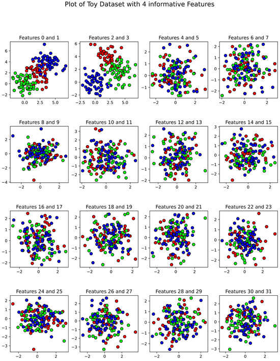
Figure 5.
Plot of the single-view toy dataset used to determine if MvDA and Sparse MvDA can select the discriminative features without overfitting to the noisy features. The three colors (red, green, and blue) in the subplots represent the three classes in this example. Features 0 to 3 provide discriminative information for classification, whereas features 4 to 31 are considered noisy features sampled from the same Gaussian distribution.
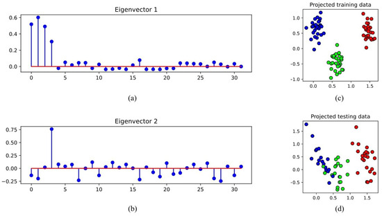
Figure 6.
The coefficients of the first two eigenvectors for MvDA are plotted in (a,b). Features 0 to 3 have larger coefficients values than the noisy features, which means MvDA was able to find the discriminative features. However, many of the coefficients for the noisy features are non-zero. The toy dataset displayed in Figure 5 was split into training and testing datasets using an 80/20 rule and projected into a lower-dimensional space using the eigenvectors in (a,b). (c) shows the training data separate into three nice clusters. However, in (d), there is significant overlap between the blue and green class clusters in the testing set.
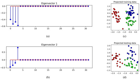
Figure 7.
The coefficients of the first two eigenvectors for Sparse MvDA are plotted in (a,b). Features 0 to 3 have larger coefficients values than the noisy features, which means Sparse MvDA was also able to find the discriminative features. However, unlike MvDA, most of the coefficients in (a,b) that correspond to the noisy features are near zero. In (c,d), we again used an 80/20 rule to split the toy dataset into a training and testing dataset. Using the first two eigenvectors in (a,b), the data are projected into a two-dimensional space. (c) shows that the training data group into three labeled clusters that only partially overlap. Additionally in (d), the clusters for the three classes overlap significantly less than the training clusters shown in Figure 6d.
We evaluate Sparse MvDA against MvDA and PCA across 10 random shuffles of the dataset described above. Sparse MvDA uses the parameters and . We use the first two components of Sparse MvDA and MvDA to project the data, as the inherent rank of in Equation (29) is determined by the three classes. For PCA, we use 14 principal components, which provide the best average classification results. After projecting the data into a lower-dimensional subspace, the data points are classified using a linear SVM with regularization parameter . The results, shown in Table 2, indicate that PCA performs the worst of the three methods. This is because PCA maximizes variance in the projection directions but does not necessarily enhance class separation, unlike MvDA and Sparse MvDA. MvDA and Sparse MvDA perform similarly, with Sparse MvDA slightly outperforming MvDA due to its added sparsity constraint, which makes it more resilient to overfitting from noisy features.

Table 2.
We evaluated the classification results across 10 random shuffles of the toy dataset shown in Figure 5. Each shuffle split the dataset into training and testing sets with a 60/40 ratio. PCA, MvDA, and Sparse MvDA were trained on the training data and used to project the data into a lower-dimensional space. Subsequently, a linear support vector machine (SVM) was employed to classify the projected data. The classification results presented below show the performance of each trained method on the test set.
7.2. Classification Accuracy on PondEx Datasets
We use the mean classification accuracy to determine how well each method performed on the PondEx dataset. Each model we compare was trained on 10 random shuffles of the dataset, where the mean classification is calculated as
where is the set of ground truth labels for each sample in the test set and is the set of predicted labels for each sample in the test set. The mean classification accuracies using PCA, MvDA, and Sparse MvDA trained on invariant scattering coefficients (an example of which is shown in Figure 8), alongside PCA, MvDA, and Sparse MvDA trained on acoustic color images, are listed in Table 3. It is evident from Table 3 that the three dimensionality reduction techniques trained on the invariant scattering coefficients outperform the classification algorithms trained on the acoustic color images. Notably, both of the supervised methods (MvDA and Sparse MvDA) and the unsupervised method (PCA) show significant improvements in classification accuracy due to this feature extraction step. This boost in performance for the PCA is especially notable, showcasing the effectiveness of the invariant scattering transform. This advantage stems from the invariant scattering transform’s ability to differentiate target classes using a combination of localized wavelets and nonlinearities.
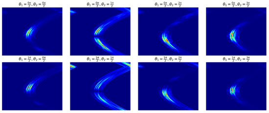
Figure 8.
Scattering coefficients of a mortar “smile” image for different paths through a scattering convolution network, similar to the network in Figure 3. The coefficients are computed according to Equation (19). Using f to represent the “smile” image, the scattering coefficients shown are obtained by varying the rotation parameter of the wavelets in , where and control the rotation and scale of the wavelet. The specific values of and are indicated for each subplot.

Table 3.
We evaluated the classification results across 10 random shuffles of the PondEx dataset, employing an 80/20 training/test split. The first three dimensionality reduction technique listed were trained on acoustic color images, as described in Section 6.3. For the last three techniques, the invariant scattering transform was first applied to extract features from PondEx images. Subsequently, the resulting invariant scattering coefficients were projected into a lower-dimensional space using one of the three techniques mentioned. Following dimensionality reduction, a linear support vector machine was employed to classify the projected data from all four listed methods.
To investigate how altering the level of sparsity impacts the mean classification accuracy of Sparse MvDA, we experiment by varying the parameter. Figure 9 and Figure 10 show classification results for parameters taken from the set . Figure 9 shows mean classification accuracy trend lines for the four different parameters using only the first 20 PCA components from each scattering coefficient view. The x-axis in Figure 9 shows the number of Sparse MvDA eigenvectors used to project the views into a lower-dimensional space. In Figure 9, a discernible trend emerges: as the number of eigenvectors increases, so does the mean classification accuracy. Moreover, it is worth noting that, when the number of eigenvectors is held constant, an increase in tends to correspond with a decrease in mean classification accuracy. The cyan line, which corresponds to , lags behind the other accuracy lines. This discrepancy is due to the parameter being too strong and eliminating too many features in the first few eigenvectors. The cyan line does eventually converge to the same mean classification accuracy as the other three curves, but it takes a significant number of eigenvectors to do so. Additionally, the red and green curves corresponding to and reach their maximum mean classification accuracy with fewer eigenvectors and remain constant as the number of eigenvectors increases. This means that an ideal that maximizes both the mean classification accuracy and the number of noisy features removed is somewhere in the range between and .
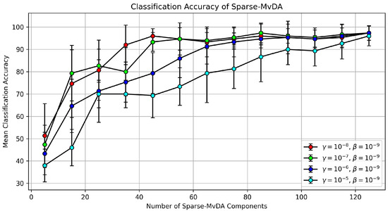
Figure 9.
Mean classification accuracy for Sparse MvDA on the PondEx dataset. The x-axis indicates the number of eigenvectors used to project the data into a lower-dimensional space prior to classification. Each colored line indicates the sparsity parameter, , used for the penalty. Each line also uses as the regularization term and the first 20 PCA components from each scattering coefficient view.
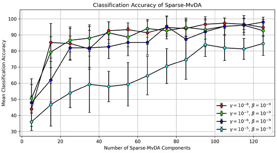
Figure 10.
Mean classification accuracy for Sparse MvDA on the PondEx dataset. The x-axis indicates the number of eigenvectors used to project the data into a lower-dimensional space prior to classification. Each colored line indicates the sparsity parameter, , used for the penalty. Each line also uses as the regularization term and the first 30 PCA components from each scattering coefficient view.
Additionally, Figure 10 shows mean classification accuracy trend lines for the four different parameters using the first 30 PCA components from each scattering coefficient view. We see that the trends for the four different parameters are similar to the ones shown in Figure 9. The cyan curves lags behind the three other curves. The separation between the curve and the three other curves is more pronounced than the gap shown in Figure 9. Additionally, the cyan curve in Figure 10 never converges to the maximum mean classification accuracy achieved by the three other curves, like was seen in Figure 10. The cyan curve settles out at about 85% mean classification accuracy. Since the models trained in Figure 10 use 30 PCA components from each scattering coefficient view instead of 20 PCA components, the curve corresponding to in Figure 10 is eliminating too many features that are needed for classification. Similar to Figure 9, the three other curves take fewer eigenvectors to reach maximum classification accuracy and also achieve a higher classification accuracy.
To evaluate the effectiveness of the invariant scattering transform at extracting the nonlinear features in the PondEx dataset, we compare different classifiers for the classification of the six targets. Since our goal is to use only the invariant scattering transform to isolate nonlinear features, we limited our analysis to linear classifiers, given the small sample size of the PondEx dataset. Before applying each classifier, we project the data into a lower-dimensional subspace using one of the following methods: Linear Discriminant Analysis (LDA), Multi-view Discriminant Analysis (MvDA), or Sparse Multi-view Discriminant Analysis (Sparse MvDA). Following this projection, the samples are classified using either a linear support vector machines or linear Logistic Regression. The results are shown in Table 4. The two classifiers achieve similar classification accuracies across each of the three projection methods, with the SVM slightly outperforming Logistic Regression, which is typical when comparing the two methods.

Table 4.
We evaluated the classification results across 10 random shuffles of the PondEx dataset, employing an 80/20 training/test split. For all listed techniques, the invariant scattering transform was first applied to extract features from PondEx images. Subsequently, the resulting invariant scattering coefficients were projected into a lower-dimensional space using one of the three techniques mentioned. Following dimensionality reduction, either a linear support vector machine or linear Logistic Regression was employed to classify the projected data from all listed methods.
To visualize the misclassification patterns, we present the classification results from Table 4 as confusion matrices in Figure 11. These confusion matrices are row normalized using the mean classification accuracy across 10 different splits. In the confusion matrix grid in Figure 11, the left column represents results using the SVM as the classifier, while the right column corresponds to Logistic Regression. The rows of the confusion matrix grid indicate the use of LDA, MvDA, or Sparse MvDA as the subspace projection method. A consistent misclassification across all confusion matrices is the mortar being incorrectly classified as rock #1. This misclassification is most pronounced when LDA is used for subspace projection. Due to the small sample size of the dataset, this misclassification is most likely caused by LDA, as well as MvDA and Sparse MvDA, not having enough samples to separate the distributions between the mortar and rock #1. Additionally, in some confusion matrices, the steel artillery shell (AL UXO Shell) is misclassified as the aluminum artillery shell (AL UXO Shell). Both the aluminium artillery shell and the steel artillery shell were originally machined from the same CAD drawing and thus have similar geometries [61], which could account for the occasional misclassification. Given the results presented in Table 4 and Figure 11, the SVM is preferable to Logistic Regression as the classifier. Additionally, while MvDA achieves the highest classification accuracy among the subspace projection methods, we can trade off a slight decrease in accuracy for greater interpretability by using Sparse MvDA.
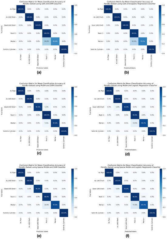
Figure 11.
Each subfigure (a–f) in the figure above presents a row normalized confusion matrices for the results shown in Table 4. In each subfigure, the x-axis represents the predicted class labels, and the y-axis represents the true class labels for the targets. Percentages along the diagonal indicate the proportion of correctly classified targets, while off-diagonal percentages represent the proportion of misclassifications for each class. In the confusion matrix grid, the left column represents the results using a support vector machine as the classifier, while the right column represents the results using Logistic Regression. The rows of the grid correspond to the subspace projection methods used: LDA, MvDA, and Sparse MvDA, listed from top to bottom.
To verify that Sparse MvDA is learning the correct features for discrimination, the magnitude of the coefficients of the eigenvector matrix are plotted in Figure 12a–c for s taken from , respectively. Plotting the magnitude of the coefficients in allows one to visually inspect how sparse the matrix is. Figure 12a shows the magnitude coefficients for when . We can see in Figure 12a that the majority of the coefficients are nearly zero, with only a few non-zero coefficients that contain most of the energy. The color bar on the right of Figure 12a shows that coefficients that appear white have a value around 0.8. Since the eigenvectors are normalized to be unit length, this means that the coefficients that appear white contain the majority of the energy of the eigenvector. Additionally, the coefficients in Figure 12a are arranged such that horizontal strips are visible. As was previously mentioned, this is a byproduct of the row sparsity property of the norm. The strips are visible because many of the non-informative features have been removed.
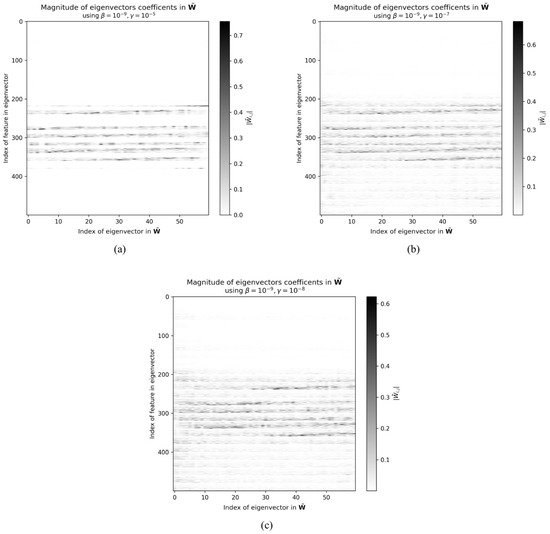
Figure 12.
The magnitude of the eigenvector coefficients in the projection matrix learned by Sparse MvDA are plotted. The first 20 PCA components from each scattering coefficient view were used, along with the regularization term and the sparsity penalties , , and . These are shown in (a–c), respectively.
Looking at Figure 12b,c, which show the magnitude coefficients for and , respectively, we see that the horizontal strip pattern is again visible. Comparing Figure 12a with Figure 12b,c, it is apparent that the energy of the eigenvectors in Figure 12a is concentrated in a fewer number of coefficients. The energy of the coefficients in Figure 12b,c are spread out across a greater number of coefficients. This is to be expected since increasing the sparsity parameter, , promotes the removal of more features in . This also explains why we see the curve in Figure 9 and Figure 10 lagging behind the other curves. By increasing to , the algorithm becomes excessively restrictive, forcing the removal of both noisy features and those critical for classification.
To achieve a suitable sparse representation, it is important to train the algorithm until it converges. A proof is provided in Appendix A, which shows the objective function in Equation (32) is a monotonically decreasing function. The minimization procedure in Algorithm A1 continues until the difference in the loss value between two successive iterations is less than a predefined threshold (we use ). Figure 13a–c show the loss curves for Sparse MvDA for values of , , and , respectively. All three curves converge to a minimum rapidly. The curve for takes the greatest number of iterations to converge (18 iterations), whereas the loss curve for in Figure 13c takes only 4 iterations to converge. Figure 13a takes more iterations because a stronger penalty is being used and thus requires more features to be eliminated for the matrix.
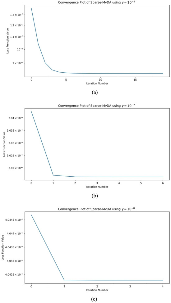
Figure 13.
Plots of the loss function in Equation (32) for Sparse MvDA using the sparsity parameters , , and , shown in (a–c), respectively.
8. Conclusions
In this work, we developed a multi-stage algorithm for extracting salient features and selecting the most discriminative features. Feature extraction was performed using the invariant scattering transform, which mimics the nonlinear feature extraction of convolutional neural networks without needing to solve a non-convex optimization problem. After feature extraction, the most discriminative features were selected using Multi-view Discriminant Analysis with a sparsity penalty. MvDA finds projection vectors that maximize the separation between class means when multiple sets of variables are projected into a shared lower-dimensional space. The additional sparsity penalty promotes row-wise sparsity of the projection matrix. Row-wise sparsity removes noisy features that negatively bias the projections of the data, which helps prevent overfitting. Using the discriminative features selected by Sparse MvDA, we achieved a mean classification accuracy of over 10 random shuffles of the data. We also demonstrated that the projection matrix learned by Sparse MvDA becomes row sparse due to the sparsity penalty. Visual inspection of the magnitude of the coefficients in shows that many of the coefficients are zero, with the non-zero coefficients being the most discriminative features. We observe that the iterative algorithm used for finding the sparse solution converges rapidly, usually taking less than 10 iterations. Additionally, we showed that using the invariant scattering transform increases the classification accuracy of both supervised and unsupervised dimensionality reduction techniques when compared with the standard acoustic color representation of sonar backscattering data.
Future steps include extending Sparse MvDA to nonlinear dimensionality reduction using the kernel method. Kernel methods allow one to project data into a higher-dimensional feature space where linear dimensionality reduction can be performed. Kernel methods would be useful if the scattering coefficients can be separated by a higher-order polynomial but not a simple linear decision boundary. This extension would be relatively straightforward since the kernel trick maps data points and to higher dimensions via their inner product. We show in the paper that MvDA can be expressed as the inner product of the data points in the training set.
Author Contributions
Conceptualization, A.S.G. and I.K.; methodology, A.C.; software, A.C.; validation, A.S.G., I.K. and A.C.; formal analysis, A.C.; investigation, A.C.; resources, A.S.G. and I.K.; data curation, A.C.; writing—original draft preparation, A.C.; writing—review and editing, A.S.G., I.K. and A.C.; visualization, A.C.; supervision, A.S.G.; project administration, A.S.G.; funding acquisition, A.S.G. All authors have read and agreed to the published version of the manuscript.
Funding
The authors would like to acknowledge the Office of Naval Research (ONR) Grant Nos. N000142112420 and N000142312503 and Department of Defense Navy (NEEC) Grant No. N001742010016 for funding of this research.
Institutional Review Board Statement
Not applicable.
Informed Consent Statement
Not applicable.
Data Availability Statement
The PONDEX09/PONDEX10 data [2,69,70] are currently available at https://www.dropbox.com/scl/fo/557eogwg5b9uvjvqe2azk/hrlkey=js0s6d0rc2hzhpvh1sez6b7mk&dl=0 (accessed on 1 June 2024). If for some reason the Dropbox link ceases to function in the future, the PONDEX09/PONDEX10 data are also available upon request from the Applied Physics Laboratory, University of Washington.
Conflicts of Interest
The authors declare no conflicts of interest.
Abbreviations
The following abbreviations are used in this manuscript:
| ATR | Automatic target recognition |
| UXOs | Unexploded ordinances |
| SAS | Synthetic aperture sonar |
| ML | Machine learning |
| CNN | Convolutional neural network |
| PCA | Principal Component Analysis |
| LDA | Linear Discriminant Analysis |
| CCA | Canonical Correlation Analysis |
| MvDA | Multi-view Discriminant Analysis |
| SVM | Support vector machine |
| NN | Neural network |
Appendix A
Appendix A.1
The following derivation shows how to reformulate the within-class scatter matrix in terms of Equation (26). We start with the definition of from Equation (21):
Here, we use Equation (23) to reduce many of the summations down to the difference from the mean. We can continue the reformation using Equation (23) again:
where is the Kronecker delta function.
Appendix A.2
| Algorithm A1: An efficient iterative algorithm to solve the sparsity optimization problem in Equation (32) |
Data: , Result: 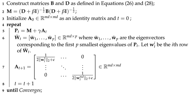 |
Lemma A1.
For any nonzero constants , the following inequality holds [55,57]
Proof.
We start with the inequality , then we have
Divide each side by
This completes the proof of Lemma A1. Now, we can substitute and with and , respectively.
Additionally, according to Lemma A1, for each row , we have
which means the following inequality holds for all i
□
Theorem A1.
In each iteration, Algorithm will monotonically decrease the objective of the problem in Equation (32).
Proof.
Using the definition of in Algorithm A1, we can see that the solution at iteration t is
This formulation indicates that each iteration of Algorithm A1 involves solving an eigenvalue problem. Consequently, the solution at each subsequent iteration satisfies the inequality
That is to say
since
Using some algebraic manipulation, we have
According to Lemma A1, , which also implies
After rearranging terms in Equation (A15), we have
Since the left-hand side of the inequality in Equation (A16) is non-negative, we therefore have the following inequality
Thus, the objective function in Equation (32) monotonically decreases using the update rule described in Algorithm A1. □
References
- Soules, M.E.; Broadwater, J.B. Featureless classification for active sonar systems. In Proceedings of the OCEANS’10 IEEE SYDNEY, Sydney, NSW, Australia, 24–27 May 2010; pp. 1–5. [Google Scholar]
- Hall, J.J.; Azimi-Sadjadi, M.R.; Kargl, S.G.; Zhao, Y.; Williams, K.L. Underwater unexploded ordnance (UXO) classification using a matched subspace classifier with adaptive dictionaries. IEEE J. Ocean. Eng. 2018, 44, 739–752. [Google Scholar] [CrossRef]
- Bianco, M.J.; Gerstoft, P.; Traer, J.; Ozanich, E.; Roch, M.A.; Gannot, S.; Deledalle, C.A. Machine learning in acoustics: Theory and applications. J. Acoust. Soc. Am. 2019, 146, 3590–3628. [Google Scholar] [CrossRef]
- Stack, J. Automation for underwater mine recognition: Current trends and future strategy. In Proceedings of the Detection and Sensing of Mines, Explosive Objects, and Obscured Targets XVI, Orlando, FL, USA, 25–29 April 2011; Volume 8017, pp. 205–225. [Google Scholar]
- Muller, K.E. Understanding canonical correlation through the general linear model and principal components. Am. Stat. 1982, 36, 342–354. [Google Scholar] [CrossRef]
- Hardoon, D.R.; Szedmak, S.; Shawe-Taylor, J. Canonical correlation analysis: An overview with application to learning methods. Neural Comput. 2004, 16, 2639–2664. [Google Scholar] [CrossRef] [PubMed]
- Wachowski, N.; Azimi-Sadjadi, M.R. A new synthetic aperture sonar processing method using coherence analysis. IEEE J. Ocean. Eng. 2011, 36, 665–678. [Google Scholar] [CrossRef]
- Tucker, J.D.; Azimi-Sadjadi, M.R. Coherence-based underwater target detection from multiple disparate sonar platforms. IEEE J. Ocean. Eng. 2011, 36, 37–51. [Google Scholar] [CrossRef]
- Yamada, M.; Cartmill, J.; Azimi-Sadjadi, M.R. Buried underwater target classification using the new BOSS and canonical correlation decomposition feature extraction. In Proceedings of the OCEANS 2005 MTS/IEEE, Washington, DC, USA, 17–23 September 2005; pp. 589–596. [Google Scholar]
- Pezeshki, A.; Azimi-Sadjadi, M.R.; Scharf, L.L. Undersea target classification using canonical correlation analysis. IEEE J. Ocean. Eng. 2007, 32, 948–955. [Google Scholar] [CrossRef][Green Version]
- Kubicek, B.; Sen Gupta, A.; Kirsteins, I. Canonical correlation analysis as a feature extraction method to classify active sonar targets with shallow neural networks. J. Acoust. Soc. Am. 2022, 152, 2893–2904. [Google Scholar] [CrossRef]
- Tesfaye, G.; Marchand, B.; Tucker, J.D.; Marston, T.M.; Sternlicht, D.D.; Azimi-Sadjadi, M.R. Image-based automated change detection for synthetic aperture sonar by multistage coregistration and canonical correlation analysis. IEEE J. Ocean. Eng. 2015, 41, 592–612. [Google Scholar]
- Williams, D.P.; España, A.; Kargl, S.G.; Williams, K.L. A family of algorithms for the automatic detection, isolation, and fusion of object responses in sonar data. In Proceedings of the Meetings on Acoustics, Virtual, 20–25 June 2021; Volume 44. [Google Scholar]
- Langner, F.A.; Jans, W.; Knauer, C.; Middelmann, W. Advantages and disadvantages of training based object detection/classification in SAS images. In Proceedings of the Meetings on Acoustics, Edinburgh, Scotland, 2–6 July 2012; Volume 17. [Google Scholar]
- Dobeck, G.J. Algorithm fusion for automated sea mine detection and classification. In Proceedings of the MTS/IEEE Oceans 2001. An Ocean Odyssey. Conference Proceedings (IEEE Cat. No. 01CH37295), Honolulu, HI, USA, 5–8 November 2001; Volume 1, pp. 130–134. [Google Scholar]
- Williams, D.P. Bayesian data fusion of multiview synthetic aperture sonar imagery for seabed classification. IEEE Trans. Image Process. 2009, 18, 1239–1254. [Google Scholar] [CrossRef]
- Miao, Y.; Zakharov, Y.V.; Sun, H.; Li, J.; Wang, J. Underwater acoustic signal classification based on sparse time–frequency representation and deep learning. IEEE J. Ocean. Eng. 2021, 46, 952–962. [Google Scholar] [CrossRef]
- Kan, M.; Shan, S.; Zhang, H.; Lao, S.; Chen, X. Multi-view discriminant analysis. IEEE Trans. Pattern Anal. Mach. Intell. 2015, 38, 188–194. [Google Scholar] [CrossRef] [PubMed]
- Zhu, Z.; Xu, X.; Yang, L.; Yan, H.; Peng, S.; Xu, J. A model-based sonar image atr method based on sift features. In Proceedings of the OCEANS 2014-TAIPEI, Taipei, Taiwan, 7–10 April 2014; pp. 1–4. [Google Scholar]
- Attaf, Y.; Boudraa, A.O.; Ray, C. Amplitude-based dominant component analysis for underwater mines extraction in side scans sonar. In Proceedings of the OCEANS 2016-Shanghai, Shanghai, China, 10–13 April 2016; pp. 1–4. [Google Scholar]
- Madhusudhana, S.; Gavrilov, A.; Erbe, C. Automatic detection of echolocation clicks based on a Gabor model of their waveform. J. Acoust. Soc. Am. 2015, 137, 3077–3086. [Google Scholar] [CrossRef]
- Mallat, S. A Wavelet Tour of Signal Processing; Elsevier: Amsterdam, The Netherlands, 1999. [Google Scholar]
- Gupta, A.S.; Schupp, D. Characterization of sonar target data using Gabor wavelet features. In Proceedings of the 2015 49th Asilomar Conference on Signals, Systems and Computers, Pacific Grove, CA, USA, 8–11 November 2015; pp. 1723–1726. [Google Scholar]
- Gupta, A.S.; Kirsteins, I. Disentangling sonar target features using braided feature graphs. In Proceedings of the OCEANS 2017-Anchorage, Anchorage, AK, USA, 18–21 September 2017; pp. 1–5. [Google Scholar]
- Gupta, A.S.; Kirsteins, I. Sonar signaling employing braid-encoded features on sparse gabor dictionaries. In Proceedings of the OCEANS 2019 MTS/IEEE SEATTLE, Seattle, WA, USA, 27–31 October 2019; pp. 1–4. [Google Scholar]
- Kubicek, B.; Sen Gupta, A.; Kirsteins, I. Sonar target representation using two-dimensional Gabor wavelet features. J. Acoust. Soc. Am. 2020, 148, 2061–2072. [Google Scholar] [CrossRef]
- Shang, W.; Sohn, K.; Almeida, D.; Lee, H. Understanding and improving convolutional neural networks via concatenated rectified linear units. In Proceedings of the International Conference on Machine Learning, PMLR, New York City, NY, USA, 19–24 June 2016; pp. 2217–2225. [Google Scholar]
- Bruna, J.; Mallat, S. Invariant scattering convolution networks. IEEE Trans. Pattern Anal. Mach. Intell. 2013, 35, 1872–1886. [Google Scholar] [CrossRef]
- Wang, H.; Li, S.; Zhou, Y.; Chen, S. SAR automatic target recognition using a Roto-translational invariant wavelet-scattering convolution network. Remote Sens. 2018, 10, 501. [Google Scholar] [CrossRef]
- Williams, D.P. Underwater target classification in synthetic aperture sonar imagery using deep convolutional neural networks. In Proceedings of the 2016 23rd International Conference on Pattern Recognition (ICPR), Cancun, Mexico, 4–8 December 2016; pp. 2497–2502. [Google Scholar]
- Wang, X.; Jiao, J.; Yin, J.; Zhao, W.; Han, X.; Sun, B. Underwater sonar image classification using adaptive weights convolutional neural network. Appl. Acoust. 2019, 146, 145–154. [Google Scholar] [CrossRef]
- Yang, T.; Wang, X.; Liu, Z. Ship type recognition based on ship navigating trajectory and convolutional neural network. J. Mar. Sci. Eng. 2022, 10, 84. [Google Scholar] [CrossRef]
- Jin, A.; Zeng, X. A novel deep learning method for underwater target recognition based on res-dense convolutional neural network with attention mechanism. J. Mar. Sci. Eng. 2023, 11, 69. [Google Scholar] [CrossRef]
- Wang, H.; Zhou, Q.; Wei, S.; Xue, X.; Zhou, X.; Zhang, X. Research on seabed sediment classification based on the MSC-transformer and sub-bottom profiler. J. Mar. Sci. Eng. 2023, 11, 1074. [Google Scholar] [CrossRef]
- Liu, D.; Yang, H.; Hou, W.; Wang, B. A Novel Underwater Acoustic Target Recognition Method Based on MFCC and RACNN. Sensors 2024, 24, 273. [Google Scholar] [CrossRef] [PubMed]
- Zhao, J.; Zhang, H. Seabed classification based on sofm neural network. In Proceedings of the 2008 International Conference on Computer Science and Software Engineering, Wuhan, China, 12–14 December 2008; Volume 4, pp. 902–905. [Google Scholar]
- Valdenegro-Toro, M. End-to-end object detection and recognition in forward-looking sonar images with convolutional neural networks. In Proceedings of the 2016 IEEE/OES Autonomous Underwater Vehicles (AUV), Tokyo, Japan, 6–9 November 2016; pp. 144–150. [Google Scholar]
- Nguyen, H.T.; Lee, E.H.; Lee, S. Study on the classification performance of underwater sonar image classification based on convolutional neural networks for detecting a submerged human body. Sensors 2019, 20, 94. [Google Scholar] [CrossRef]
- Williams, D.P.; Dugelay, S. Multi-view SAS image classification using deep learning. In Proceedings of the OCEANS 2016 MTS/IEEE Monterey, Monterey, CA, USA, 19–23 September 2016; pp. 1–9. [Google Scholar]
- Williams, D.P. On the use of tiny convolutional neural networks for human-expert-level classification performance in sonar imagery. IEEE J. Ocean. Eng. 2020, 46, 236–260. [Google Scholar] [CrossRef]
- Paraschiv, M.; Padrino, R.; Casari, P.; Bigal, E.; Scheinin, A.; Tchernov, D.; Fernández Anta, A. Classification of underwater fish images and videos via very small convolutional neural networks. J. Mar. Sci. Eng. 2022, 10, 736. [Google Scholar] [CrossRef]
- McKay, J.; Gerg, I.; Monga, V.; Raj, R.G. What’s mine is yours: Pretrained CNNs for limited training sonar ATR. In Proceedings of the OCEANS 2017-Anchorage, Anchorage, AK, USA, 18–21 September 2017; pp. 1–7. [Google Scholar]
- Jin, L.; Liang, H.; Yang, C. Accurate underwater ATR in forward-looking sonar imagery using deep convolutional neural networks. IEEE Access 2019, 7, 125522–125531. [Google Scholar] [CrossRef]
- Simonyan, K.; Zisserman, A. Very deep convolutional networks for large-scale image recognition. arXiv 2014, arXiv:1409.1556. [Google Scholar]
- Szegedy, C.; Liu, W.; Jia, Y.; Sermanet, P.; Reed, S.; Anguelov, D.; Erhan, D.; Vanhoucke, V.; Rabinovich, A. Going deeper with convolutions. In Proceedings of the IEEE Conference on Computer Vision and Pattern Recognition, Boston, MA, USA, 7–12 June 2015; pp. 1–9. [Google Scholar]
- Le, H.T.; Phung, S.L.; Chapple, P.B.; Bouzerdoum, A.; Ritz, C.H. Deep gabor neural network for automatic detection of mine-like objects in sonar imagery. IEEE Access 2020, 8, 94126–94139. [Google Scholar]
- Mallat, S. Understanding deep convolutional networks. Philos. Trans. R. Soc. A Math. Phys. Eng. Sci. 2016, 374, 20150203. [Google Scholar] [CrossRef]
- Domingos, P. A few useful things to know about machine learning. Commun. ACM 2012, 55, 78–87. [Google Scholar] [CrossRef]
- Roweis, S.T.; Saul, L.K. Nonlinear dimensionality reduction by locally linear embedding. Science 2000, 290, 2323–2326. [Google Scholar] [CrossRef]
- Fei, T.; Kraus, D.; Berkel, P. A new idea on feature selection and its application to the underwater object recognition. In Proceedings of the Meetings on Acoustics, Edinburgh, Scotland, 2–6 July 2012; Volume 17. [Google Scholar]
- Hotelling, H. Analysis of a complex of statistical variables into principal components. J. Educ. Psychol. 1933, 24, 417. [Google Scholar] [CrossRef]
- Schölkopf, B.; Smola, A.; Müller, K.R. Kernel principal component analysis. In Proceedings of the International Conference on Artificial Neural Networks, Lausanne, Switzerland, 8–10 October 1997; pp. 583–588. [Google Scholar]
- Linhardt, T.J.; Sen Gupta, A.; Bays, M. Convolutional Autoencoding of Small Targets in the Littoral Sonar Acoustic Backscattering Domain. J. Mar. Sci. Eng. 2022, 11, 21. [Google Scholar] [CrossRef]
- Tibshirani, R. Regression shrinkage and selection via the lasso. J. R. Stat. Soc. Ser. Stat. Methodol. 1996, 58, 267–288. [Google Scholar] [CrossRef]
- Nie, F.; Huang, H.; Cai, X.; Ding, C. Efficient and robust feature selection via joint L2, 1-norms minimization. Adv. Neural Inf. Process. Syst. 2010, 23, 1813–1821. [Google Scholar]
- Ding, C.; Zhou, D.; He, X.; Zha, H. R 1-pca: Rotational invariant l 1-norm principal component analysis for robust subspace factorization. In Proceedings of the 23rd International Conference on Machine Learning, Pittsburgh, PA, USA, 25–29 June 2006; pp. 281–288. [Google Scholar]
- Yang, Y.; Shen, H.T.; Ma, Z.; Huang, Z.; Zhou, X. L2,1-norm regularized discriminative feature selection for unsupervised learning. In Proceedings of the IJCAI International Joint Conference on Artificial Intelligence, Barcelona, Catalonia, Spain, 16–22 July 2011. [Google Scholar]
- Tesei, A.; Maguer, A.; Fox, W.; Lim, R.; Schmidt, H. Measurements and modeling of acoustic scattering from partially and completely buried spherical shells. J. Acoust. Soc. Am. 2002, 112, 1817–1830. [Google Scholar] [CrossRef]
- Sammelmann, G.S.; Trivett, D.H.; Hackman, R.H. The acoustic scattering by a submerged, spherical shell. I: The bifurcation of the dispersion curve for the spherical antisymmetric Lamb wave. J. Acoust. Soc. Am. 1989, 85, 114–124. [Google Scholar] [CrossRef]
- Magand, F.; Chevret, P. Time frequency analysis of energy distribution for circumferential waves on cylindrical elastic shells. Acta Acust. United Acust. 1996, 82, 707–716. [Google Scholar]
- Kargl, S.; Williams, K. Full scale measurement and modeling of the acoustic response of proud and buried munitions at frequencies from 1–30 khz. In Final Report, SERDP Project MR-1665; University of Washington: Seattle, WA, USA, 2012; pp. 18–19. [Google Scholar]
- Theodoridis, S. Machine Learning: A Bayesian and Optimization Perspective; Academic Press: Cambridge, MA, USA, 2015. [Google Scholar]
- Bishop, C.M.; Nasrabadi, N.M. Pattern Recognition and Machine Learning; Springer: Berlin/Heidelberg, Germany, 2006; Volume 4. [Google Scholar]
- Wang, H.; Yan, S.; Xu, D.; Tang, X.; Huang, T. Trace ratio vs. ratio trace for dimensionality reduction. In Proceedings of the 2007 IEEE Conference on Computer Vision and Pattern Recognition, Minneapolis, MN, USA, 17–22 June 2007; pp. 1–8. [Google Scholar]
- Andén, J.; Mallat, S. Deep scattering spectrum. IEEE Trans. Signal Process. 2014, 62, 4114–4128. [Google Scholar] [CrossRef]
- Andreux, M.; Angles, T.; Exarchakis, G.; Leonarduzzi, R.; Rochette, G.; Thiry, L.; Zarka, J.; Mallat, S.; Andén, J.; Belilovsky, E.; et al. Kymatio: Scattering transforms in python. J. Mach. Learn. Res. 2020, 21, 1–6. [Google Scholar]
- Pedregosa, F.; Varoquaux, G.; Gramfort, A.; Michel, V.; Thirion, B.; Grisel, O.; Blondel, M.; Prettenhofer, P.; Weiss, R.; Dubourg, V.; et al. Scikit-learn: Machine learning in Python. J. Mach. Learn. Res. 2011, 12, 2825–2830. [Google Scholar]
- Schölkopf, B.; Smola, A.J. Learning with Kernels: Support Vector Machines, Regularization, Optimization, and Beyond; MIT Press: Cambridge, MA, USA, 2002. [Google Scholar]
- Williams, K.L.; Kargl, S.G.; Thorsos, E.I.; Burnett, D.S.; Lopes, J.L.; Zampolli, M.; Marston, P.L. Acoustic scattering from a solid aluminum cylinder in contact with a sand sediment: Measurements, modeling, and interpretation. J. Acoust. Soc. Am. 2010, 127, 3356–3371. [Google Scholar] [CrossRef] [PubMed]
- Kargl, S.G.; Espana, A.L.; Williams, K.L.; Kennedy, J.L.; Lopes, J.L. Scattering from objects at a water–sediment interface: Experiment, high-speed and high-fidelity models, and physical insight. IEEE J. Ocean. Eng. 2014, 40, 632–642. [Google Scholar] [CrossRef]
Disclaimer/Publisher’s Note: The statements, opinions and data contained in all publications are solely those of the individual author(s) and contributor(s) and not of MDPI and/or the editor(s). MDPI and/or the editor(s) disclaim responsibility for any injury to people or property resulting from any ideas, methods, instructions or products referred to in the content. |
© 2024 by the authors. Licensee MDPI, Basel, Switzerland. This article is an open access article distributed under the terms and conditions of the Creative Commons Attribution (CC BY) license (https://creativecommons.org/licenses/by/4.0/).