Study on the Prediction of Motion Response of Offshore Platforms Based on ResCNN-LSTM

Abstract

In the random sea environment, offshore platforms are influenced by factors such as wind, waves, and currents, as well as their interactions, leading to complex motion phenomena that affect the safety of offshore platform operations. Consequently, accurately predicting the motion response of offshore platforms has long been a key focus in the fields of naval architecture and ocean engineering. This paper utilizes STAR-CCM+ to simulate time-history data of offshore platform motion responses under both regular and irregular waves. Furthermore, a predictive model combining residual convolutional neural networks and long short-term memory neural networks using neural network technology is also studied. This model utilizes an autoregressive approach to predict the motion responses of offshore platforms, with its predictive accuracy validated through comprehensive evaluations. Under regular wave conditions, the coefficient of determination (R²) for the platform’s heave and pitch responses consistently exceeds 0.99. Meanwhile, under irregular wave conditions, the R² values remain generally above 0.4. Additionally, the model exhibits commendable performance in terms of Mean Squared Error (MSE) and Mean Absolute Percentage Error (MAPE) metrics. The aim of this study is to present a novel approach to predicting offshore platform motion responses, while providing a more scientific basis for decision-making in offshore platform operations.

1. Introduction

The expansion of marine resource development into deep-sea areas has made offshore platforms crucial equipment for offshore operations. In the dynamic sea environment, these platforms are inevitably subjected to stochastic environmental influences, resulting in complex translational and rotational motions. These movements can significantly impact operational efficiency, personnel safety, and equipment performance [1]. Consequently, accurately predicting the motion response of offshore platforms has become an urgent and important issue to address. With the advancement of computer technology and increased computing power, we have entered a new era of big data and artificial intelligence. Emerging frontier technologies such as big data, Internet of Things, and cloud computing are continuously evolving, with artificial intelligence leading social transformation and profoundly influencing our daily lives, learning, and work [2]. In particular, artificial intelligence technologies represented by neural networks have made significant achievements in fields like fluid dynamics, continuously driving the development of these areas.

In recent years, substantial progress has been achieved in the domain of marine environmental modeling and ship motion prediction through the application of diverse machine learning techniques and hybrid modeling approaches. Yidong Xie [3] integrates singular spectrum analysis (SSA) with long short-term memory (LSTM) neural networks to establish an SSA-LSTM hybrid model for predicting sea level change based on sea level anomaly datasets from 1993 to 2021. Tianao Qin [4] proposed an improved HTM model, which incorporates the gated recurrent unit (GRU) neurons into the time memory algorithm. The improved model is superior to the original model in both short-term and long-term prediction, and compared with the GRU model that is proficient in long-term prediction, the result error is lower and the model stability is better. Zhuxin Ouyang [5] proposed an integrated method combining empirical mode decomposition (EMD) and TimesNet, and introduced the EMD-TimesNet model for SWH prediction to accurately predict significant wave height under different sea conditions. Xianrui Hou [6] proposed a short-term prediction method of ship roll motion in waves based on a convolutional neural network (CNN), which effectively realized the accurate prediction of ship roll motion in waves. Ivana Martić [7] used an artificial neural network to predict the additional resistance coefficient of container ships in regular head waves at different speeds. The results show that the model can reliably predict the increased resistance coefficient in the preliminary design stage of the ship according to the characteristics and speed of the ship. Ismail Elkhrachy [8] used the Sverdrup Munk–Bretschneider (SMB) semi-analytical method, emotional artificial neural network (EANN) method, and wavelet artificial neural network method to estimate the wave parameters of the Gulf of Mexico and the Aleutian Basin, evaluate the accuracy and reliability of these methods, and study the spatial and temporal variability of the wave field. Lifen Hu [9] proposed a predictive control strategy for an active heave compensation system, which uses a machine learning prediction algorithm to minimize the heave motion of the crane payload. The reliability of the back propagation neural network and the long short-term memory recurrent neural network prediction algorithm is proved by using the proportional integral differential control with predictive control. Dajing Gu [10] proposed a method of manually generating wave images and hull motion pose data sets through physical engines. Nan Gao [11] proposed a prediction model based on improved empirical mode decomposition and dynamic residual recurrent neural network with bidirectional structure and time-mode attention mechanism, and proposed a new algorithm: the dynamic adaptive beetle swarm antenna search (DABSAS) algorithm to optimize the initial weight and threshold of the prediction model. Ximin Tian [12], based on the LSTM neural network, established a mapping relationship between wave height and ship rolling motion. The results show that the prediction scheme considering wave height input factor can greatly improve the prediction accuracy and effective prediction time. Miao Gao [13] developed an online real-time ship behavior prediction model by constructing a bidirectional long short-term memory recurrent neural network suitable for automatic identification system date and time sequence characteristics and online parameter adjustment. In addition, in the early development of neural networks, there are also a lot of research in the field of ship and sea. Wang Kejun and Li Guobin [14] first applied an autoregressive neural network to predict the roll motion of ships in a time series, achieving satisfactory forecasting results. Xu Pei et al. [15], within the autoregressive neural network framework, introduced an improved strategy that combines the backpropagation algorithm and time series differencing algorithm, effectively enhancing prediction accuracy. Xie Meiping et al. [16] achieved effective predictions for selected sample data with a lead time of up to 10 s, establishing ship motion modeling and forecasting methods based on Deep Recurrent Neural Networks and projection pursuit. In 2005, Khan et al. [17], based on a three-layer artificial neural network, achieved high-precision prediction of ship motion for a duration of 7 s. In 2008, Khan et al. [18] used artificial neural networks for roll motion prediction, where the prediction confidence was approximately 60% for a 6 s forecast horizon, which decreased to 40% when extended to 10 s. Li Haobo et al. [19] established an ultra-short-term online prediction method for the motion response of floating offshore platforms based on LSTM, utilizing wave time series information as input for response prediction. Wu Yunfeng et al. [20] applied the wavelet multi-scale analysis method to decompose non-stationary time series into multiple approximately stationary sub-sequences, subsequently employing the Volterra Adaptive Predictive Model under Chaos Theory to forecast each reconstructed signal layer. Hou Jianjun et al. [21] developed an RBF neural network model based on chaos theory phase space reconstruction techniques, which was utilized for predicting ship oscillatory motion. S. Biswas [22] extracted useful features from local current signals and further used them to generate red green blue images for convolutional neural network classifiers to improve fault detection and classification.

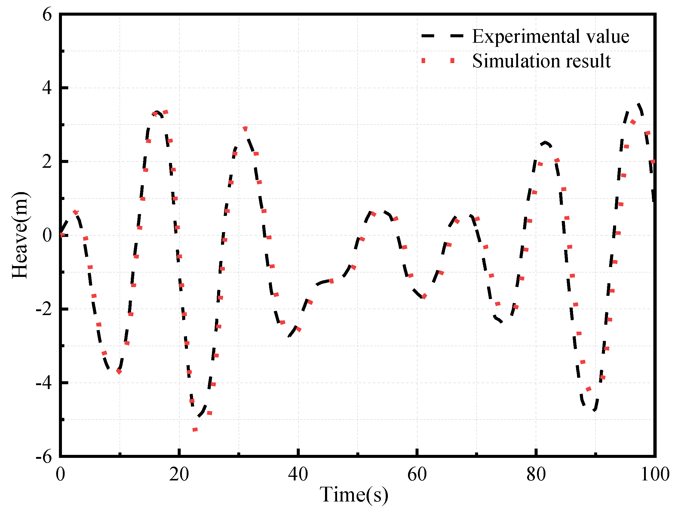
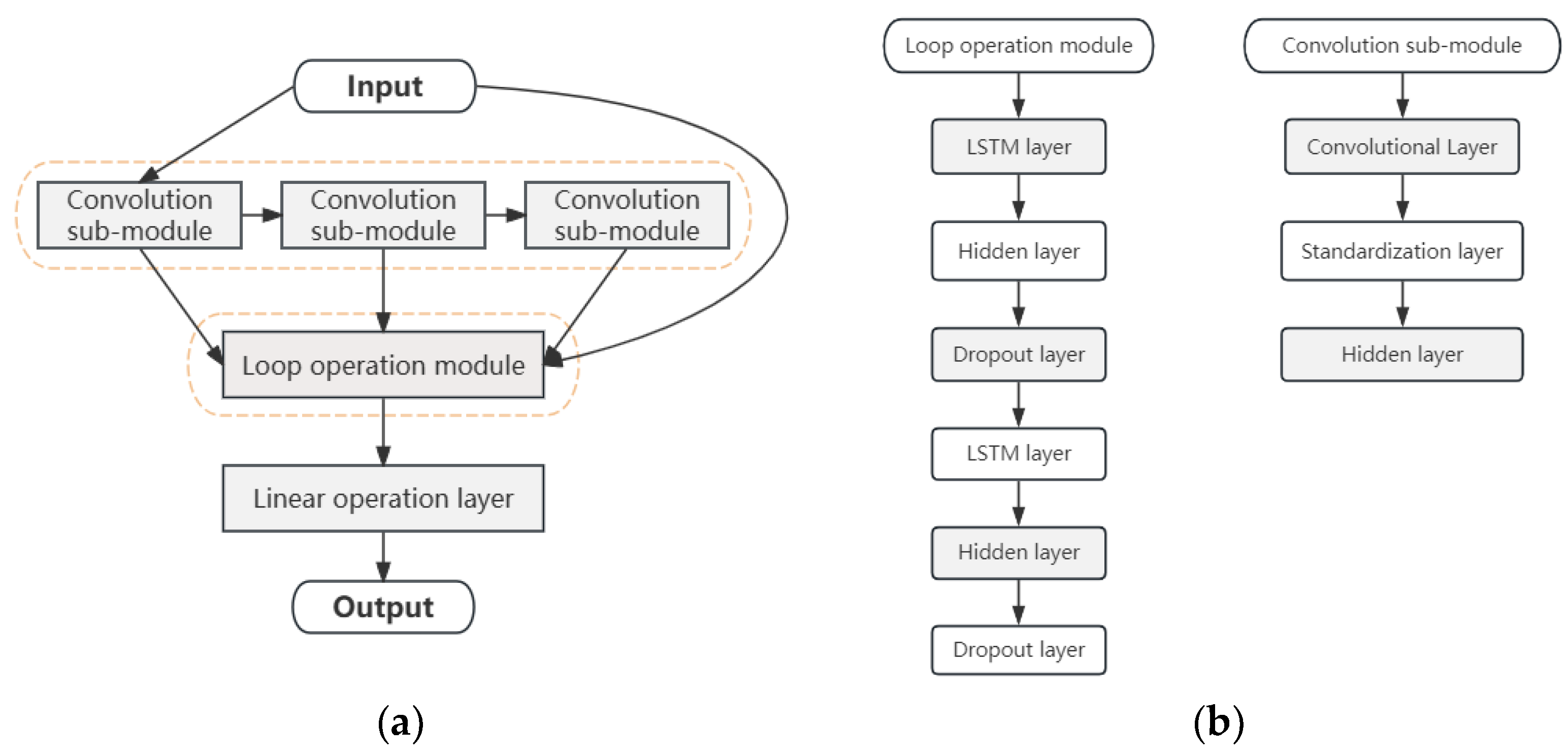
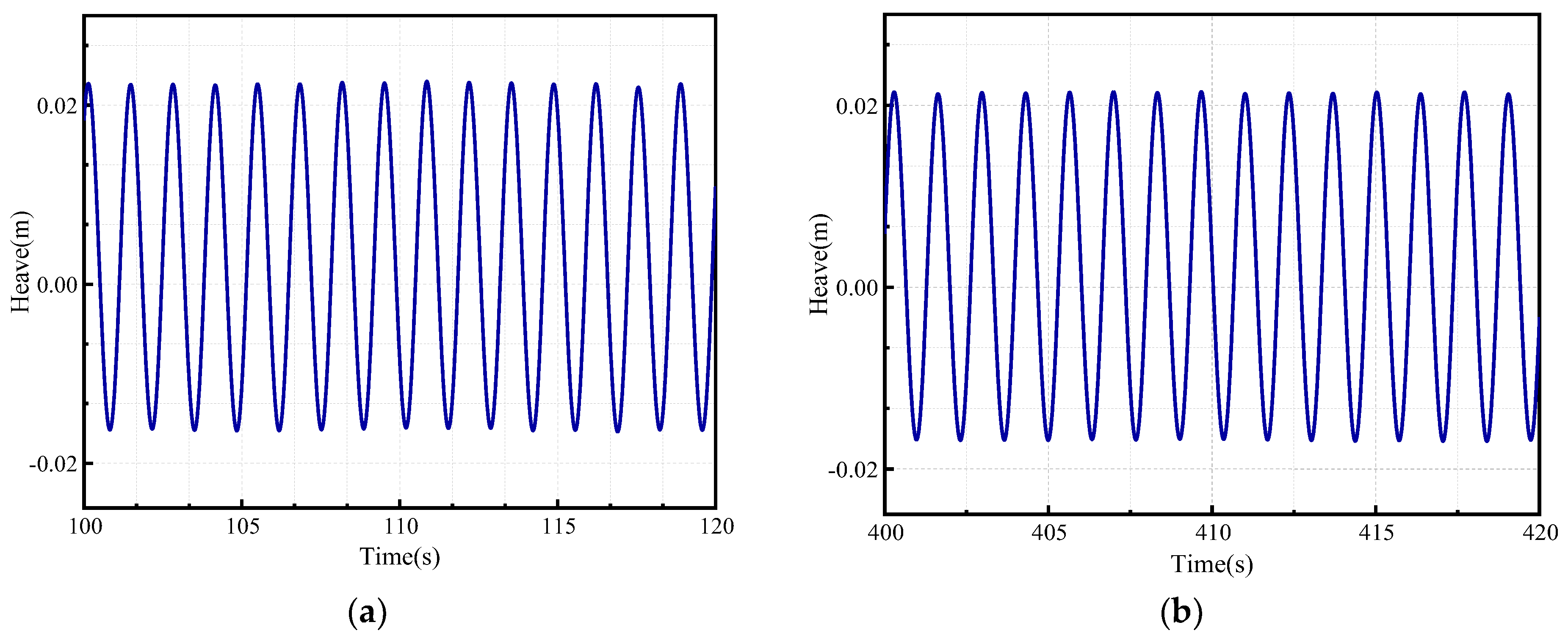
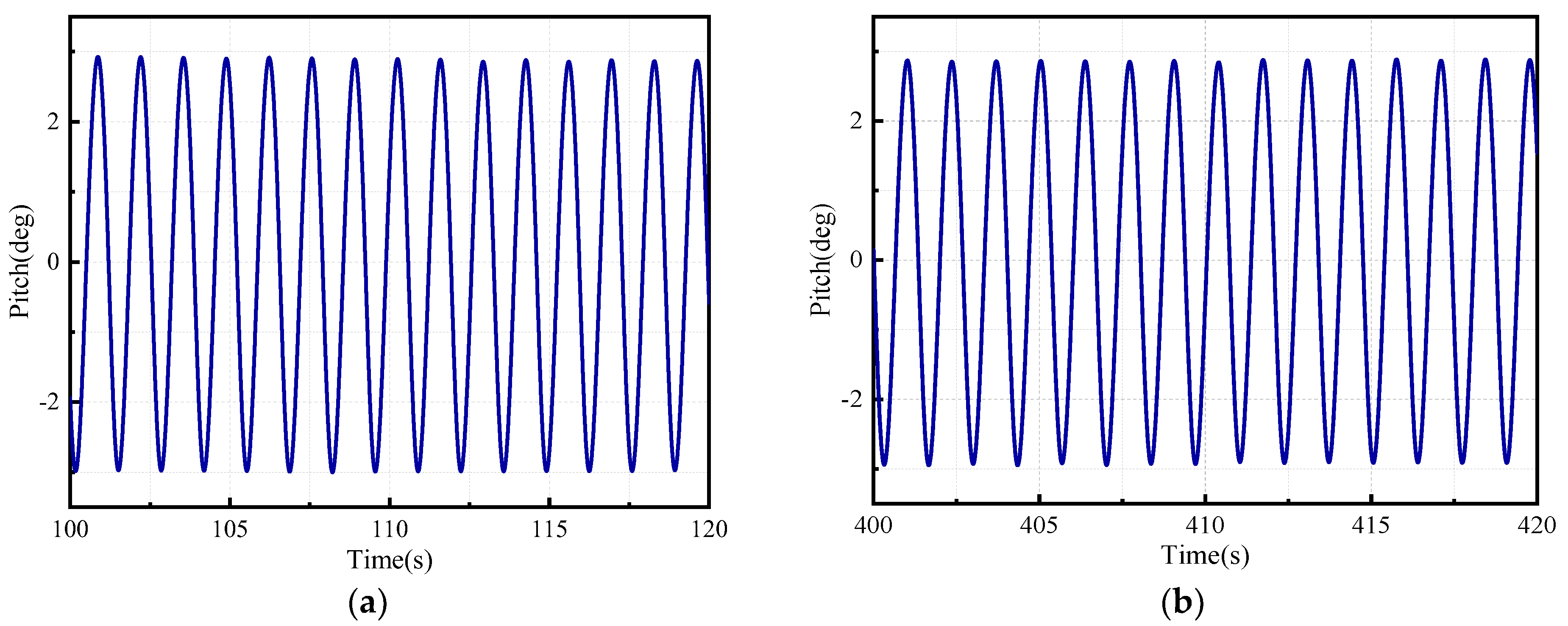
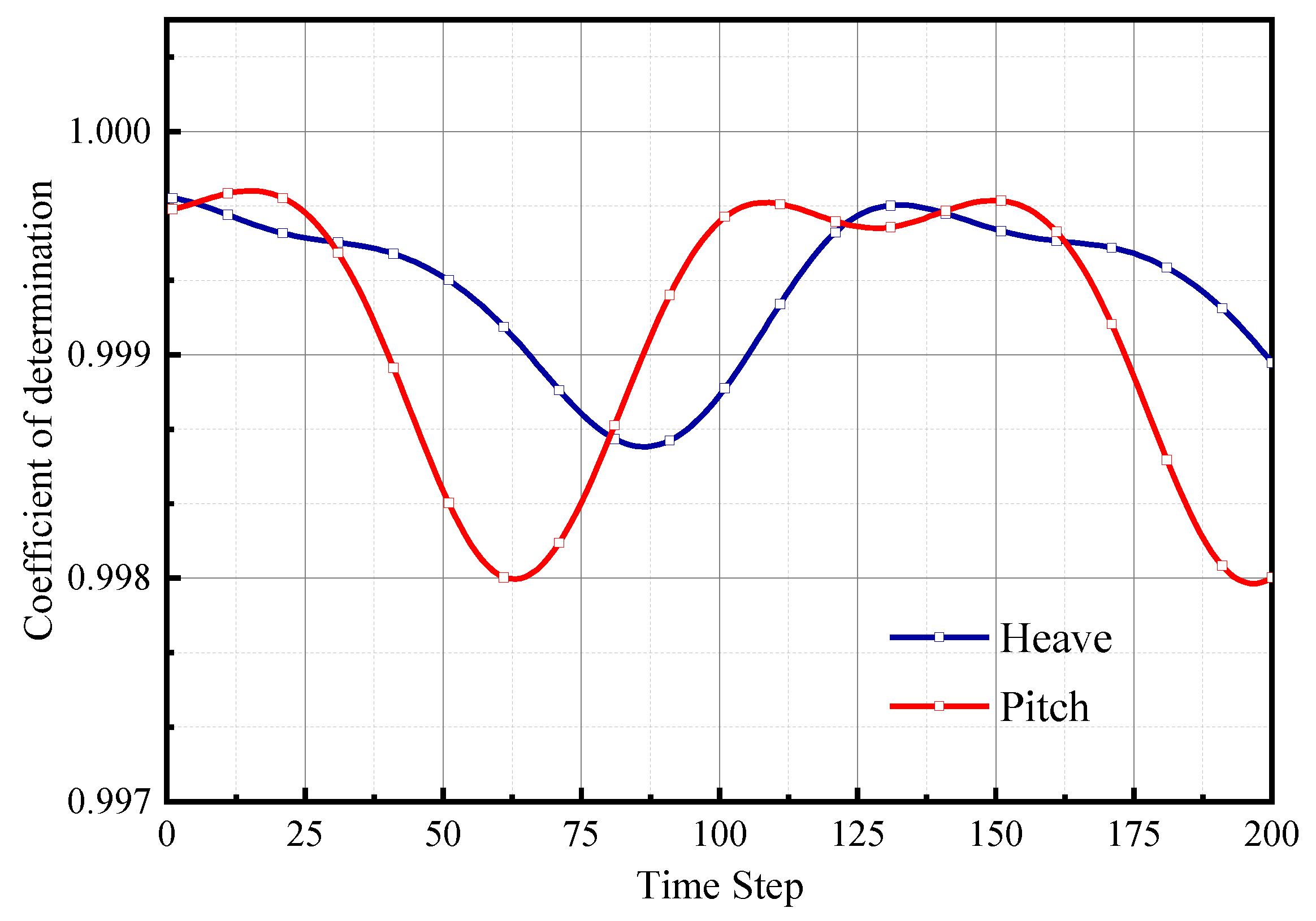
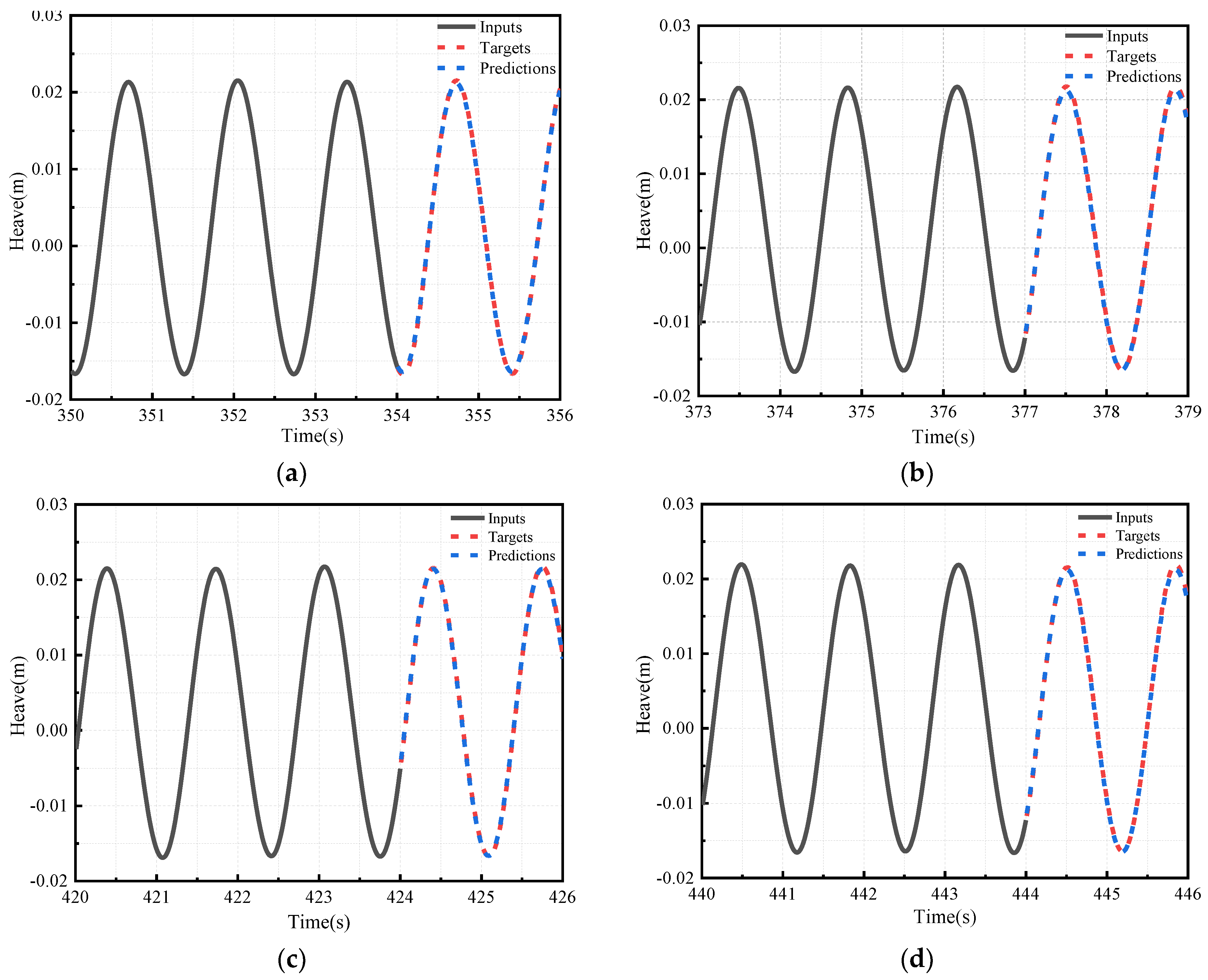
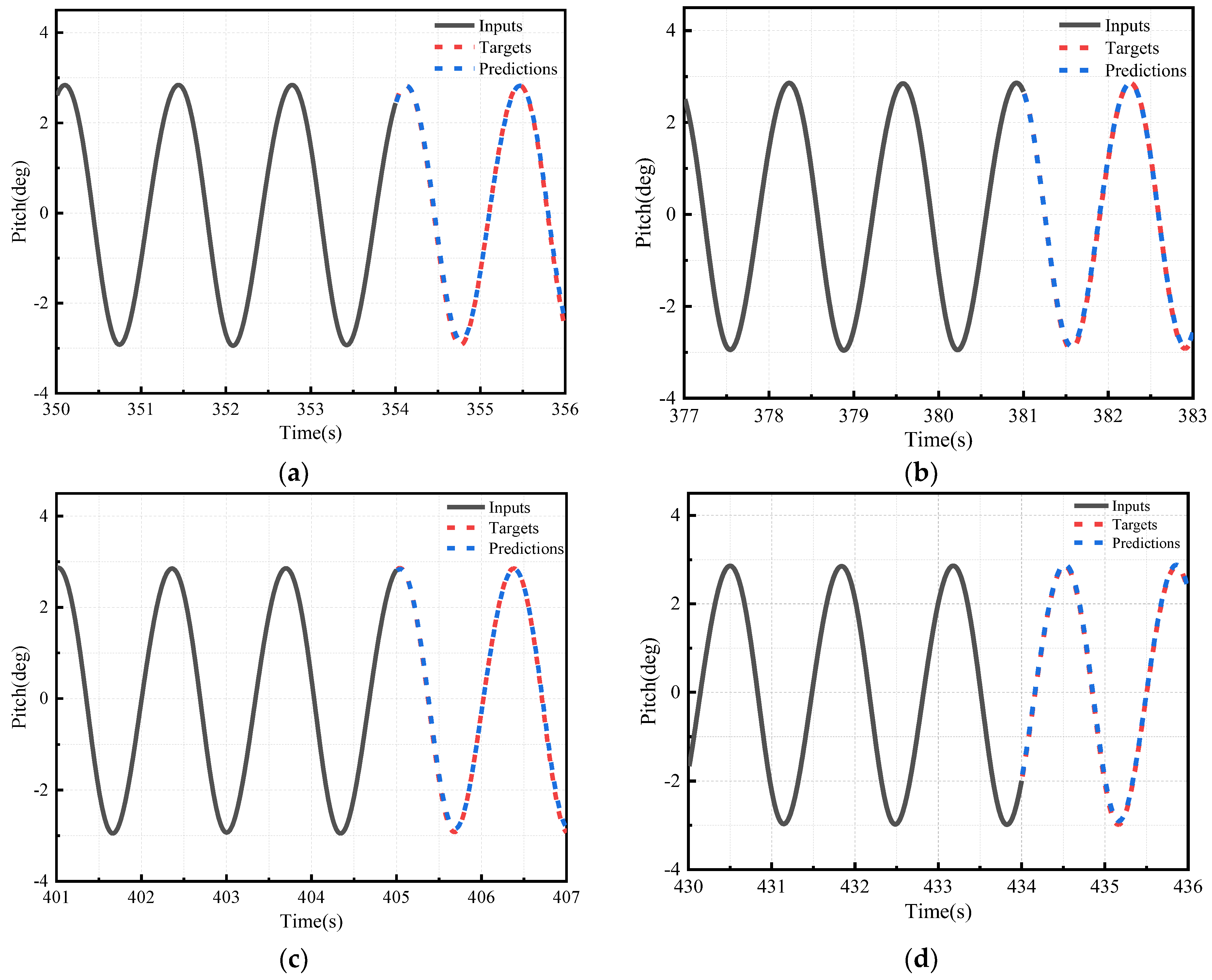
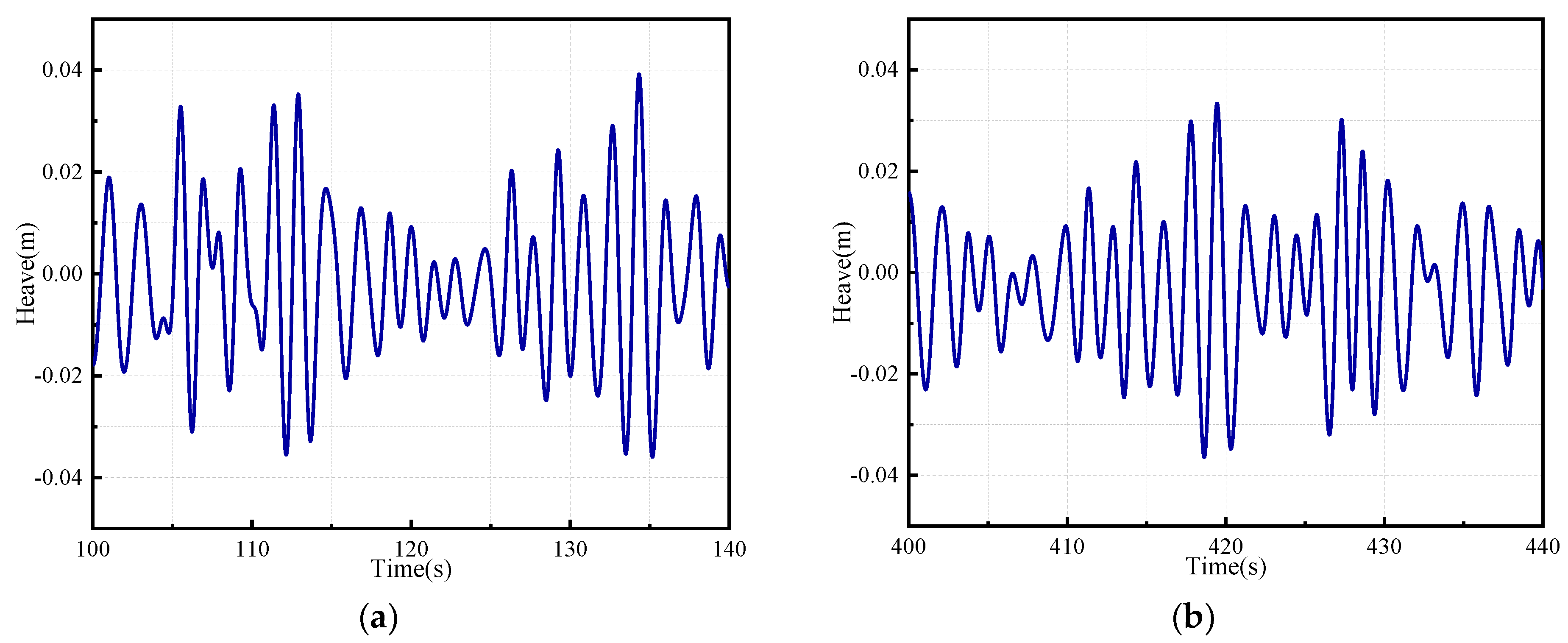
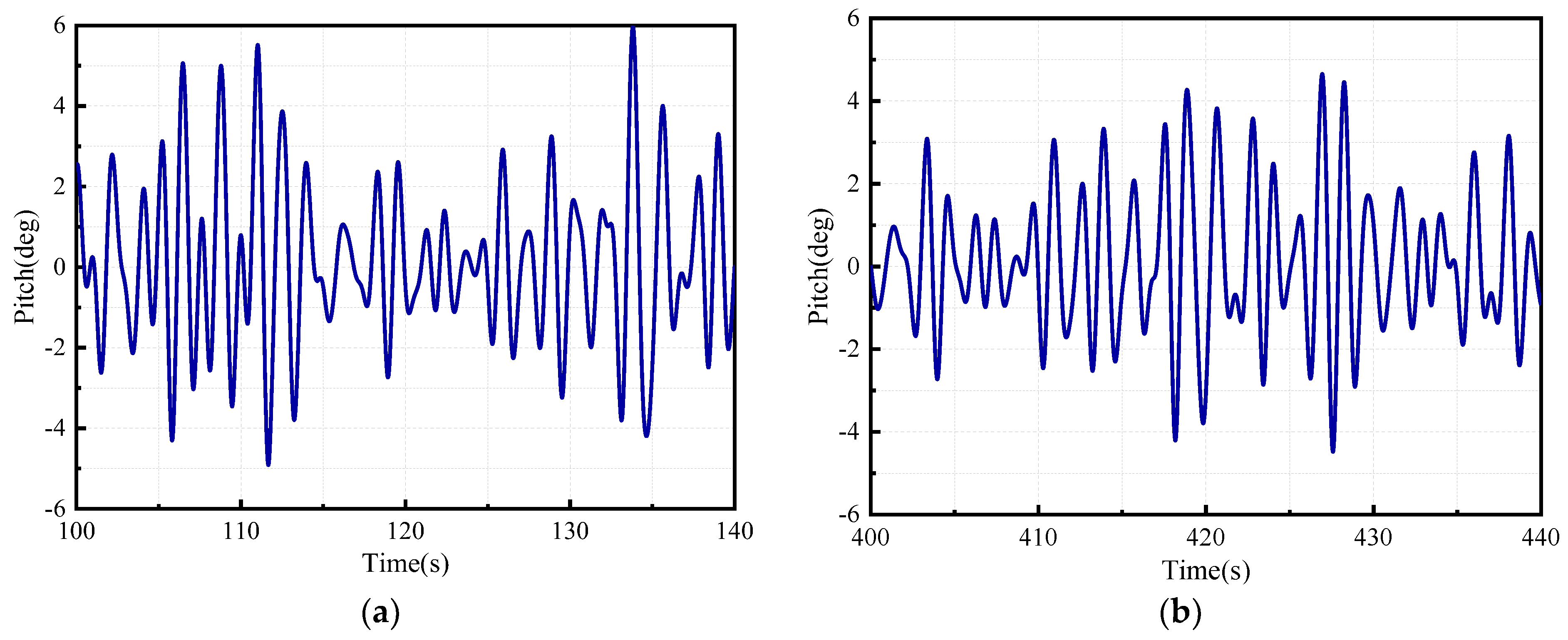
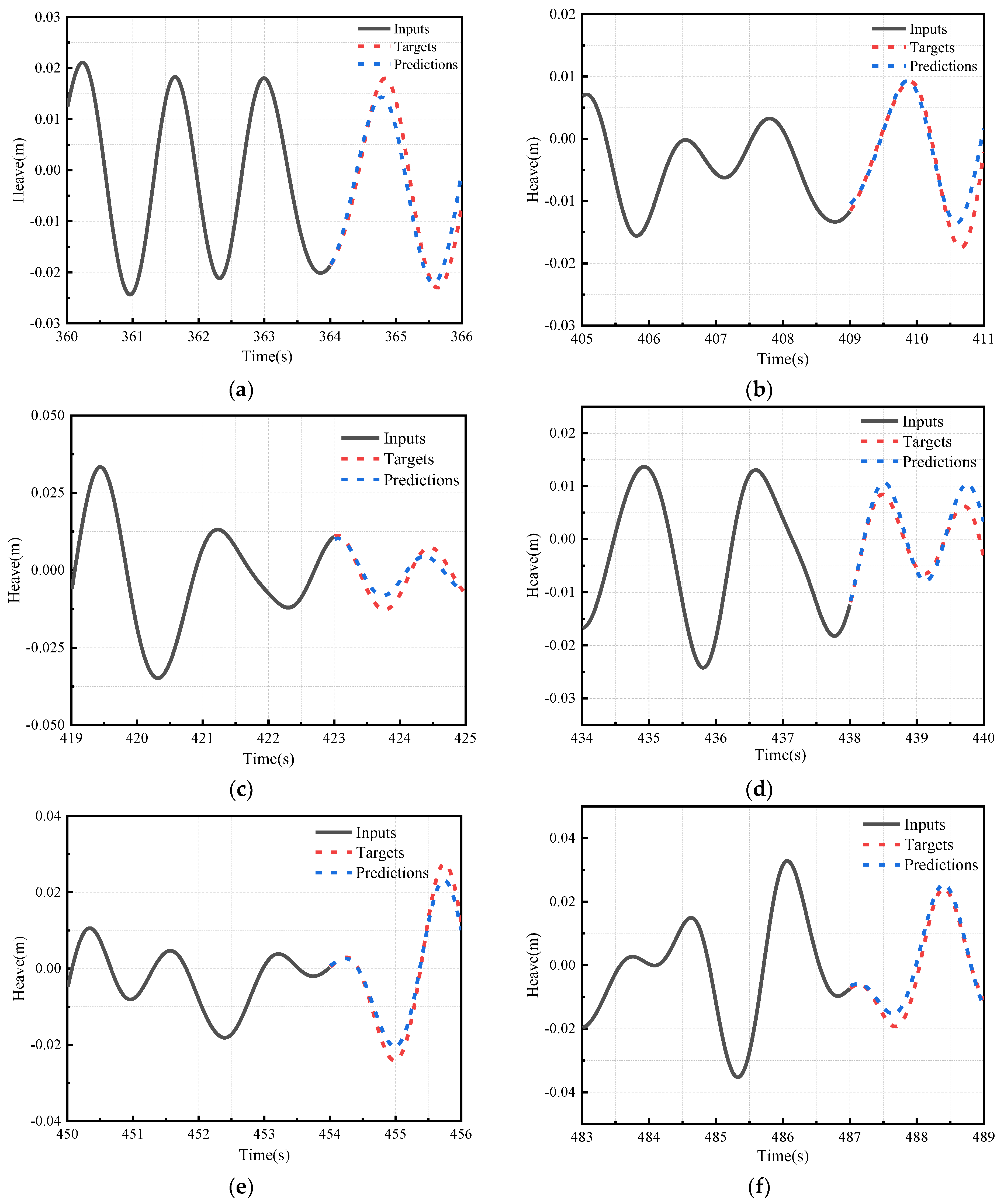
The study of offshore platform motion prediction using neural networks aims to accurately forecast the motion state of offshore platforms in the near future. This is achieved by analyzing large amounts of historical data and leveraging the deep learning capabilities of neural network models. Neural networks are capable of recognizing and processing complex nonlinear relationships within historical data, as well as the combined effects of various environmental factors, demonstrating strong adaptability and learning capabilities. This approach helps in the timely identification of potential risks, prevention of accidents, reduction of operational risks, and provides solid technical support for the sustainable development of ship transportation and offshore engineering. In this study, we first employed the STAR-CCM+2022.1 software to conduct numerical simulations of existing physical experimental data, thereby validating the accuracy of the numerical simulation method. Subsequently, the dynamic responses of offshore platforms under the influence of regular and irregular wave conditions were simulated. To enhance the predictive accuracy, an innovative hybrid forecasting model was proposed, integrating Residual Convolutional Neural Networks (RCNN) with Long Short-Term Memory (LSTM) networks. This model leverages deep learning algorithms to significantly augment the extraction of pertinent features, thereby refining the precision of predictions. Furthermore, a comprehensive evaluation of the forecasting model’s efficacy was conducted employing a triad of evaluative metrics: the Coefficient of Determination (R²), Mean Squared Error (MSE), and Mean Absolute Percentage Error (MAPE). These metrics facilitated a multidimensional error analysis of the model’s predictive outcomes, ensuring the reliability and validity of the prognostications.

2. Basic Theory

2.1. Principle of Neural Network

2.1.1. The Principle of Long Short-Term Memory Neural Networks

Recurrent Neural Networks (RNNs) are specifically designed for processing time series data. Their characteristic is to perform recursive processing along the time axis of the sequence, with nodes in the network connected in a linear chain-like manner [23]. Long Short-Term Memory (LSTM), a derivative type of RNN, was initially proposed by Hochreiter and Schmidhuber [24] and further optimized by Graves [25] to effectively overcome the gradient vanishing problem encountered during RNN training.

Each LSTM unit has a cell to describe its current state. There are three control gates: the input gate, output gate, and forget gate, which are used to control input, output, and cell state, respectively. When a control gate is open, all information can pass through; when closed, no information is allowed to pass. The equations are as follows [26]:

$$ft=\sigma (W_{xy}{x}_t+W_{hf}{h}_t-1+W_{cf}{c}_t-1+b_f)$$

(1)

$$i_t=\sigma (W_{xi}{x}_t+W_{hi}{h}_t-1+W_{ci}{c}_t-1+b_i)$$

(2)

$$c_t=f_t{c}_t-1+i_t\tanh (W_{xc}{x}_t+W_{hc}{h}_t-1+b_c)$$

(3)

$$ot=\sigma (W_{xo}{x}_t+W_{ho}{h}_t-1+W_{co}{c}_t+b_o)$$

(4)

$$h_t=O_t\tanh (c_t)$$

(5)

In the formula, $f_t$ is the forgetting gate equation; $x_t$ is the acceleration at time $t$; $h_{t-1}$ is the output of the hidden layer in the previous time step; $W$ and $b$ are the weight term and bias term of the unit, respectively; $\sigma$ is the activation function; $c_t$ is the input gate equation to update the cell state; and $o_t$ is the output gate equation, which outputs $h_t$ together with $c_t$.

2.1.2. Convolution Layer Principle

The convolutional layer, also known as the convolution operation layer, used in this study is a one-dimensional convolutional layer designed specifically for processing sequence data. As illustrated in Figure 1, the one-dimensional convolution operation involves the convolution kernel moving along the original sequence. At each position, the elements of the kernel are individually multiplied with the corresponding elements in the sequence and summed up to produce a new element, representing the convolution result at that position. After the kernel traverses the entire sequence, a new sequence is formed, representing the convolution operation result of the kernel with the original sequence. The purpose of the convolution operation is to extract different features from the input [27].

2.2. Performance Evaluation Index

After training a machine learning model, it is necessary to evaluate the model’s predictive performance and make improvements based on the evaluation. The metrics used in this paper to describe the model’s prediction bias are Coefficient of Determination (R²), Mean Square Error (MSE), and Mean Absolute Percentage Error (MAPE).

Coefficient Of Determination measures the extent to which the model’s predicted values explain the variability of the actual observations. It is used to assess the goodness of fit between the predicted results and the actual data, with a higher R² value indicating a better fit, closer to 1. Since R² can be negative, it is not a squared value, and a smaller value indicates a poorer fit of the model. Both MSE and MAPE represent the errors between the model’s predicted values and the true values. MSE can be interpreted as the average of the squares of the absolute errors for all samples, while MAPE can be interpreted as the average of the absolute values of the relative errors for all samples. Both MSE and MAPE values are equal to or greater than 0, with better model performance closer to 0, indicating smaller prediction errors [28].

3. Motion Response Verification of Semi-Submersible Platform

To verify the reliability of the numerical simulation method presented in this paper for subsequent studies on platform motion, simulations were compared with experimental data of the heave motion response of a semi-submersible platform, as conducted by Wei Qiangqiang [29]. The experiment was performed in the deep-water test basin of the State Key Laboratory of Ocean Engineering at SHANGHAI JIAO TONG UNIVERSITY. As shown in Figure 2, the physical test model is a semi-submersible platform, downscaled by a factor of 1:60 for calculations. The parameters of the downscaled platform model are shown in

Table 1. Platform parameters.

Parameter	Unit	Original Model	Scale Model
Draught	m	37.0	0.617
Freeboard	m	22.0	0.367
Molded breadth	m	91.5	1.525
Prop spacing	m	70.5	1.175
Column width	m	21.0	0.350
Column height	m	59.0	0.983
Lower hull height	m	9.0	0.150
Lower hull width	m	21.0	0.350
Lower hull length	m	49.5	0.825
Main deck height	m	70.5	1.175

.

The six-degree-of-freedom motion at the center of gravity of the platform model was measured using a non-contact optical six-degree-of-freedom motion measurement system.

The numerical simulation was used to compare and verify the experimental value with a significant wave height of 0.22 m and a peak spectral period of 1.90 s after scaling down. The dimensions of the numerical wave basin were set to 25 m × 20 m × 10 m, with a water depth of 5 m, and the grid division is shown in Figure 3. The heave motions were compared with the experimental data, as shown in Figure 4.

Upon comparing the experimental values with the numerical simulation results, it can be observed that good agreement has been achieved. The simulation accurately reflects the heave motion characteristics of the semi-submersible platform, demonstrating a good level of fit between the results.

4. Motion Response Prediction of Offshore Platform

4.1. Establishment of Neural Network Model

LSTM is a widely recognized classic and simple model for analyzing and forecasting sequential data, with basic sequence fitting capabilities. However, for data with stronger nonlinearity, its fitting capabilities are limited due to its relatively basic computational power. Convolutional layers are used to extract the “spatial features” of data, fitting the information conveyed by the combination of data as a whole. This helps the model better understand the complexity and non-linear relationships in the data, thereby enhancing the accuracy of predictions. The neural network prediction model in this section increases the number of convolutional layers, which helps to increase the depth of the neural network and thus improve its feature extraction capabilities. Furthermore, a skip-connection form of residual structure is introduced to combine the results of multi-level feature extraction. This structure not only preserves the information of the original data but also prevents the training difficulty caused by gradient vanishing during the training process of neural networks.

By merging these two algorithms, the model’s capacity to learn deep features has been augmented in the spatial dimension, enhancing its ability to recognize complex patterns within the data. In the temporal dimension, the model’s precision in forecasting trends in time series has been elevated. This multidimensional approach effectively captures the intrinsic characteristics of the data, overcoming the limitations of traditional prediction algorithms that struggle to effectively capture features in complex and highly nonlinear datasets. Through the collaborative effect of both spatial and temporal dimensions, this model is capable of more accurately understanding and predicting the dynamics of data changes.

In the following sections, we will refer to this model as ResCNN-LSTM. The computational workflow is illustrated in Figure 5.

4.2. Model Prediction Analysis Under the Action of Regular Waves

4.2.1. Gathering Data and Training Models

The numerical water tank was constructed based on a scaled down model with a scale ratio of 1:50. The specific dimensions are 15 m in length, 8 m in width, and 5.5 m in molding depth. The tank has a depth of 4 m below the waterline. The X-axis direction is defined as the head wave direction, with the incident angle of regular waves set at 0°. The specific operating conditions are illustrated in

Table 2. Parameters of wave.

	Wave Height	Wave Period
Model	0.07 m	1.34 s
Prototype (before scale)	3.5 m	9.5 s

. In this section, the use of a mooring system is not considered, focusing on the analysis of heave and pitch motion modes, thereby constraining sway, surge, yaw, and roll motion modes.

Table 3. The working condition parameters of the original model and the scale model of the platform [30].

Parameter	Platform Original Model	Scale Model
Drainage volume	5.53 × 106 kg	44.21 kg
Draught	6.897 m	0.1379 m
Height of center of gravity	6.615 m	0.1323 m
Roll moment of inertia	1.08 × 109 kg·m2	3.46 kg·m2
Pitching moment of inertia	1.19 × 109 kg·m2	3.81 kg·m2
Bow moment of inertia	1.56 kg·m2	5.01 kg·m2

presents the model condition parameters.

The computational model employed a turbulence model, utilizing an implicit unsteady time solver with second-order temporal discretization. The left boundary was designated as a velocity inlet, the top and right boundaries were set as pressure outlets, the bottom was modeled as a wall, and the front and back were established as symmetric planes. A damping zone was introduced at the right outlet using the VOF wave option to minimize wave reflection. Figure 6 depicts the numerical computational domain.

To ensure the accuracy of the numerical simulation results, the computational domain underwent grid refinement treatment, with layer-by-layer refinement to increase grid precision and computational accuracy, as shown in Figure 7. Figure 8 and Figure 9 depict the time history curves of heave and pitch motion modes, respectively.

From the figures, it can be observed that under the action of regular waves, there is a distinct interaction between the platform and the waves. The heave and pitch motions exhibit a certain correlation with the wave frequency, consequently showing clear regularity in their time history curves. This regularity results in relatively smooth envelopes of the time history curves for heave and pitch motions.

The dataset was split into training and testing sets based on chronological order using a 70–30% ratio. With a time step of 0.01 s in the numerical simulation, the training sets for heave and pitch consist of 35,000 time steps each, while the testing sets consist of 15,000 time steps each. The prediction strategy involves multi-step forecasting, using four seconds of motion data as input to predict the subsequent two seconds of motion data. After fine-tuning, the model’s specific parameter configuration is presented in

Table 4. Relevant parameter settings of the algorithm.

Parameter	Value
TensorFlow random number seed	2023
The number and size of convolution layer kernels	2, 4
The kernel size of the LSTM layer	256, 128
Hidden layer activation function	Hyperbolic tangent function
Optimizer for training models	Adam
Initial training learning rate	0.001
The number of training iteration cycles	100

.

4.2.2. Display and Analysis of Prediction Results

Following the model training, an analysis of the prediction results was conducted. First, examining the R² metric, the computation results of ResCNN-LSTM on the heave and pitch testing sets are illustrated in Figure 10.

From the figure, it can be observed that there are no time steps in the model predictions for heave and pitch motions that cannot be fitted. This indicates that the ResCNN-LSTM model can effectively capture and reflect the characteristics of heave and pitch motions under regular waves, without any significant prediction deviations or fitting failures. As indicated in Section 2.2, the closer the R² value is to 1, the stronger the model’s fitting ability to the data. In the graph, the R² values for each time step of heave and pitch motions are all greater than 0.9, indicating that the ResCNN-LSTM model demonstrates outstanding capabilities in predicting heave and pitch motions under regular wave conditions. This implies the model’s good capture of complex patterns and dynamic variations in the data.

MSE calculates the average of the squared differences between the predicted values and the actual values of the samples, used to evaluate the accuracy of the model’s predictions for the heave and pitch data sequences. The MSE value ranges from zero to positive values, where values closer to zero indicate smaller prediction deviations. MAPE calculates the average of the absolute percentage errors of all samples. In comparison to MSE, MAPE focuses more on the overall situation. It ranges from 0 onwards, with values closer to 0 indicating smaller prediction errors. From

Table 5. MSE and MAPE values.

Evaluation Index	Heave	Pitch
MSE	1.24 × 10−7	3.64 × 10−7
MAPE	0.15	0.16

, it can be observed that for both heave and pitch, the MSE and MAPE values are very close to 0. This indicates that the model has good predictive capabilities for the heave and pitch data sequences, with small prediction errors. Such results further confirm the accuracy of the R² values, indicating a high level of model fitting to the data.

In general, the motion response data sequences generated under regular waves exhibit clear periodicity and regularity, without complex dynamic behaviors. The model can leverage the regularity information present in historical data to infer future motion states, making the predictions relatively easy and highly accurate. To provide a qualitative analysis of the predictive performance of the ResCNN-LSTM model, four individual samples from the heave and pitch testing sets were selected to showcase the prediction results, as shown in Figure 11 and Figure 12.

From Figure 11 and Figure 12, it can be observed that the ResCNN-LSTM model demonstrates good fitting performance on the testing sets for both pitch and heave motions. It successfully captures the patterns and relationships between the data, showing no significant deviations in predicting peak and trough values, thus exhibiting a high degree of forecasting accuracy. These results further validate the accuracy of the three evaluation metrics mentioned above.

4.3. Model Prediction Analysis Under Irregular Waves

4.3.1. Data Acquisition and Model Training

The motion response data of offshore platforms under irregular waves exhibit complex nonlinear characteristics. This nonlinearity is reflected in the irregular fluctuations seen in the time history curves of the motion response data. The numerical wave tank model is constructed based on a scaled-down representation, with dimensions set at a length of 15 m, width of 8m, model depth of 5.5 m, and an additional depth of 4 m below the waterline. Moreover, there is an 8 m-long wave dissipation zone. The irregular waves approach at an angle of 0°, with the X-axis direction being the head sea direction. The specific operating conditions are detailed in

Table 6. Parameters of wave.

	Significant Wave Height	Spectrum Peak Period	Number of Wave Components
Model	0.07 m	1.41 s	75
Prototype (before scale)	3.5 m	10 s	75

. Figure 13 depicts the numerical computational domain.

This numerical simulation modeled the heave and pitch motions of a four-column offshore platform under irregular waves with a wave approach angle of 0 degrees. The specific time history curves of the motions are illustrated in Figure 14 and Figure 15.

From the figures, it can be seen that the heave and pitch motions exhibit a certain correlation trend with the frequency of the waves, resulting in a striking resemblance between the time history curves of heave and pitch motions and the significant wave height time history curves. During the dataset generation process, the data was split into training and testing sets in a 70% to 30% ratio, following chronological order. With a numerical simulation time step of 0.01s, the training sets for heave and pitch consist of 35,000 time steps each, while the testing sets consist of 15,000 time steps each. The prediction strategy involves using a multi-step forecasting method, taking four seconds of motion data as input to predict the subsequent two seconds of motion data by analyzing and learning patterns and trends in the historical data. Compared to single-step prediction, using a longer time window allows the model to forecast a longer time window as well. After tuning, the specific parameter configuration of the model is provided in

Table 7. Relevant parameter settings of the algorithm.

Parameter	Value
TensorFlow random number seed	2023
The number and size of convolution layer kernels	2, 4
The kernel size of the LSTM layer	512, 256
Hidden layer activation function	Hyperbolic tangent function
Optimizer for training models	Adam
Initial training learning rate	0.001
The number of training iteration cycles	150

.

4.3.2. Prediction Results and Analysis

After training the model as described above, an analysis of the forecasting results was conducted. Firstly, looking at the R² metric, the calculated results for the heave and pitch testing sets of the ResCNN-LSTM model are shown in Figure 16.

The figure demonstrates that the model successfully fits both heave and pitch motions across the entire predicted time range, with no instances of failed fitting. For the heave motion, R² values consistently exceed 0.6 throughout the predicted time range, indicating that the ResCNN-LSTM model effectively captures the characteristics of heave motion under irregular wave conditions. Even when faced with strong nonlinearity in the time history curves, the model exhibits good fitting capabilities, resulting in balanced and effective predictions overall. Regarding pitch motion, the model’s overall R² values are slightly lower compared to those for heave motion. This can be attributed primarily to the offshore platform’s four-column structure, which leads to significant fluid-resonance issues under these conditions. Consequently, the pitch motion exhibits stronger nonlinearity, presenting a greater challenge for prediction. Nevertheless, R² values remain above 0.2 throughout the entire predicted time range, demonstrating that the ResCNN-LSTM model effectively captures variations in pitch motion data. This indicates the model’s ability to dynamically respond to changes in the data without experiencing fitting failures.

Both MSE (Mean Squared Error) and MAPE (Mean Absolute Percentage Error) metrics perform better as their values approach zero.

Table 8. MSE and MAPE values.

Evaluation Index	Heave	Pitch
MSE	1.91 × 10−3	8.59 × 10−3
MAPE	0.55	0.58

shows that for both heave and pitch motions, the MSE and MAPE values are very close to zero. This indicates minimal differences between predicted and actual values, as well as low relative errors in the predictions. These results signify that the model demonstrates good fitting capabilities for both heave and pitch motion data sequences within the predicted time range. Furthermore, these findings corroborate the accuracy of the R² values as an evaluation metric.

Overall, the interaction between offshore platforms and irregular waves results in motion responses with strong nonlinearity. The time-series data exhibits complex dynamical behaviors, yet the ResCNN-LSTM model can still make accurate predictions. This is mainly attributed to the model’s ability to extract spatial features from the input data through convolutional layers and capture temporal information using long short-term memory networks. This combination enables the model to better handle complex nonlinear relationships and temporal dependencies. For a qualitative analysis of the model’s prediction performance, six individual samples from the heave and pitch testing sets were selected to demonstrate the prediction results, as shown in Figure 17 and Figure 18.

Figure 17 and Figure 18 clearly demonstrate the ResCNN-LSTM model’s outstanding fitting performance on the testing sets for both pitch and heave motions. The model successfully captures the distribution patterns and relationships within the data, particularly in regions where the curves exhibit rapid changes. Through inductive fitting, the model deduces highly accurate predictions. Moreover, the ResCNN-LSTM model exhibits high accuracy in predicting both the rising and falling trends of the curves. It precisely predicts the peak and trough values, displaying a very high level of prediction precision. These intuitive prediction sample graphs indirectly validate the accuracy of the three evaluation metrics: R², MSE, and MAPE.

5. Conclusions

After conducting predictive analysis on the motion responses of offshore platforms under both regular and irregular wave conditions, the results reveal that despite the significant nonlinearity of platform motions, the ResCNN-LSTM model accurately identifies their motion characteristics and effectively predicts their subsequent states. This demonstrates the model’s ability to achieve precise predictions for the heave and pitch motions of offshore platforms. The model’s outstanding performance across the three key evaluation metrics validates its exceptional adaptability and sensitivity in capturing data correlations. This finding confirms the effectiveness of the ResCNN-LSTM model in predicting offshore platform motion responses, which has profound implications for advancing the field of ocean engineering. Nonetheless, the model’s predictive accuracy over extended timeframes requires further empirical validation. However, there is no doubt that the ResCNN-LSTM model, while handling complex and nonlinear motion patterns, maintains high predictive accuracy, demonstrating its potential as a valuable tool for improving the safety and efficiency of offshore operations. Through accurate forecasting, it is possible to optimize the operational strategies of offshore platforms, reduce unnecessary fuel consumption, and thus achieve the dual goals of cost savings and environmental benefits. At the same time, accurate prediction of motion responses can identify potential safety risks in advance, take preventive measures, and effectively enhance the safety of operations. Moreover, the model’s rapid adaptation to various situations during the operation process significantly enhances the operational efficiency of offshore platforms.

Therefore, with the continuous advancement of technology and the deepening of applications, ResCNN-LSTM model is expected to become an important tool to promote the development of the ocean engineering field towards higher reliability, stronger safety, better economy, and better environmental protection. Future research can further explore the stability of the model over a longer period and its applicability under different oceanic environmental conditions, in order to achieve broader practical applications.

References

1. Cheng, X.; Li, G.; Skulstad, R.; Major, P.; Chen, S.; Hildre, H.P.; Zhang, H. Data-driven uncertainty and sensitivity analysis for ship motion modeling in offshore operations. Ocean Eng. 2019, 179, 261–272. [Google Scholar]
2. Kang, Y.; Chen, P.; Cheng, Z.; Hu, Z. Overview of the application of artificial intelligence technology in the field of offshore wind turbines. Ship 2023, 34, 12–23. [Google Scholar]
3. Xie, Y.; Zhou, S.; Wang, F. Prediction Analysis of Sea Level Change in the China Adjacent Seas Based on Singular Spectrum Analysis and Long Short-Term Memory Network. J. Mar. Sci. Eng. 2024, 12, 1397. [Google Scholar] [CrossRef]
4. Qin, T.; Chen, R.; Qin, R.; Yu, Y. Improved Hierarchical Temporal Memory for Online Prediction of Ocean Time Series Data. J. Mar. Sci. Eng. 2024, 12, 574. [Google Scholar] [CrossRef]
5. Ouyang, Z.; Gao, Y.; Zhang, X.; Wu, X.; Zhang, D. Significant Wave Height Forecasting Based on EMD-TimesNet Networks. J. Mar. Sci. Eng. 2024, 12, 536. [Google Scholar] [CrossRef]
6. Hou, X.; Xia, S. Short-Term Prediction of Ship Roll Motion in Waves Based on Convolutional Neural Network. J. Mar. Sci. Eng. 2024, 12, 102. [Google Scholar] [CrossRef]
7. Martić, I.; Degiuli, N.; Grlj, C.G. Prediction of Added Resistance of Container Ships in Regular Head Waves Using an Artificial Neural Network. J. Mar. Sci. Eng. 2023, 11, 1293. [Google Scholar] [CrossRef]
8. Elkhrachy, I.; Alhamami, A.; Alyami, S.H.; Alviz-Meza, A. Novel Ocean Wave Height and Energy Spectrum Forecasting Approaches: An Application of Semi-Analytical and Machine Learning Models. Water 2023, 15, 3254. [Google Scholar] [CrossRef]
9. Hu, L.; Zhang, M.; Yuan, Z.-M.; Zheng, H.; Lv, W. Predictive Control of a Heaving Compensation System Based on Machine Learning Prediction Algorithm. J. Mar. Sci. Eng. 2023, 11, 821. [Google Scholar] [CrossRef]
10. Gu, D.; Shi, Z.; Chen, G.; Wang, H. A Prediction Method for Ship Motion Pose Based on Neural Networks. J. Ship Sci. Technol. 2022, 44, 55–59. [Google Scholar]
11. Gao, N.; Chuang, Z.; Hu, A. Real-time prediction of ship motion based on improved empirical mode composition and dynamic residual neural network. Ocean. Eng. 2024, 292, 116528. [Google Scholar] [CrossRef]
12. Tian, X.; Song, Y. Machine Learning for Short-Term Prediction of Ship Motion Combined with Wave Input. Appl. Sci. 2023, 13, 5298. [Google Scholar] [CrossRef]
13. Gao, M.; Shi, G.; Li, S. Online Prediction of Ship Behavior with Automatic Identification System Sensor Data Using Bidirectional Long Short-Term Memory Recurrent Neural Network. Sensors 2018, 18, 4211. [Google Scholar] [CrossRef] [PubMed]
14. Wang, K.; Li, G. DRNN Neural Network for Time Series Prediction of Ship Roll Motion. J. Harbin Eng. Univ. 1997, 18, 41–47. [Google Scholar]
15. Xu, P.; Jin, H.; Wang, K.; Yan, L. A Novel Real-Time Prediction Method for Ship Roll Motion. China Shipbuild. 2002, 43, 72–76. [Google Scholar]
16. Xie, M.; Zhao, X. Short term prediction of large ship motion based on projection pursuit learning. Ship Mech. 2000, 4, 28–32. [Google Scholar]
17. Khan, A.; Bil, C.; Marion, K.E. Ship motion prediction for launch and recovery of air vehicles. In Proceedings of the OCEANS 2005 MTS/IEEE, Washington, DC, USA, 18–23 September 2005; IEEE: Piscataway, NJ, USA, 2005; pp. 2795–2801. [Google Scholar]
18. Khan, A.; Marion, K.; Bil, C. Refereed The Prediction of Ship Motions and Attitudes Using Artificial Neural Networks. ASOR Bull. 2008, 26, 2–6. [Google Scholar]
19. Li, H.; Xiao, L.; Wei, H.; Liu, M. Research on Online Prediction of Motion of Floating Offshore Platforms Based on LSTM Network. Ship Mech. 2021, 25, 576–585. [Google Scholar]
20. Wu, Y.; Wei, N.; Liu, F. Application of Wavelet Multi-Scale Time Series in Ultra-Short-Term Prediction of Ship and Offshore Platform Motion. Ship Ocean Eng. 2012, 41, 147–150. [Google Scholar]
21. Hou, J.; Dong, F.; Cai, F. Ultra-Short-Term Prediction of Ship Oscillatory Motion Combining Chaos Theory and Neural Networks. J. Ship Sci. Technol. 2008, 1, 67–70. [Google Scholar]
22. Biswas, S.; Panigrahi, B.K.; Nayak, P.K.; Pradhan, G.; Padmanaban, S. A Single-Pole Filter-Assisted Improved Protection Scheme for the TCSC-Compensated Transmission Line Connecting Large-Scale Wind Farms. IEEE J. Emerg. Sel. Top. Ind. Electron. 2024, 5, 346–358. [Google Scholar] [CrossRef]
23. Goodfellow, I.; Bengio, Y.; Courville, A. Deep Learning; MIT Press: Cambridge, MA, USA, 2016. [Google Scholar]
24. Hochreiter, S.; Schmidhuber, J. Long short-term memory. Neural Comput. 1997, 9, 1735–1780. [Google Scholar] [CrossRef] [PubMed]
25. Graves, A. Supervised Sequence Labelling with Recurrent Neural Networks. Ph.D. Thesis, Technical University of Munich, Munich, Germany, 2008. [Google Scholar]
26. Wei, Q. Analysis and Prediction of Motion Response of Semi-Submersible Platform Based on Deep Learning. Master’s Thesis, Shanghai Jiao Tong University, Shanghai, China, 2021. [Google Scholar] [CrossRef]
27. Zhang, S. Research on Neural Network-Based Algorithm for Instantaneous Wave Height Prediction. Master’s Thesis, Jiangsu University of Science and Technology, Zhenjiang, China, 2024. [Google Scholar]
28. Yang, J. Research on Dynamic Tension Prediction Method of Single-Point Mooring System Based on Deep Learning. Master’s Thesis, Harbin Engineering University, Harbin, China, 2022. [Google Scholar] [CrossRef]
29. Wei, Q.; Li, X.; Li, X.; Lu, W. Ultra-Short-Term Forecasting of Semi-Submersible Platform Motion Based on EMD-LSTM Model. Ocean Eng. 2021, 39, 29–37. [Google Scholar] [CrossRef]
30. Niu, G. Influence of Float Shape on the Motion Performance of Offshore Satellite Launch Platforms. Master’s Thesis, Jiangsu University of Science and Technology, Zhenjiang, China, 2021. [Google Scholar] [CrossRef]
Figure 1. Diagram of one-dimensional convolution operation.
Jmse 12 01869 g001
Figure 2. Semi-submersible platform model.
Jmse 12 01869 g002
Figure 3. Grid division situation. (a) Y-axis direction. (b) Z-axis direction.
Jmse 12 01869 g003
Figure 4. The comparison of heave motion between experimental value and simulation result.
Jmse 12 01869 g004
Figure 5. Computational flow graph of ResCNN-LSTM. (a) ResCNN-LSTM flowchart. (b) Submodule flowchart.
Jmse 12 01869 g005
Figure 6. Numerical computation field. (a) Partial view from Y-axis perspective. (b) Overall view from Z-axis perspective.
Jmse 12 01869 g006
Figure 7. Mesh subdivision. (a) Z-axis direction. (b) Y-axis direction.
Jmse 12 01869 g007
Figure 8. The time-history curve of heave motion. (a) 100–120 s local diagram, (b) 400–420 s local diagram.
Jmse 12 01869 g008
Figure 9. The time-history curve of pitch motion. (a) 100–120 s local diagram, (b) 400–420 s local diagram.
Jmse 12 01869 g009
Figure 10. R2 comparison diagram.
Jmse 12 01869 g010
Figure 11. Heave test set single sample prediction result diagram. (a) 350–356s. (b) 373–379s (c) 420–426s (d) 440–446s.
Jmse 12 01869 g011
Figure 12. Pitch test set single sample prediction result diagram. (a)350–356s. (b) 377–383s (c) 401–407s (d) 430–436s.
Jmse 12 01869 g012
Figure 13. Numerical computation field. (a) Partial view from Y-axis perspective. (b) Overall view from Z-axis perspective.
Jmse 12 01869 g013
Figure 14. The time-history curve of heave motion. (a) 100–140 s local diagram, (b) 400–440 s local diagram.
Jmse 12 01869 g014
Figure 15. The time-history curve of pitch motion. (a) 100–140 s local diagram, (b) 400–440 s local diagram.
Jmse 12 01869 g015
Figure 16. R2 comparison diagram.
Jmse 12 01869 g016
Figure 17. Heave test set single sample prediction result diagram. (a) 360–366 s. (b) 405–411 s (c) 419–425 s (d) 434–440 s (e) 450–456 s (f) 483–489 s.
Jmse 12 01869 g017
Figure 18. Pitch test set single sample prediction result diagram. (a) 357–363 s. (b) 390–396 s (c) 415–421 s (d) 445–451 s. (e) 458–464 s (f) 485–491 s.
Jmse 12 01869 g018