
Salmon Salar Optimization: A Novel Natural Inspired Metaheuristic Method for Deep-Sea Probe Design for Unconventional Subsea Oil Wells


Abstract
1. Introduction
2. Related Works
3. Materials and Methods
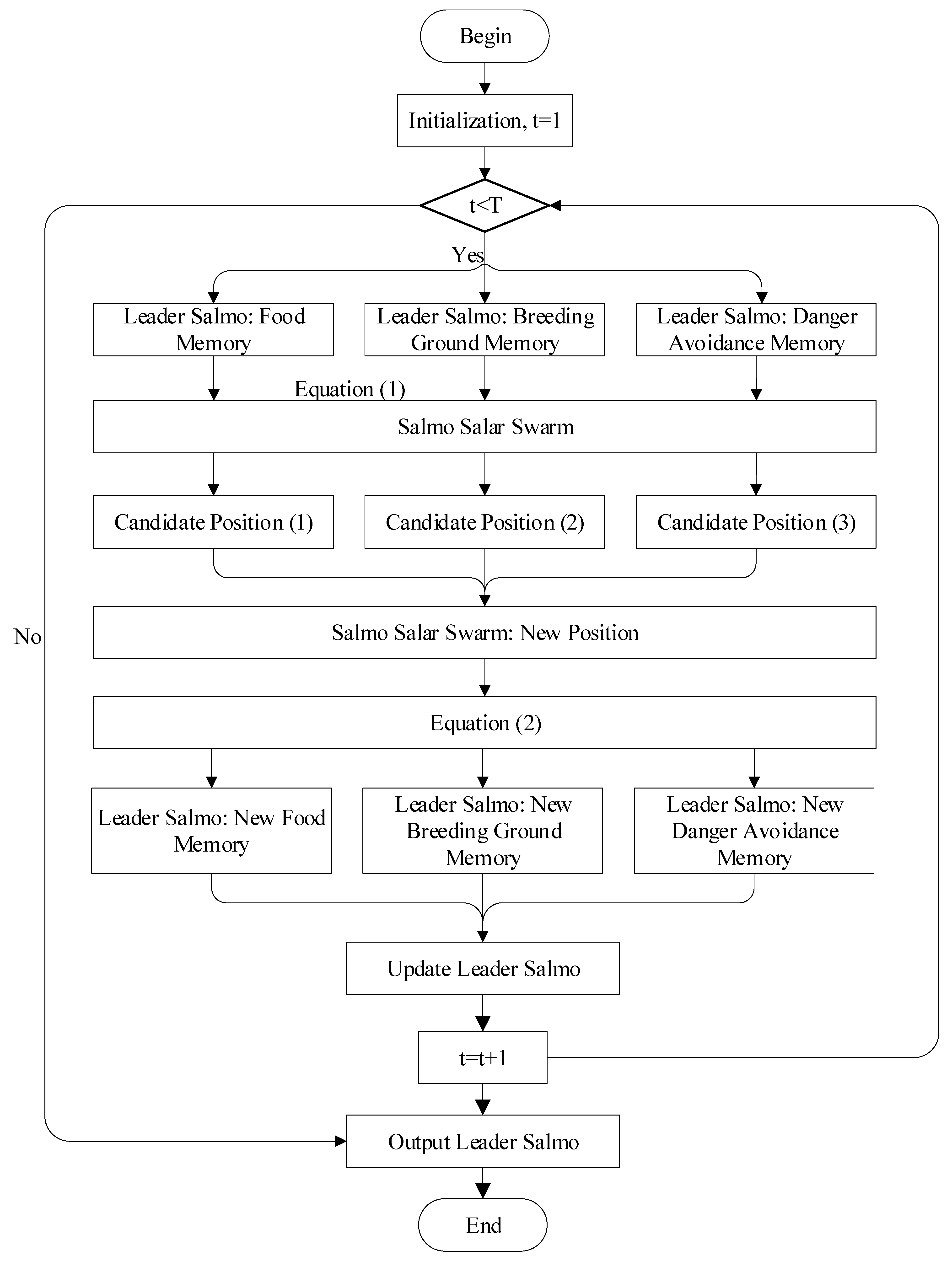
3.1. Salmon Salar Optimization
3.2. The Multi-Purpose Fusion Search Strategy
| Algorithm 1 Pseudo-code of SSO. |
|
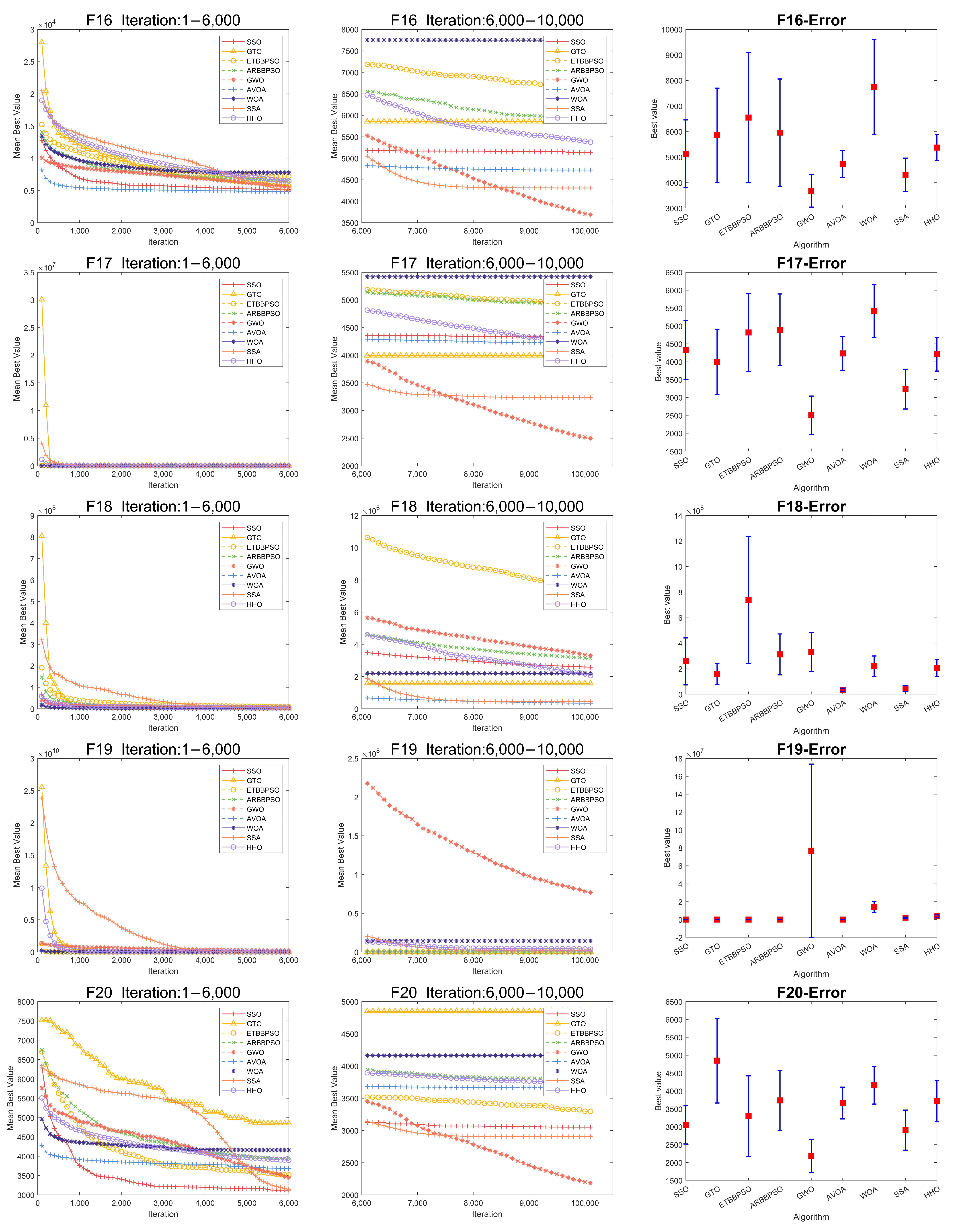
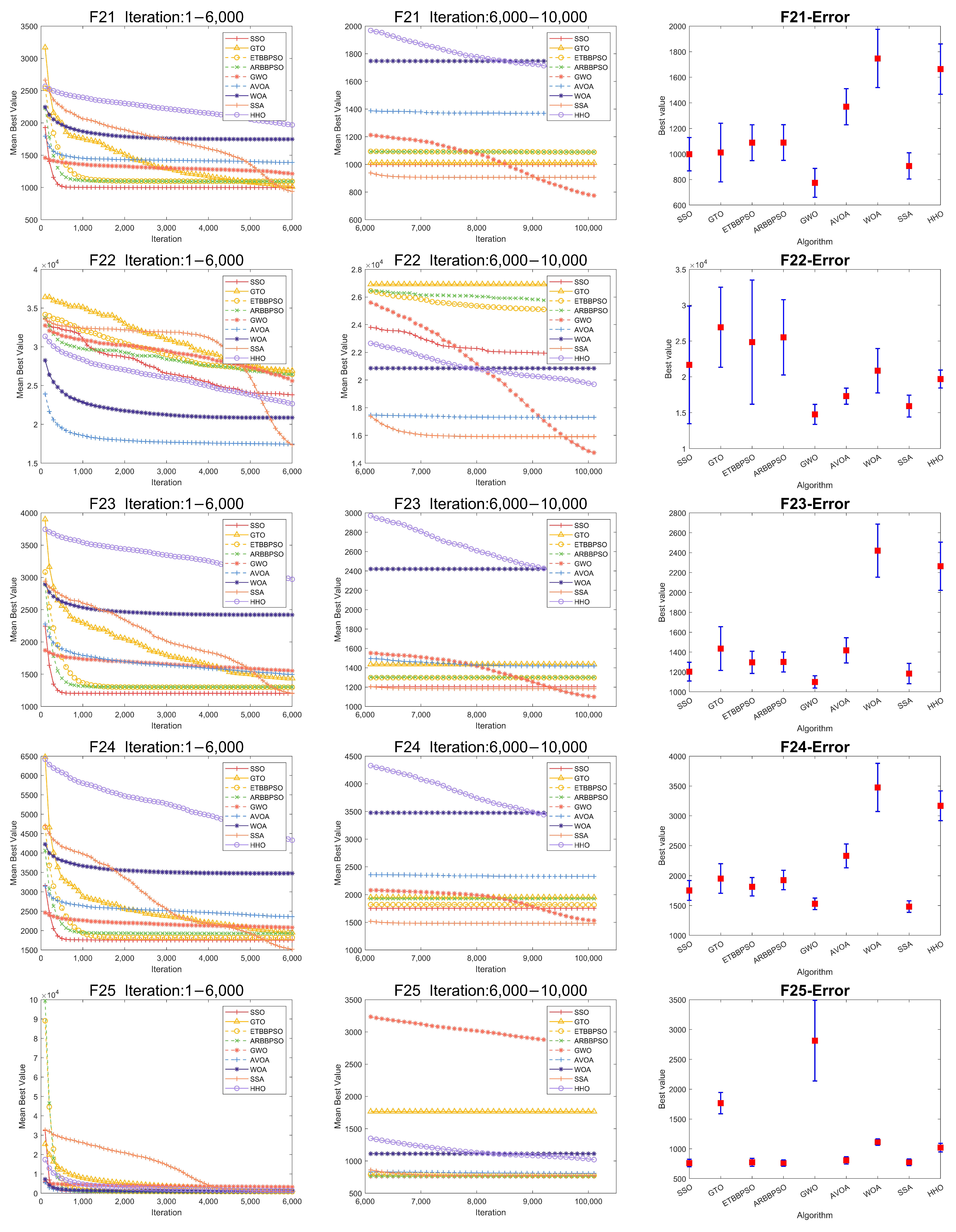
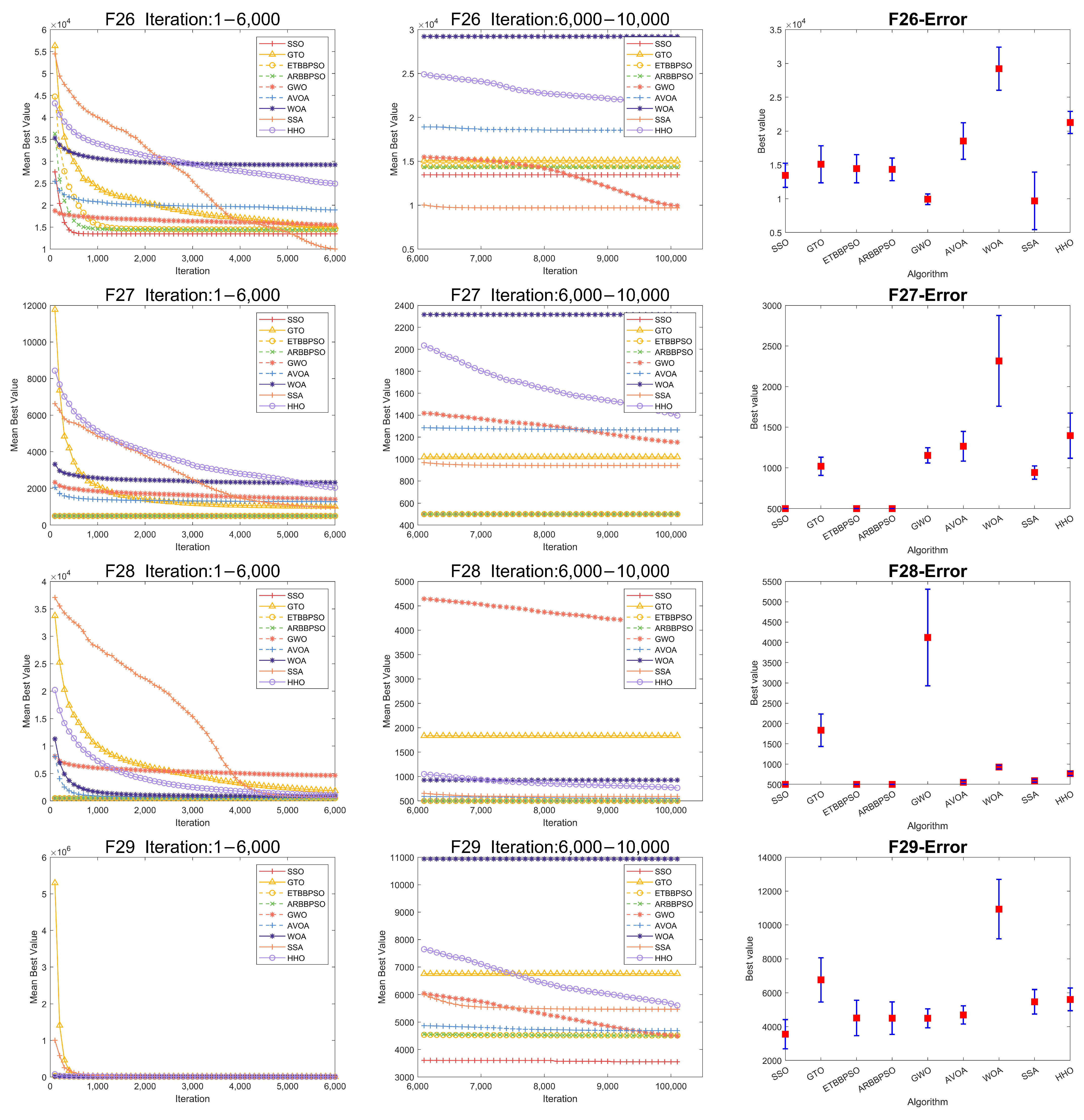
4. Results
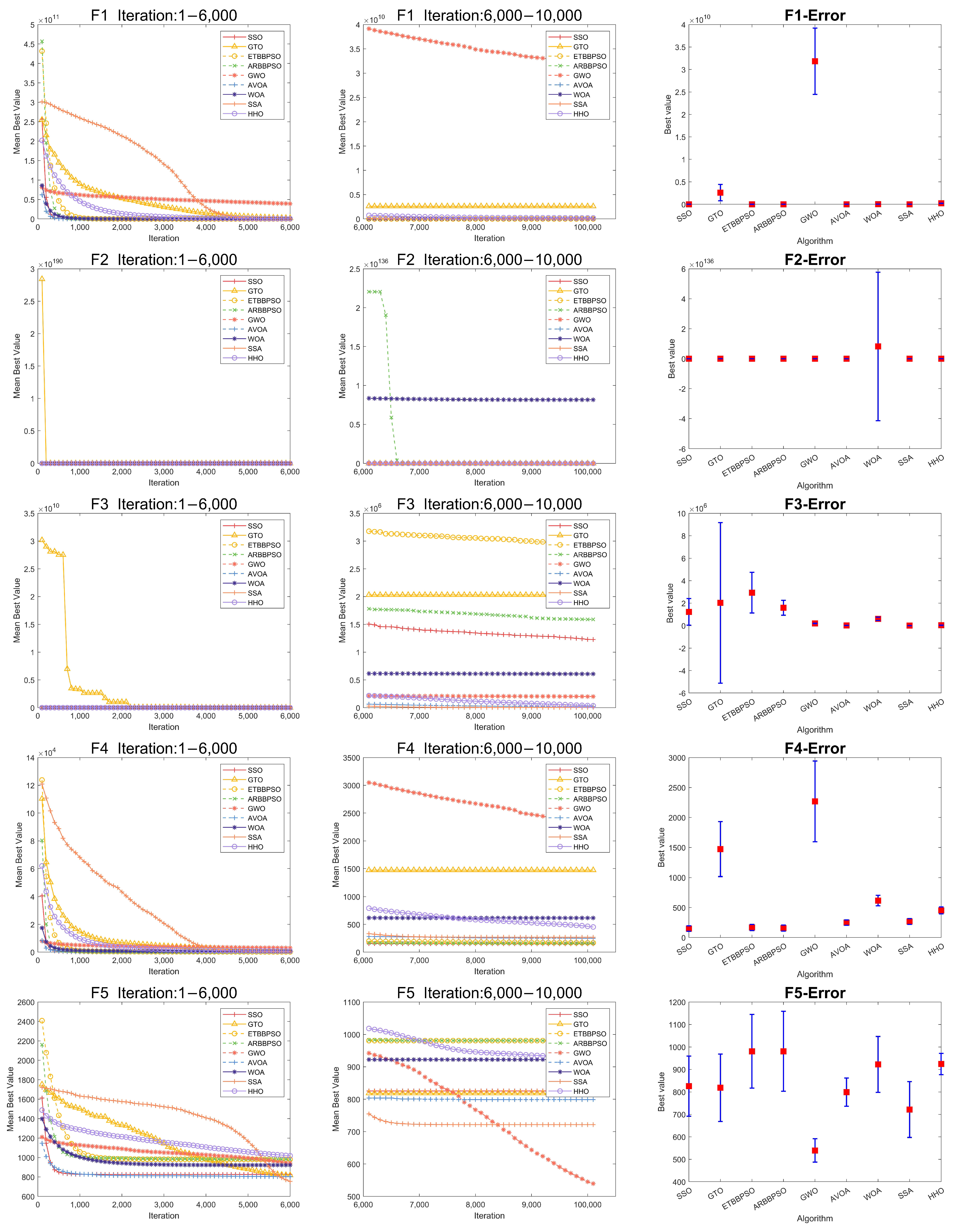
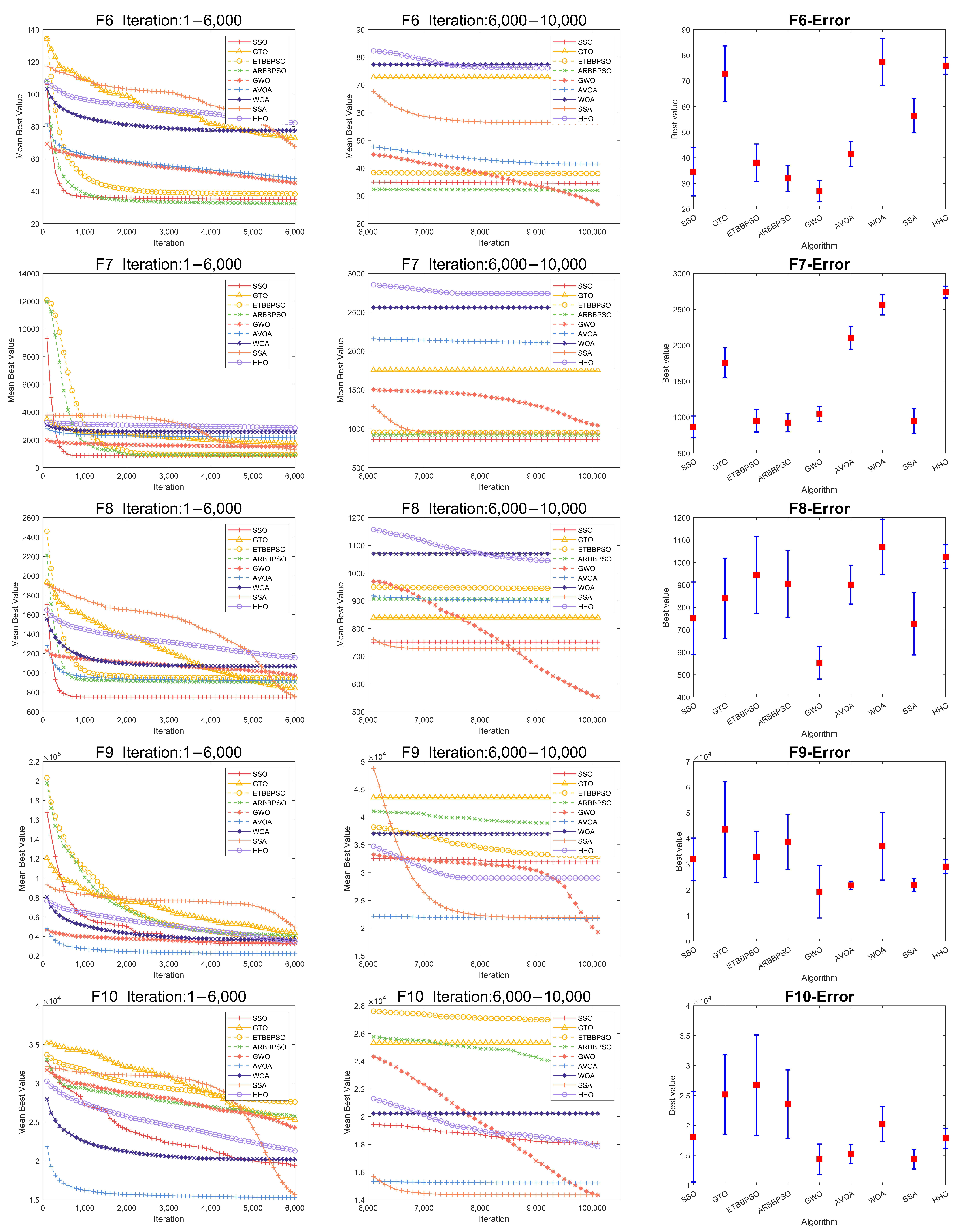
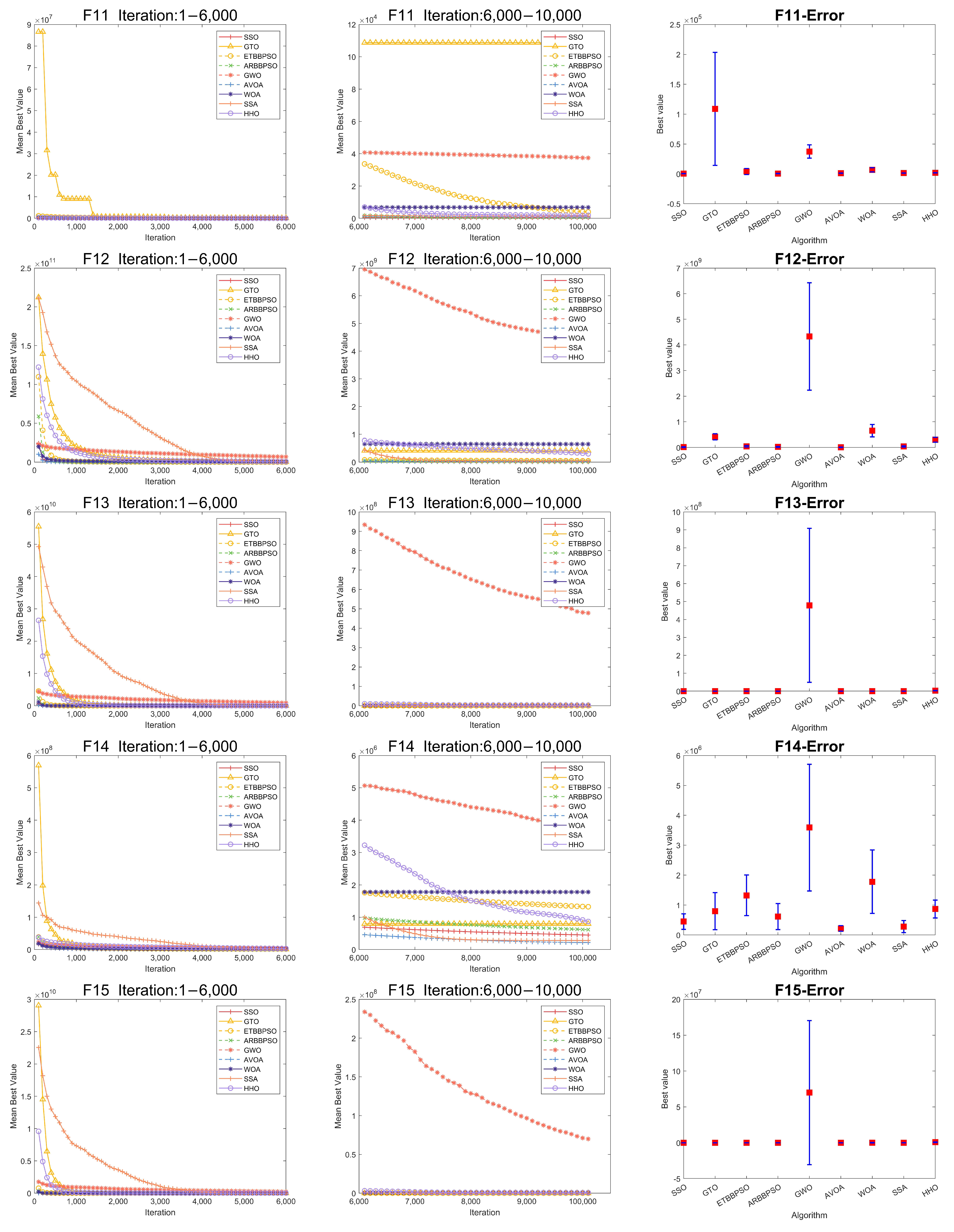
4.1. Numerical Experiments with CEC2017
- Unimodal Functions, ;
- Simple Multimodal Functions, ;
- Hybrid Functions, ;
- Composition Functions, .
- Population size for all algorithms, 100;
- Max iteration times, 1.000 ;
- Dimension, 100;
- Individual runs, 37.
- search range, [−100, +100]
Numerical Analysis
- In , The rank of SSO is 3, the first method is AVOA, the difference between the two methods is 76.174%;
- In , The rank of SSO is 3, the first method is AVOA, the difference between the two methods is 100%;
- In , The rank of SSO is 6, the first method is AVOA, the difference between the two methods is 98.343%;
- In , The rank of SSO is 1, the second method is ARBBPSO, the difference between the two methods is 5.42%;
- In , The rank of SSO is 4, the first method is GWO, the difference between the two methods is 34.647%;
- In , The rank of SSO is 3, the first method is GWO, the difference between the two methods is 21.938%;
- In , The rank of SSO is 1, the second method is ARBBPSO, the difference between the two methods is 6.178%;
- In , The rank of SSO is 2, the first method is GWO, the difference between the two methods is 26.383%;
- In , The rank of SSO is 4, the first method is GWO, the difference between the two methods is 39.515%;
- In ,The rank of SSO is 5, the first method is GWO, the difference between the two methods is 20.694%;
- In , The rank of SSO is 1, the second method is ARBBPSO, the difference between the two methods is 14.329%;
- In , The rank of SSO is 2, the first method is AVOA, the difference between the two methods is 34.981%;
- In , The rank of SSO is 3, the first method is ETBBPSO, the difference between the two methods is 18.873%;
- In , The rank of SSO is 2, the first method is AVOA, the difference between the two methods is 51.522%;
- In , The rank of SSO is 1, the second method is ETBBPSO, the difference between the two methods is 14.277%;
- In , The rank of SSO is 3, the first method is GWO, the difference between the two methods is 28.221%;
- In , The rank of SSO is 5, the first method is GWO, the difference between the two methods is 42.281%;
- In , The rank of SSO is 5, the first method is AVOA, the difference between the two methods is 86.234%;
- In , The rank of SSO is 1, the second method is ARBBPSO, the difference between the two methods is 27.192%;
- In , The rank of SSO is 2, the first method is GWO, the difference between the two methods is 28.455%;
- In , The rank of SSO is 2, the first method is GWO, the difference between the two methods is 22.436%;
- In , The rank of SSO is 6, the first method is GWO, the difference between the two methods is 31.869%;
- In , The rank of SSO is 2, the first method is GWO, the difference between the two methods is 8.565%;
- In , The rank of SSO is 2, the first method is GWO, the difference between the two methods is 12.753%;
- In , The rank of SSO is 2, the first method is ARBBPSO, the difference between the two methods is 0.131%;
- In , The rank of SSO is 2, the first method is GWO, the difference between the two methods is 26.263%;
- In , The rank of SSO is 1, the second method is ARBBPSO, the difference between the two methods is 0%;
- In ,The rank of SSO is 1, the second method is ARBBPSO, the difference between the two methods is 0%;
- In , The rank of SSO is 1, the second method is GWO, the difference between the two methods is 20.934%;
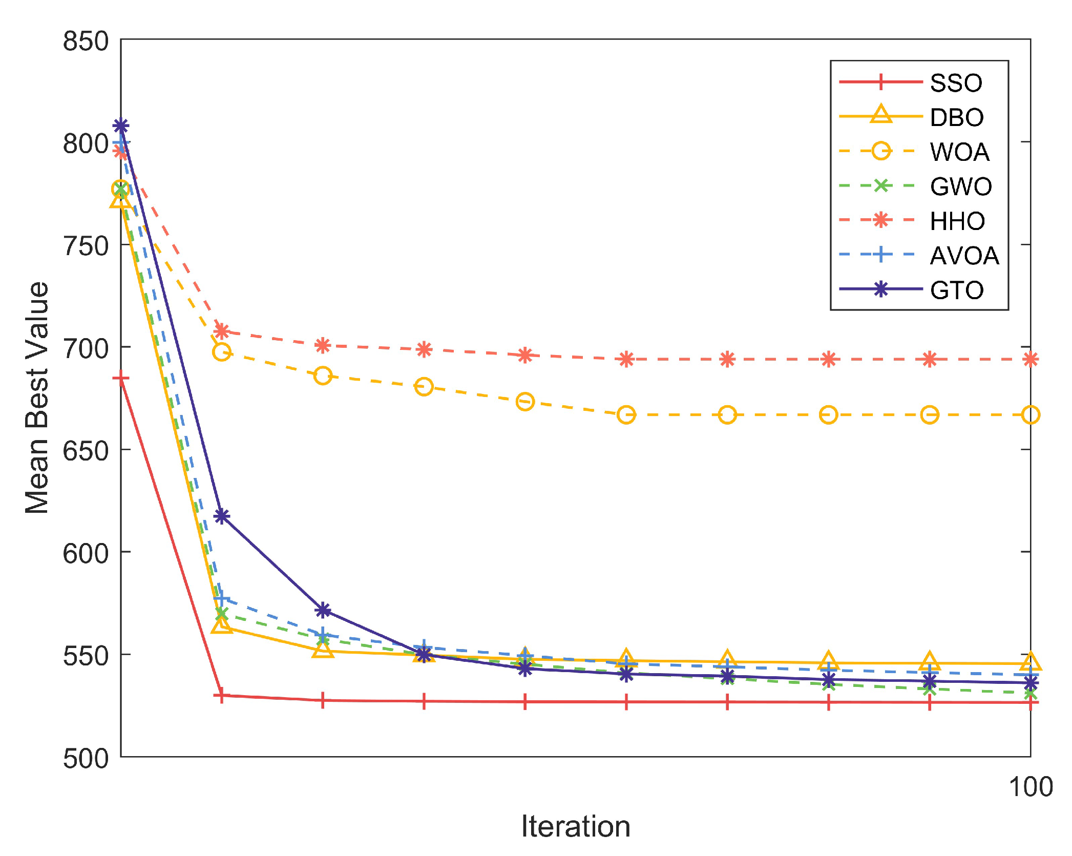
4.2. Numerical Experiments with CEC2022
4.3. Optimization Problem Formulation for Deep-Sea Probe Design
- : Wall thickness of the cylindrical section,
- : Wall thickness of the end caps,
- r: Radius of the probe,
- l: Length of the probe,
- : Material density,
- : Maximum internal pressure capacity,
- : Battery energy storage,
- : Sensor diameter.
4.4. Discussion
5. Conclusions
Author Contributions
Funding
Institutional Review Board Statement
Informed Consent Statement
Data Availability Statement
Conflicts of Interest
References
- Petrovic, A.; Damaševičius, R.; Jovanovic, L.; Toskovic, A.; Simic, V.; Bacanin, N.; Zivkovic, M.; Spalević, P. Marine Vessel Classification and Multivariate Trajectories Forecasting Using Metaheuristics-Optimized eXtreme Gradient Boosting and Recurrent Neural Networks. Appl. Sci. 2023, 13, 9181. [Google Scholar] [CrossRef]
- Yaseen, Z.M.; Melini Wan Mohtar, W.H.; Homod, R.Z.; Alawi, O.A.; Abba, S.I.; Oudah, A.Y.; Togun, H.; Goliatt, L.; Ul Hassan Kazmi, S.S.; Tao, H. Heavy metals prediction in coastal marine sediments using hybridized machine learning models with metaheuristic optimization algorithm. Chemosphere 2024, 352, 141329. [Google Scholar] [CrossRef] [PubMed]
- Zhang, Y.H.; Wang, X.J.; Zhang, X.Z.; Saad, M.; Zhao, R.J. Numerical Investigation of the Impacts of Large Particles on the Turbulent Flow and Surface Wear in Series-Connected Bends. J. Mar. Sci. Eng. 2024, 12, 164. [Google Scholar] [CrossRef]
- Nguyen, T.H.H.; Hou, T.H.; Pham, H.A.; Tsai, C.C. Oil Spill Sensitivity Analysis of the Coastal Waters of Taiwan Using an Integrated Modelling Approach. J. Mar. Sci. Eng. 2024, 12, 155. [Google Scholar] [CrossRef]
- Xing, R.; Zhang, Y.; Feng, Y.; Ji, F. Performance Analysis of a WPCN-Based Underwater Acoustic Communication System. J. Mar. Sci. Eng. 2023, 12, 43. [Google Scholar] [CrossRef]
- Kennedy, J.; Eberhart, R. Particle swarm optimization. In Proceedings of the ICNN’95—International Conference on Neural Networks, Perth, Australia, 27 November–1 December 1995; Volume 4, pp. 942–1948. [Google Scholar] [CrossRef]
- Fister, I.; Yang, X.S.; Brest, J. A comprehensive review of firefly algorithms. Swarm Evol. Comput. 2013, 13, 34–46. [Google Scholar] [CrossRef]
- Zhou, X.G.; Zhang, G.J. Differential evolution with underestimation-based multimutation strategy. IEEE Trans. Cybern. 2019, 49, 1353–1364. [Google Scholar] [CrossRef] [PubMed]
- Chen, L.; Liu, Y.; Gao, Y.; Wang, J. Carbon Emission Trading Policy and Carbon Emission Efficiency: An Empirical Analysis of China’s Prefecture-Level Cities. Front. Energy Res. 2021, 9, 793601. [Google Scholar] [CrossRef]
- Zhang, X.; Zou, D.; Shen, X. A novel simple particle swarm optimization algorithm for global optimization. Mathematics 2018, 6, 287. [Google Scholar] [CrossRef]
- Qiao, J.; Zhou, H.; Yang, C. Bare-Bones Multiobjective Particle Swarm Optimization Based on Parallel Cell Balanceable Fitness Estimation. IEEE Access 2018, 6, 32493–32506. [Google Scholar] [CrossRef]
- Zhang, X.; Melbourne, S.; Sarkar, C.; Chiaradia, A.; Webster, C. Effects of green space on walking: Does size, shape and density matter? Urban Stud. 2020, 57, 3402–3420. [Google Scholar] [CrossRef]
- Singh, G.; Singh, A. A hybrid algorithm using particle swarm optimization for solving transportation problem. Neural Comput. Appl. 2020, 32, 11699–11716. [Google Scholar] [CrossRef]
- Meng, X.; Li, J.; Member, S.; Dai, X.; Dou, J. Variable Neighborhood Search for a Colored Traveling Salesman Problem. IEEE Trans. Intell. Transp. Syst. 2018, 19, 1018–1026. [Google Scholar] [CrossRef]
- Meng, X.; Li, J.; Member, S.; Zhou, M.; Dai, X.; Dou, J. Population-Based Incremental Learning Algorithm for a Serial Colored Traveling Salesman Problem. IEEE Trans. Syst. Man, Cybern. Syst. 2018, 48, 277–288. [Google Scholar] [CrossRef]
- Al-Andoli, M.; Tan, S.C.; Cheah, W.P. Parallel stacked autoencoder with particle swarm optimization for community detection in complex networks. Appl. Intell. 2022, 52, 3366–3386. [Google Scholar] [CrossRef]
- Ahandani, M.A.; Abbasfam, J.; Kharrati, H. Parameter identification of permanent magnet synchronous motors using quasi-opposition-based particle swarm optimization and hybrid chaotic particle swarm optimization algorithms. Appl. Intell. 2022, 52, 13082–13096. [Google Scholar] [CrossRef]
- Zhang, J.; Zhao, X.; Jin, S.; Greaves, D. Phase-resolved real-time ocean wave prediction with quantified uncertainty based on variational Bayesian machine learning. Appl. Energy 2022, 324, 119711. [Google Scholar] [CrossRef]
- Hu, P.; Pan, J.S.; Chu, S.C.; Sun, C. Multi-surrogate assisted binary particle swarm optimization algorithm and its application for feature selection. Appl. Soft Comput. 2022, 121, 108736. [Google Scholar] [CrossRef]
- Wang, H.; Zhang, Z. Forecasting Chinese provincial carbon emissions using a novel grey prediction model considering spatial correlation. Expert Syst. Appl. 2022, 209, 118261. [Google Scholar] [CrossRef]
- Lu, B.; Zhou, C. Particle Swarm Algorithm and Its Application in Tourism Route Design and Optimization. Comput. Intell. Neurosci. 2022, 2022, 6467086. [Google Scholar] [CrossRef]
- Pan, J.; Bardhan, R. Evaluating the risk of accessing green spaces in COVID-19 pandemic: A model for public urban green spaces (PUGS) in London. Urban For. Urban Green. 2022, 74, 127648. [Google Scholar] [CrossRef] [PubMed]
- Gao, Y.; Du, W.; Yan, G. Selectively-informed particle swarm optimization. Sci. Rep. 2015, 5, 9295. [Google Scholar] [CrossRef] [PubMed]
- Liang, X.; Li, W.; Zhang, Y.; Zhou, M. An adaptive particle swarm optimization method based on clustering. Soft Comput. 2015, 19, 431–448. [Google Scholar] [CrossRef]
- Li, J.; Zhang, J.; Jiang, C.; Zhou, M. Composite Particle Swarm Optimizer with Historical Memory for Function Optimization. IEEE Trans. Cybern. 2015, 45, 2350–2363. [Google Scholar] [CrossRef]
- Pornsing, C.; Sodhi, M.S.; Lamond, B.F. Novel self-adaptive particle swarm optimization methods. Soft Comput. 2016, 20, 3579–3593. [Google Scholar] [CrossRef]
- Guo, J.; Sato, Y. A pair-wise bare bones particle swarm optimization algorithm. In Proceedings of the 2017 IEEE/ACIS 16th International Conference on Computer and Information Science (ICIS), Wuhan, China, 24–26 May 2017; Number 1. pp. 353–358. [Google Scholar] [CrossRef]
- Guo, J.; Sato, Y. A Bare Bones Particle Swarm Optimization Algorithm with Dynamic Local Search. In Advances in Swarm Intelligence: 8th International Conference, ICSI 2017, Fukuoka, Japan, 27 July–1 August 2017, Proceedings, Part I; Tan, Y., Takagi, H., Shi, Y., Eds.; Springer International Publishing: Cham, Switzerland, 2017; pp. 158–165. [Google Scholar] [CrossRef]
- Guo, J.; Sato, Y. A Hierarchical Bare Bones Particle Swarm Optimization Algorithm. In Proceedings of the 2017 IEEE International Conference on Systems, Man, and Cybernetics (SMC), Banff, AB, Canada, 5–8 October 2017; pp. 1936–1941. [Google Scholar] [CrossRef]
- Kennedy, J. Bare bones particle swarms. In Proceedings of the 2003 IEEE Swarm Intelligence Symposium, SIS’03 (Cat. No.03EX706), Indianapolis, IN, USA, 26 April 2003; pp. 80–87. [Google Scholar] [CrossRef]
- Xu, X.; Rong, H.; Trovati, M.; Liptrott, M.; Bessis, N. CS-PSO: Chaotic particle swarm optimization algorithm for solving combinatorial optimization problems. Soft Comput. 2018, 22, 783–795. [Google Scholar] [CrossRef]
- Tian, D.; Shi, Z. MPSO: Modified particle swarm optimization and its applications. Swarm Evol. Comput. 2018, 41, 49–68. [Google Scholar] [CrossRef]
- Ghasemi, M.; Akbari, E.; Rahimnejad, A.; Razavi, S.E.; Ghavidel, S.; Li, L. Phasor particle swarm optimization: A simple and efficient variant of PSO. Soft Comput. 2019, 23, 9701–9718. [Google Scholar] [CrossRef]
- Guo, J.; Sato, Y. A fission-fusion hybrid bare bones particle swarm optimization algorithm for single-objective optimization problems. Appl. Intell. 2019, 49, 3641–3651. [Google Scholar] [CrossRef]
- Xu, G.; Cui, Q.; Shi, X.; Ge, H.; Zhan, Z.H.; Lee, H.P.; Liang, Y.; Tai, R.; Wu, C. Particle swarm optimization based on dimensional learning strategy. Swarm Evol. Comput. 2019, 45, 33–51. [Google Scholar] [CrossRef]
- Xu, Y.; Pi, D. A reinforcement learning-based communication topology in particle swarm optimization. Neural Comput. Appl. 2020, 32, 10007–10032. [Google Scholar] [CrossRef]
- Yamanaka, Y.; Yoshida, K. Simple gravitational particle swarm algorithm for multimodal optimization problems. PLoS ONE 2021, 16, e0248470. [Google Scholar] [CrossRef] [PubMed]
- Liu, J.; Jin, B.; Yang, J.; Xu, L. Sea surface temperature prediction using a cubic B-spline interpolation and spatiotemporal attention mechanism. Remote Sens. Lett. 2021, 12, 478–487. [Google Scholar] [CrossRef]
- Wang, Z.J.; Zhan, Z.H.; Kwong, S.; Jin, H.; Zhang, J. Adaptive Granularity Learning Distributed Particle Swarm Optimization for Large-Scale Optimization. IEEE Trans. Cybern. 2021, 51, 1175–1188. [Google Scholar] [CrossRef] [PubMed]
- Li, X.; Wang, Z.; Ying, Y.; Xiao, F. Multipopulation Particle Swarm Optimization Algorithm with Neighborhood Learning. Sci. Program. 2022, 2022, 8312450. [Google Scholar] [CrossRef]
- Tian, H.; Guo, J.; Xiao, H.; Yan, K.; Sato, Y. An electronic transition-based bare bones particle swarm optimization algorithm for high dimensional optimization problems. PLoS ONE 2022, 17, e0271925. [Google Scholar] [CrossRef]
- Guo, Q.; Su, Z.; Chiao, C. Carbon emissions trading policy, carbon finance, and carbon emissions reduction: Evidence from a quasi-natural experiment in China. Econ. Chang. Restruct. 2022, 55, 1445–1480. [Google Scholar] [CrossRef]
- Zhou, G.; Guo, J.; Yan, K.; Zhou, G.; Li, B. An Atomic Retrospective Learning Bare Bone Particle Swarm Optimization. In Advances in Swarm Intelligence. ICSI 2023; Lecture Notes in Computer Science; Springer: Cham, Switzerland, 2023; Volume 13968, pp. 168–179. [Google Scholar] [CrossRef]
- Xue, J.; Shen, B. Dung beetle optimizer: A new meta-heuristic algorithm for global optimization. J. Supercomput. 2023, 79, 7305–7336. [Google Scholar] [CrossRef]
- Mirjalili, S.; Lewis, A. The Whale Optimization Algorithm. Adv. Eng. Softw. 2016, 95, 51–67. [Google Scholar] [CrossRef]
- Mirjalili, S.; Mirjalili, S.M.; Lewis, A. Grey Wolf Optimizer. Adv. Eng. Softw. 2014, 69, 46–61. [Google Scholar] [CrossRef]
- Heidari, A.A.; Mirjalili, S.; Faris, H.; Aljarah, I.; Mafarja, M.; Chen, H. Harris hawks optimization: Algorithm and applications. Future Gener. Comput. Syst. 2019, 97, 849–872. [Google Scholar] [CrossRef]
- Abdollahzadeh, B.; Gharehchopogh, F.S.; Mirjalili, S. African vultures optimization algorithm: A new nature-inspired metaheuristic algorithm for global optimization problems. Comput. Ind. Eng. 2021, 158, 107408. [Google Scholar] [CrossRef]
- Abdollahzadeh, B.; Soleimanian Gharehchopogh, F.; Mirjalili, S. Artificial gorilla troops optimizer: A new nature-inspired metaheuristic algorithm for global optimization problems. Int. J. Intell. Syst. 2021, 36, 22535. [Google Scholar] [CrossRef]

| F | Type | SSO | DBO | WOA | GWO | HHO | AVOA | GTO | ARBBPSO | ETBBPSO |
|---|---|---|---|---|---|---|---|---|---|---|
| 1 | Mean | 2.808 × 10⁴ | 5.748 × 10⁷ | 3.515 × 10⁷ | 3.184 × 10¹⁰ | 2.097 × 10⁸ | 6.690 × 10³ | 2.604 × 10⁹ | 2.912 × 10⁴ | 1.656 × 10⁴ |
| Std | 2.760 × 10⁴ | 3.705 × 10⁷ | 1.173 × 10⁷ | 7.385 × 10⁹ | 2.181 × 10⁷ | 9.224 × 10³ | 1.822 × 10⁹ | 3.091 × 10⁴ | 2.186 × 10⁴ | |
| Best | 1.851 × 101 | 1.490 × 10⁶ | 1.560 × 10⁷ | 2.009 × 10¹⁰ | 1.621 × 10⁸ | 9.860 × 100 | 7.170 × 10⁸ | 1.369 × 10² | 4.990 × 100 | |
| Worst | 8.870 × 10⁴ | 1.431 × 10⁸ | 7.225 × 10⁷ | 5.204 × 10¹⁰ | 2.517 × 10⁸ | 3.450 × 10⁴ | 8.877 × 10⁹ | 1.281 × 10⁵ | 1.120 × 10⁵ | |
| Rank | 3 | 6 | 5 | 9 | 7 | 1 | 8 | 4 | 2 | |
| 2 | Mean | 1.909 × 1089 | 1.845 × 10134 | 8.159 × 10135 | 6.547 × 10125 | 1.117 × 1073 | 1.326 × 1030 | 3.553 × 10119 | 9.078 × 10125 | 7.782 × 10114 |
| Std | 7.879 × 1089 | 1.122 × 10135 | 4.955 × 10136 | 3.976 × 10126 | 5.615 × 1073 | 5.600 × 1030 | 1.423 × 10120 | 5.522 × 10126 | 3.073 × 10115 | |
| Best | 1.679 × 1068 | 2.434 × 1098 | 2.676 × 10110 | 5.418 × 1097 | 6.231 × 1059 | 3.731 × 10¹³ | 9.303 × 1099 | 6.574 × 1084 | 2.233 × 1088 | |
| Worst | 4.579 × 1090 | 6.822 × 10135 | 3.014 × 10137 | 2.418 × 10127 | 3.375 × 1074 | 2.681 × 1031 | 7.773 × 10120 | 3.359 × 10127 | 1.718 × 10116 | |
| Rank | 3 | 8 | 9 | 6 | 2 | 1 | 5 | 7 | 4 | |
| 3 | Mean | 1.227 × 10⁶ | 3.241 × 10⁵ | 6.068 × 10⁵ | 2.008 × 10⁵ | 3.406 × 10⁴ | 2.034 × 10⁴ | 2.030 × 10⁶ | 1.589 × 10⁶ | 2.934 × 10⁶ |
| Std | 1.186 × 10⁶ | 1.856 × 10⁴ | 1.497 × 10⁵ | 1.767 × 10⁴ | 8.364 × 10³ | 6.828 × 10³ | 7.150 × 10⁶ | 6.647 × 10⁵ | 1.808 × 10⁶ | |
| Best | 4.535 × 10⁵ | 2.578 × 10⁵ | 3.368 × 10⁵ | 1.638 × 10⁵ | 1.796 × 10⁴ | 8.612 × 10³ | 2.438 × 10⁵ | 6.560 × 10⁵ | 1.059 × 10⁶ | |
| Worst | 4.888 × 10⁶ | 3.516 × 10⁵ | 8.400 × 10⁵ | 2.421 × 10⁵ | 5.648 × 10⁴ | 3.839 × 10⁴ | 4.276 × 10⁷ | 3.261 × 10⁶ | 8.476 × 10⁶ | |
| Rank | 6 | 4 | 5 | 3 | 2 | 1 | 8 | 7 | 9 | |
| 4 | Mean | 1.493 × 10² | 4.300 × 10² | 6.164 × 10² | 2.268 × 10³ | 4.530 × 10² | 2.495 × 10² | 1.473 × 10³ | 1.578 × 10² | 1.683 × 10² |
| Std | 4.601 × 101 | 7.513 × 101 | 8.827 × 101 | 6.743 × 10² | 5.750 × 101 | 4.472 × 101 | 4.581 × 10² | 5.156 × 101 | 5.145 × 101 | |
| Best | 8.963 × 101 | 2.765 × 10² | 4.498 × 10² | 1.096 × 10³ | 3.622 × 10² | 1.930 × 10² | 7.983 × 10² | 7.623 × 101 | 7.982 × 101 | |
| Worst | 2.934 × 10² | 5.789 × 10² | 8.222 × 10² | 4.021 × 10³ | 5.927 × 10² | 3.663 × 10² | 2.757 × 10³ | 3.117 × 10² | 2.893 × 10² | |
| Rank | 1 | 5 | 7 | 9 | 6 | 4 | 8 | 2 | 3 | |
| 5 | Mean | 8.255 × 10² | 1.089 × 10³ | 9.223 × 10² | 5.395 × 10² | 9.242 × 10² | 7.989 × 10² | 8.184 × 10² | 9.809 × 10² | 9.808 × 10² |
| Std | 1.336 × 10² | 1.545 × 10² | 1.244 × 10² | 5.188 × 101 | 4.758 × 101 | 6.290 × 101 | 1.499 × 10² | 1.781 × 10² | 1.639 × 10² | |
| Best | 5.462 × 10² | 8.141 × 10² | 7.312 × 10² | 4.092 × 10² | 8.221 × 10² | 6.398 × 10² | 6.021 × 10² | 6.248 × 10² | 6.706 × 10² | |
| Worst | 1.081 × 10³ | 1.361 × 10³ | 1.250 × 10³ | 6.650 × 10² | 1.038 × 10³ | 9.522 × 10² | 1.393 × 10³ | 1.369 × 10³ | 1.270 × 10³ | |
| Rank | 4 | 9 | 5 | 1 | 6 | 2 | 3 | 8 | 7 | |
| 6 | Mean | 3.455 × 101 | 7.188 × 101 | 7.737 × 101 | 2.697 × 101 | 7.590 × 101 | 4.148 × 101 | 7.272 × 101 | 3.194 × 101 | 3.806 × 101 |
| Std | 9.455 × 100 | 9.560 × 100 | 9.166 × 100 | 4.047 × 100 | 3.312 × 100 | 4.854 × 100 | 1.090 × 101 | 5.052 × 100 | 7.284 × 100 | |
| Best | 1.108 × 101 | 5.496 × 101 | 6.168 × 101 | 1.967 × 101 | 6.720 × 101 | 3.192 × 101 | 4.958 × 101 | 1.972 × 101 | 2.120 × 101 | |
| Worst | 5.381 × 101 | 9.361 × 101 | 1.048 × 10² | 3.501 × 101 | 8.179 × 101 | 5.283 × 101 | 9.305 × 101 | 4.202 × 101 | 5.119 × 101 | |
| Rank | 3 | 6 | 9 | 1 | 8 | 5 | 7 | 2 | 4 | |
| 7 | Mean | 8.635 × 10² | 1.507 × 10³ | 2.561 × 10³ | 1.044 × 10³ | 2.740 × 10³ | 2.101 × 10³ | 1.754 × 10³ | 9.204 × 10² | 9.485 × 10² |
| Std | 1.510 × 10² | 3.905 × 10² | 1.393 × 10² | 1.037 × 10² | 8.270 × 101 | 1.582 × 10² | 2.081 × 10² | 1.256 × 10² | 1.575 × 10² | |
| Best | 6.102 × 10² | 1.036 × 10³ | 2.212 × 10³ | 8.211 × 10² | 2.560 × 10³ | 1.773 × 10³ | 1.337 × 10³ | 6.931 × 10² | 6.999 × 10² | |
| Worst | 1.147 × 10³ | 3.145 × 10³ | 2.894 × 10³ | 1.309 × 10³ | 2.932 × 10³ | 2.442 × 10³ | 2.239 × 10³ | 1.212 × 10³ | 1.326 × 10³ | |
| Rank | 1 | 5 | 8 | 4 | 9 | 7 | 6 | 2 | 3 | |
| 8 | Mean | 7.509 × 10² | 1.143 × 10³ | 1.069 × 10³ | 5.528 × 10² | 1.026 × 10³ | 9.013 × 10² | 8.395 × 10² | 9.049 × 10² | 9.439 × 10² |
| Std | 1.620 × 10² | 1.525 × 10² | 1.231 × 10² | 7.252 × 101 | 5.340 × 101 | 8.687 × 101 | 1.798 × 10² | 1.495 × 10² | 1.705 × 10² | |
| Best | 5.174 × 10² | 7.631 × 10² | 8.041 × 10² | 4.036 × 10² | 8.413 × 10² | 7.323 × 10² | 5.891 × 10² | 5.801 × 10² | 5.612 × 10² | |
| Worst | 1.132 × 10³ | 1.405 × 10³ | 1.476 × 10³ | 7.012 × 10² | 1.108 × 10³ | 1.102 × 10³ | 1.533 × 10³ | 1.296 × 10³ | 1.223 × 10³ | |
| Rank | 2 | 9 | 8 | 1 | 7 | 4 | 3 | 5 | 6 |
| F | Type | SSO | DBO | WOA | GWO | HHO | AVOA | GTO | ARBBPSO | ETBBPSO |
|---|---|---|---|---|---|---|---|---|---|---|
| 9 | Mean | 3.189 × 10⁴ | 3.533 × 10⁴ | 3.694 × 10⁴ | 1.929 × 10⁴ | 2.902 × 10⁴ | 2.176 × 10⁴ | 4.350 × 10⁴ | 3.872 × 10⁴ | 3.285 × 10⁴ |
| Std | 8.257 × 10³ | 9.423 × 10³ | 1.313 × 10⁴ | 1.023 × 10⁴ | 2.590 × 10³ | 1.672 × 10³ | 1.855 × 10⁴ | 1.076 × 10⁴ | 1.002 × 10⁴ | |
| Best | 1.398 × 10⁴ | 1.751 × 10⁴ | 2.303 × 10⁴ | 9.616 × 10³ | 2.394 × 10⁴ | 1.901 × 10⁴ | 2.294 × 10⁴ | 1.777 × 10⁴ | 1.762 × 10⁴ | |
| Worst | 4.255 × 10⁴ | 4.880 × 10⁴ | 8.197 × 10⁴ | 4.220 × 10⁴ | 3.367 × 10⁴ | 2.774 × 10⁴ | 7.876 × 10⁴ | 8.490 × 10⁴ | 4.980 × 10⁴ | |
| Rank | 4 | 6 | 7 | 1 | 3 | 2 | 9 | 8 | 5 | |
| 10 | Mean | 1.808 × 10⁴ | 1.735 × 10⁴ | 2.023 × 10⁴ | 1.434 × 10⁴ | 1.783 × 10⁴ | 1.521 × 10⁴ | 2.516 × 10⁴ | 2.355 × 10⁴ | 2.671 × 10⁴ |
| Std | 7.565 × 10³ | 1.543 × 10³ | 2.902 × 10³ | 2.535 × 10³ | 1.718 × 10³ | 1.573 × 10³ | 6.647 × 10³ | 5.728 × 10³ | 8.382 × 10³ | |
| Best | 1.069 × 10⁴ | 1.446 × 10⁴ | 1.545 × 10⁴ | 1.057 × 10⁴ | 1.334 × 10⁴ | 1.213 × 10⁴ | 1.270 × 10⁴ | 1.233 × 10⁴ | 9.839 × 10³ | |
| Worst | 3.297 × 10⁴ | 2.025 × 10⁴ | 2.601 × 10⁴ | 2.693 × 10⁴ | 2.084 × 10⁴ | 1.979 × 10⁴ | 3.375 × 10⁴ | 2.947 × 10⁴ | 3.364 × 10⁴ | |
| Rank | 5 | 3 | 6 | 1 | 4 | 2 | 8 | 7 | 9 | |
| 11 | Mean | 4.957 × 10² | 1.867 × 10⁴ | 6.803 × 10³ | 3.741 × 10⁴ | 1.861 × 10³ | 1.202 × 10³ | 1.087 × 10⁵ | 5.786 × 10² | 3.974 × 10³ |
| Std | 1.357 × 10² | 3.081 × 10⁴ | 3.448 × 10³ | 1.107 × 10⁴ | 1.889 × 10² | 2.255 × 10² | 9.458 × 10⁴ | 2.244 × 10² | 5.112 × 10³ | |
| Best | 2.573 × 10² | 2.700 × 10³ | 4.322 × 10³ | 1.755 × 10⁴ | 1.512 × 10³ | 7.107 × 10² | 2.676 × 10⁴ | 2.266 × 10² | 3.565 × 10² | |
| Worst | 7.958 × 10² | 1.483 × 10⁵ | 2.567 × 10⁴ | 6.831 × 10⁴ | 2.247 × 10³ | 1.602 × 10³ | 5.289 × 10⁵ | 1.058 × 10³ | 2.318 × 10⁴ | |
| Rank | 1 | 7 | 6 | 8 | 4 | 3 | 9 | 2 | 5 | |
| 12 | Mean | 1.830 × 10⁷ | 4.235 × 10⁸ | 6.533 × 10⁸ | 4.330 × 10⁹ | 3.029 × 10⁸ | 1.190 × 10⁷ | 4.165 × 10⁸ | 2.783 × 10⁷ | 4.958 × 10⁷ |
| Std | 1.196 × 10⁷ | 2.298 × 10⁸ | 2.408 × 10⁸ | 2.095 × 10⁹ | 9.060 × 10⁷ | 6.478 × 10⁶ | 1.147 × 10⁸ | 1.477 × 10⁷ | 2.681 × 10⁷ | |
| Best | 6.615 × 10⁶ | 7.719 × 10⁷ | 2.185 × 10⁸ | 1.473 × 10⁹ | 1.635 × 10⁸ | 3.719 × 10⁶ | 2.026 × 10⁸ | 7.105 × 10⁶ | 5.747 × 10⁶ | |
| Worst | 5.860 × 10⁷ | 9.782 × 10⁸ | 1.079 × 10⁹ | 9.595 × 10⁹ | 5.550 × 10⁸ | 2.737 × 10⁷ | 7.120 × 10⁸ | 8.331 × 10⁷ | 1.144 × 10⁸ | |
| Rank | 2 | 7 | 8 | 9 | 5 | 1 | 6 | 3 | 4 | |
| 13 | Mean | 9.419 × 10³ | 9.405 × 10⁶ | 9.002 × 10⁴ | 4.787 × 10⁸ | 3.105 × 10⁶ | 3.811 × 10⁴ | 3.234 × 10⁴ | 9.378 × 10³ | 7.642 × 10³ |
| Std | 1.186 × 10⁴ | 1.835 × 10⁷ | 3.417 × 10⁴ | 4.293 × 10⁸ | 5.306 × 10⁵ | 1.059 × 10⁴ | 1.306 × 10⁴ | 1.530 × 10⁴ | 1.233 × 10⁴ | |
| Best | 6.528 × 10² | 1.196 × 10⁵ | 4.051 × 10⁴ | 9.201 × 10⁴ | 2.014 × 10⁶ | 2.153 × 10⁴ | 1.419 × 10⁴ | 2.912 × 10² | 2.868 × 10² | |
| Worst | 3.599 × 10⁴ | 9.361 × 10⁷ | 1.596 × 10⁵ | 1.853 × 10⁹ | 4.130 × 10⁶ | 6.888 × 10⁴ | 6.511 × 10⁴ | 8.090 × 10⁴ | 4.816 × 10⁴ | |
| Rank | 3 | 8 | 6 | 9 | 7 | 5 | 4 | 2 | 1 | |
| 14 | Mean | 4.505 × 10⁵ | 3.598 × 10⁶ | 1.782 × 10⁶ | 3.591 × 10⁶ | 8.700 × 10⁵ | 2.184 × 10⁵ | 7.977 × 10⁵ | 6.176 × 10⁵ | 1.325 × 10⁶ |
| Std | 2.583 × 10⁵ | 3.441 × 10⁶ | 1.059 × 10⁶ | 2.115 × 10⁶ | 3.002 × 10⁵ | 9.406 × 10⁴ | 6.201 × 10⁵ | 4.363 × 10⁵ | 6.751 × 10⁵ | |
| Best | 1.425 × 10⁵ | 1.266 × 10⁵ | 4.800 × 10⁵ | 6.837 × 10⁵ | 3.137 × 10⁵ | 5.758 × 10⁴ | 9.775 × 10⁴ | 1.427 × 10⁵ | 4.959 × 10⁵ | |
| Worst | 1.131 × 10⁶ | 1.302 × 10⁷ | 4.792 × 10⁶ | 9.880 × 10⁶ | 1.634 × 10⁶ | 4.261 × 10⁵ | 3.816 × 10⁶ | 2.290 × 10⁶ | 2.803 × 10⁶ | |
| Rank | 2 | 9 | 7 | 8 | 5 | 1 | 4 | 3 | 6 | |
| 15 | Mean | 6.377 × 10³ | 7.555 × 10⁵ | 1.308 × 10⁵ | 7.000 × 10⁷ | 7.655 × 10⁵ | 2.200 × 10⁴ | 7.456 × 10³ | 7.748 × 10³ | 7.439 × 10³ |
| Std | 5.773 × 10³ | 1.481 × 10⁶ | 2.144 × 10⁵ | 1.005 × 10⁸ | 3.090 × 10⁵ | 7.872 × 10³ | 4.781 × 10³ | 1.019 × 10⁴ | 1.312 × 10⁴ | |
| Best | 1.849 × 10² | 4.700 × 10⁴ | 2.620 × 10⁴ | 4.352 × 10⁵ | 1.394 × 10⁵ | 6.418 × 10³ | 3.032 × 10³ | 1.612 × 10² | 1.635 × 10² | |
| Worst | 2.138 × 10⁴ | 7.265 × 10⁶ | 1.054 × 10⁶ | 3.816 × 10⁸ | 1.849 × 10⁶ | 4.234 × 10⁴ | 2.806 × 10⁴ | 4.044 × 10⁴ | 7.599 × 10⁴ | |
| Rank | 1 | 7 | 6 | 9 | 8 | 5 | 3 | 4 | 2 | |
| 16 | Mean | 5.132 × 10³ | 5.921 × 10³ | 7.751 × 10³ | 3.684 × 10³ | 5.377 × 10³ | 4.724 × 10³ | 5.854 × 10³ | 5.957 × 10³ | 6.546 × 10³ |
| Std | 1.326 × 10³ | 9.500 × 10² | 1.853 × 10³ | 6.423 × 10² | 5.029 × 10² | 5.282 × 10² | 1.846 × 10³ | 2.099 × 10³ | 2.552 × 10³ | |
| Best | 3.655 × 10³ | 3.863 × 10³ | 4.193 × 10³ | 2.205 × 10³ | 4.483 × 10³ | 3.733 × 10³ | 3.794 × 10³ | 3.357 × 10³ | 3.885 × 10³ | |
| Worst | 9.912 × 10³ | 7.955 × 10³ | 1.340 × 10⁴ | 4.936 × 10³ | 6.998 × 10³ | 6.212 × 10³ | 9.924 × 10³ | 1.031 × 10⁴ | 1.209 × 10⁴ | |
| Rank | 3 | 6 | 9 | 1 | 4 | 2 | 5 | 7 | 8 |
| F | Type | SSO | DBO | WOA | GWO | HHO | AVOA | GTO | ARBBPSO | ETBBPSO |
|---|---|---|---|---|---|---|---|---|---|---|
| 17 | Mean | 4.331 × 10³ | 5.316 × 10³ | 5.418 × 10³ | 2.500 × 10³ | 4.207 × 10³ | 4.230 × 10³ | 3.994 × 10³ | 4.892 × 10³ | 4.818 × 10³ |
| Std | 8.247 × 10² | 1.054 × 10³ | 7.340 × 10² | 5.376 × 10² | 4.684 × 10² | 4.697 × 10² | 9.162 × 10² | 1.001 × 10³ | 1.093 × 10³ | |
| Best | 2.686 × 10³ | 3.639 × 10³ | 4.328 × 10³ | 1.546 × 10³ | 3.531 × 10³ | 3.003 × 10³ | 2.678 × 10³ | 2.963 × 10³ | 3.252 × 10³ | |
| Worst | 6.121 × 10³ | 8.138 × 10³ | 7.694 × 10³ | 4.048 × 10³ | 5.525 × 10³ | 4.990 × 10³ | 6.177 × 10³ | 7.715 × 10³ | 7.388 × 10³ | |
| Rank | 5 | 8 | 9 | 1 | 3 | 4 | 2 | 7 | 6 | |
| 18 | Mean | 2.582 × 10⁶ | 5.795 × 10⁶ | 2.207 × 10⁶ | 3.302 × 10⁶ | 2.056 × 10⁶ | 3.554 × 10⁵ | 1.581 × 10⁶ | 3.123 × 10⁶ | 7.391 × 10⁶ |
| Std | 1.838 × 10⁶ | 5.146 × 10⁶ | 7.891 × 10⁵ | 1.528 × 10⁶ | 6.659 × 10⁵ | 1.237 × 10⁵ | 8.044 × 10⁵ | 1.601 × 10⁶ | 4.976 × 10⁶ | |
| Best | 7.702 × 10⁵ | 4.827 × 10⁵ | 7.334 × 10⁵ | 7.652 × 10⁵ | 8.964 × 10⁵ | 1.826 × 10⁵ | 4.847 × 10⁵ | 7.828 × 10⁵ | 1.886 × 10⁶ | |
| Worst | 7.819 × 10⁶ | 2.227 × 10⁷ | 4.676 × 10⁶ | 6.225 × 10⁶ | 3.805 × 10⁶ | 6.416 × 10⁵ | 4.410 × 10⁶ | 8.323 × 10⁶ | 2.448 × 10⁷ | |
| Rank | 5 | 8 | 4 | 7 | 3 | 1 | 2 | 6 | 9 | |
| 19 | Mean | 5.543 × 10³ | 1.876 × 10⁶ | 1.434 × 10⁷ | 7.688 × 10⁷ | 3.721 × 10⁶ | 1.077 × 10⁴ | 2.169 × 10⁴ | 7.613 × 10³ | 1.652 × 10⁴ |
| Std | 7.741 × 10³ | 2.501 × 10⁶ | 6.244 × 10⁶ | 9.678 × 10⁷ | 1.493 × 10⁶ | 8.269 × 10³ | 2.103 × 10⁴ | 1.145 × 10⁴ | 1.577 × 10⁴ | |
| Best | 1.186 × 10² | 4.900 × 10⁴ | 2.480 × 10⁶ | 5.702 × 10⁶ | 1.125 × 10⁶ | 2.071 × 10³ | 1.116 × 10³ | 1.396 × 10² | 1.491 × 10² | |
| Worst | 4.335 × 10⁴ | 1.205 × 10⁷ | 2.536 × 10⁷ | 4.576 × 10⁸ | 6.880 × 10⁶ | 4.351 × 10⁴ | 7.993 × 10⁴ | 4.363 × 10⁴ | 5.512 × 10⁴ | |
| Rank | 1 | 6 | 8 | 9 | 7 | 3 | 5 | 2 | 4 | |
| 20 | Mean | 3.053 × 10³ | 3.737 × 10³ | 4.162 × 10³ | 2.184 × 10³ | 3.717 × 10³ | 3.664 × 10³ | 4.850 × 10³ | 3.737 × 10³ | 3.296 × 10³ |
| Std | 5.343 × 10² | 6.889 × 10² | 5.279 × 10² | 4.699 × 10² | 5.790 × 10² | 4.433 × 10² | 1.186 × 10³ | 8.359 × 10² | 1.128 × 10³ | |
| Best | 1.318 × 10³ | 2.061 × 10³ | 3.318 × 10³ | 1.209 × 10³ | 2.461 × 10³ | 2.420 × 10³ | 2.189 × 10³ | 2.255 × 10³ | 1.451 × 10³ | |
| Worst | 3.761 × 10³ | 4.976 × 10³ | 5.401 × 10³ | 3.215 × 10³ | 4.876 × 10³ | 4.418 × 10³ | 7.470 × 10³ | 5.557 × 10³ | 6.233 × 10³ | |
| Rank | 2 | 7 | 8 | 1 | 5 | 4 | 9 | 6 | 3 | |
| 21 | Mean | 9.983 × 10² | 1.432 × 10³ | 1.747 × 10³ | 7.743 × 10² | 1.664 × 10³ | 1.370 × 10³ | 1.011 × 10³ | 1.090 × 10³ | 1.088 × 10³ |
| Std | 1.302 × 10² | 1.335 × 10² | 2.281 × 10² | 1.130 × 10² | 1.967 × 10² | 1.409 × 10² | 2.289 × 10² | 1.394 × 10² | 1.405 × 10² | |
| Best | 8.102 × 10² | 1.145 × 10³ | 1.290 × 10³ | 6.484 × 10² | 1.267 × 10³ | 1.049 × 10³ | 7.903 × 10² | 8.929 × 10² | 8.240 × 10² | |
| Worst | 1.282 × 10³ | 1.724 × 10³ | 2.225 × 10³ | 1.326 × 10³ | 2.080 × 10³ | 1.761 × 10³ | 1.600 × 10³ | 1.577 × 10³ | 1.443 × 10³ | |
| Rank | 2 | 7 | 9 | 1 | 8 | 6 | 3 | 5 | 4 | |
| 22 | Mean | 2.166 × 10⁴ | 1.800 × 10⁴ | 2.085 × 10⁴ | 1.476 × 10⁴ | 1.969 × 10⁴ | 1.730 × 10⁴ | 2.692 × 10⁴ | 2.551 × 10⁴ | 2.484 × 10⁴ |
| Std | 8.214 × 10³ | 2.021 × 10³ | 3.096 × 10³ | 1.398 × 10³ | 1.251 × 10³ | 1.118 × 10³ | 5.593 × 10³ | 5.254 × 10³ | 8.665 × 10³ | |
| Best | 1.341 × 10⁴ | 1.397 × 10⁴ | 1.660 × 10⁴ | 1.157 × 10⁴ | 1.537 × 10⁴ | 1.492 × 10⁴ | 1.829 × 10⁴ | 1.133 × 10⁴ | 1.276 × 10⁴ | |
| Worst | 3.406 × 10⁴ | 2.250 × 10⁴ | 2.691 × 10⁴ | 1.859 × 10⁴ | 2.211 × 10⁴ | 2.052 × 10⁴ | 3.415 × 10⁴ | 2.974 × 10⁴ | 3.452 × 10⁴ | |
| Rank | 6 | 3 | 5 | 1 | 4 | 2 | 9 | 8 | 7 | |
| 23 | Mean | 1.203 × 10³ | 1.789 × 10³ | 2.420 × 10³ | 1.100 × 10³ | 2.264 × 10³ | 1.418 × 10³ | 1.436 × 10³ | 1.301 × 10³ | 1.298 × 10³ |
| Std | 9.380 × 101 | 1.926 × 10² | 2.668 × 10² | 6.199 × 101 | 2.421 × 10² | 1.267 × 10² | 2.203 × 10² | 1.001 × 10² | 1.120 × 10² | |
| Best | 1.051 × 10³ | 1.370 × 10³ | 1.855 × 10³ | 9.835 × 10² | 1.804 × 10³ | 1.134 × 10³ | 1.169 × 10³ | 1.116 × 10³ | 1.046 × 10³ | |
| Worst | 1.376 × 10³ | 2.222 × 10³ | 3.034 × 10³ | 1.235 × 10³ | 2.739 × 10³ | 1.726 × 10³ | 1.949 × 10³ | 1.479 × 10³ | 1.508 × 10³ | |
| Rank | 2 | 7 | 9 | 1 | 8 | 5 | 6 | 4 | 3 | |
| 24 | Mean | 1.753 × 10³ | 2.492 × 10³ | 3.476 × 10³ | 1.530 × 10³ | 3.168 × 10³ | 2.330 × 10³ | 1.952 × 10³ | 1.927 × 10³ | 1.815 × 10³ |
| Std | 1.663 × 10² | 2.807 × 10² | 4.040 × 10² | 9.677 × 101 | 2.494 × 10² | 1.994 × 10² | 2.455 × 10² | 1.607 × 10² | 1.550 × 10² | |
| Best | 1.462 × 10³ | 1.758 × 10³ | 2.537 × 10³ | 1.297 × 10³ | 2.619 × 10³ | 1.899 × 10³ | 1.587 × 10³ | 1.629 × 10³ | 1.484 × 10³ | |
| Worst | 2.172 × 10³ | 3.261 × 10³ | 4.256 × 10³ | 1.706 × 10³ | 3.718 × 10³ | 2.763 × 10³ | 2.540 × 10³ | 2.250 × 10³ | 2.172 × 10³ | |
| Rank | 2 | 7 | 9 | 1 | 8 | 6 | 5 | 4 | 3 |
| F | Type | SSO | DBO | WOA | GWO | HHO | AVOA | GTO | ARBBPSO | ETBBPSO |
|---|---|---|---|---|---|---|---|---|---|---|
| 25 | Mean | 7.624 × 10² | 2.310 × 10³ | 1.113 × 10³ | 2.813 × 10³ | 1.021 × 10³ | 8.076 × 10² | 1.766 × 10³ | 7.614 × 10² | 7.745 × 10² |
| Std | 6.221 × 101 | 3.353 × 10³ | 5.379 × 101 | 6.758 × 10² | 7.246 × 101 | 6.130 × 101 | 1.783 × 10² | 5.359 × 101 | 6.691 × 101 | |
| Best | 6.506 × 10² | 7.359 × 10² | 1.010 × 10³ | 1.868 × 10³ | 8.443 × 10² | 6.832 × 10² | 1.467 × 10³ | 6.328 × 10² | 6.448 × 10² | |
| Worst | 9.385 × 10² | 1.559 × 10⁴ | 1.203 × 10³ | 4.875 × 10³ | 1.140 × 10³ | 9.031 × 10² | 2.123 × 10³ | 8.624 × 10² | 8.997 × 10² | |
| Rank | 2 | 8 | 6 | 9 | 5 | 4 | 7 | 1 | 3 | |
| 26 | Mean | 1.346 × 10⁴ | 1.788 × 10⁴ | 2.922 × 10⁴ | 9.924 × 10³ | 2.127 × 10⁴ | 1.854 × 10⁴ | 1.510 × 10⁴ | 1.433 × 10⁴ | 1.445 × 10⁴ |
| Std | 1.774 × 10³ | 3.869 × 10³ | 3.190 × 10³ | 7.893 × 10² | 1.640 × 10³ | 2.705 × 10³ | 2.739 × 10³ | 1.675 × 10³ | 2.077 × 10³ | |
| Best | 1.043 × 10⁴ | 1.018 × 10⁴ | 2.117 × 10⁴ | 8.657 × 10³ | 1.867 × 10⁴ | 1.417 × 10⁴ | 1.026 × 10⁴ | 1.085 × 10⁴ | 1.021 × 10⁴ | |
| Worst | 1.875 × 10⁴ | 2.475 × 10⁴ | 3.657 × 10⁴ | 1.159 × 10⁴ | 2.513 × 10⁴ | 2.298 × 10⁴ | 2.191 × 10⁴ | 1.800 × 10⁴ | 1.965 × 10⁴ | |
| Rank | 2 | 6 | 9 | 1 | 8 | 7 | 5 | 3 | 4 | |
| 27 | Mean | 5.000 × 10² | 1.206 × 10³ | 2.317 × 10³ | 1.153 × 10³ | 1.396 × 10³ | 1.265 × 10³ | 1.018 × 10³ | 5.000 × 10² | 5.000 × 10² |
| Std | 3.785 × 10⁻⁴ | 2.531 × 10² | 5.599 × 10² | 9.433 × 101 | 2.785 × 10² | 1.821 × 10² | 1.125 × 10² | 5.206 × 10⁻⁴ | 5.264 × 10⁻⁴ | |
| Best | 5.000 × 10² | 7.054 × 10² | 1.422 × 10³ | 9.829 × 10² | 1.056 × 10³ | 9.671 × 10² | 8.444 × 10² | 5.000 × 10² | 5.000 × 10² | |
| Worst | 5.000 × 10² | 1.959 × 10³ | 3.740 × 10³ | 1.351 × 10³ | 2.277 × 10³ | 1.732 × 10³ | 1.268 × 10³ | 5.000 × 10² | 5.000 × 10² | |
| Rank | 1 | 6 | 9 | 5 | 8 | 7 | 4 | 2 | 3 | |
| 28 | Mean | 5.000 × 10² | 1.200 × 10⁴ | 9.275 × 10² | 4.120 × 10³ | 7.670 × 10² | 5.559 × 10² | 1.835 × 10³ | 5.000 × 10² | 5.000 × 10² |
| Std | 4.422 × 10⁻⁴ | 7.865 × 10³ | 4.799 × 101 | 1.190 × 10³ | 4.914 × 101 | 3.666 × 101 | 3.997 × 10² | 4.211 × 10⁻⁴ | 5.674 × 10⁻⁴ | |
| Best | 5.000 × 10² | 6.750 × 10² | 8.462 × 10² | 1.866 × 10³ | 6.391 × 10² | 5.000 × 10² | 1.188 × 10³ | 5.000 × 10² | 5.000 × 10² | |
| Worst | 5.000 × 10² | 2.256 × 10⁴ | 1.051 × 10³ | 8.132 × 10³ | 8.968 × 10² | 6.575 × 10² | 2.845 × 10³ | 5.000 × 10² | 5.000 × 10² | |
| Rank | 1 | 9 | 6 | 8 | 5 | 4 | 7 | 2 | 3 | |
| 29 | Mean | 3.553 × 10³ | 6.307 × 10³ | 1.093 × 10⁴ | 4.494 × 10³ | 5.608 × 10³ | 4.691 × 10³ | 6.756 × 10³ | 4.502 × 10³ | 4.514 × 10³ |
| Std | 8.641 × 10² | 1.198 × 10³ | 1.755 × 10³ | 5.604 × 10² | 6.617 × 10² | 5.392 × 10² | 1.300 × 10³ | 9.586 × 10² | 1.046 × 10³ | |
| Best | 1.911 × 10³ | 3.721 × 10³ | 8.172 × 10³ | 3.257 × 10³ | 4.514 × 10³ | 3.146 × 10³ | 4.721 × 10³ | 2.849 × 10³ | 3.025 × 10³ | |
| Worst | 5.768 × 10³ | 9.492 × 10³ | 1.531 × 10⁴ | 6.276 × 10³ | 6.787 × 10³ | 5.560 × 10³ | 9.779 × 10³ | 7.920 × 10³ | 8.239 × 10³ | |
| Rank | 1 | 7 | 9 | 2 | 6 | 5 | 8 | 3 | 4 | |
| Average Rank | 2.6207 | 6.6897 | 7.2759 | 4.3793 | 5.6897 | 3.5862 | 5.7931 | 4.3448 | 4.6207 | |
| F | Type | SSO | DBO | WOA | GWO | HHO | AVOA | GTO |
|---|---|---|---|---|---|---|---|---|
| 1 | Mean | 8.450 × 10⁻¹⁴ | 9.707 × 100 | 1.223 × 101 | 5.130 × 10³ | 1.502 × 100 | 2.827 × 10⁻¹³ | 5.531 × 10⁴ |
| Std | 3.934 × 10⁻¹⁴ | 2.158 × 101 | 1.619 × 101 | 3.105 × 10³ | 6.404 × 10⁻¹ | 1.164 × 10⁻¹³ | 2.432 × 10⁵ | |
| Best | 5.684 × 10⁻¹⁴ | 5.684 × 10⁻¹⁴ | 6.837 × 10⁻¹ | 8.533 × 10² | 3.373 × 10⁻¹ | 1.137 × 10⁻¹³ | 8.955 × 10² | |
| Worst | 1.705 × 10⁻¹³ | 8.868 × 101 | 7.809 × 101 | 1.232 × 10⁴ | 2.876 × 100 | 6.253 × 10⁻¹³ | 1.487 × 10⁶ | |
| Rank | 1 | 4 | 5 | 6 | 3 | 2 | 7 | |
| 2 | Mean | 2.039 × 100 | 4.625 × 101 | 5.740 × 101 | 6.977 × 101 | 5.700 × 101 | 3.560 × 101 | 5.656 × 101 |
| Std | 1.824 × 100 | 2.145 × 101 | 1.793 × 101 | 2.433 × 101 | 2.279 × 101 | 2.364 × 101 | 1.401 × 101 | |
| Best | 1.986 × 10⁻¹ | 6.377 × 100 | 6.135 × 100 | 4.497 × 101 | 4.462 × 100 | 9.160 × 10⁻⁴ | 9.619 × 100 | |
| Worst | 6.481 × 100 | 1.207 × 10² | 9.476 × 101 | 1.759 × 10² | 1.454 × 10² | 6.775 × 101 | 7.504 × 101 | |
| Rank | 1 | 3 | 6 | 7 | 5 | 2 | 4 | |
| 3 | Mean | 7.457 × 10⁻³ | 1.299 × 101 | 5.617 × 101 | 1.395 × 100 | 3.816 × 101 | 1.102 × 101 | 1.680 × 101 |
| Std | 2.705 × 10⁻² | 6.720 × 100 | 1.235 × 101 | 1.513 × 100 | 1.011 × 101 | 6.929 × 100 | 9.457 × 100 | |
| Best | 1.137 × 10⁻¹³ | 1.712 × 100 | 3.042 × 101 | 3.802 × 10⁻² | 2.057 × 101 | 6.057 × 10⁻¹ | 2.112 × 100 | |
| Worst | 1.232 × 10⁻¹ | 2.645 × 101 | 8.445 × 101 | 6.357 × 100 | 6.284 × 101 | 2.599 × 101 | 5.112 × 101 | |
| Rank | 1 | 4 | 7 | 2 | 6 | 3 | 5 | |
| 4 | Mean | 5.623 × 101 | 8.186 × 101 | 1.172 × 10² | 3.746 × 101 | 8.384 × 101 | 8.659 × 101 | 7.928 × 101 |
| Std | 2.091 × 101 | 2.469 × 101 | 3.671 × 101 | 1.430 × 101 | 1.422 × 101 | 2.900 × 101 | 2.119 × 101 | |
| Best | 2.288 × 101 | 3.285 × 101 | 4.975 × 101 | 1.431 × 101 | 5.699 × 101 | 2.885 × 101 | 4.020 × 101 | |
| Worst | 1.224 × 10² | 1.304 × 10² | 2.060 × 10² | 9.085 × 101 | 1.219 × 10² | 1.662 × 10² | 1.598 × 10² | |
| Rank | 2 | 4 | 7 | 1 | 5 | 6 | 3 | |
| 5 | Mean | 3.504 × 101 | 3.804 × 10² | 2.158 × 10³ | 7.464 × 101 | 1.415 × 10³ | 1.552 × 10³ | 8.221 × 10² |
| Std | 7.383 × 101 | 3.077 × 10² | 1.139 × 10³ | 5.327 × 101 | 2.363 × 10² | 4.757 × 10² | 8.107 × 10² | |
| Best | 1.791 × 10⁻¹ | 4.877 × 100 | 6.416 × 10² | 1.225 × 100 | 9.214 × 10² | 2.568 × 10² | 4.134 × 101 | |
| Worst | 4.034 × 10² | 1.065 × 10³ | 5.899 × 10³ | 2.777 × 10² | 1.843 × 10³ | 2.986 × 10³ | 2.835 × 10³ | |
| Rank | 1 | 3 | 7 | 2 | 5 | 6 | 4 |
| F | Type | SSO | DBO | WOA | GWO | HHO | AVOA | GTO |
|---|---|---|---|---|---|---|---|---|
| 6 | Mean | 5.617 × 10³ | 1.832 × 10⁴ | 4.887 × 10³ | 9.515 × 10⁵ | 7.657 × 10³ | 3.968 × 10³ | 5.974 × 10³ |
| Std | 6.412 × 10³ | 4.973 × 10⁴ | 5.665 × 10³ | 3.539 × 10⁶ | 6.873 × 10³ | 4.852 × 10³ | 9.473 × 10³ | |
| Best | 6.222 × 101 | 2.311 × 10² | 1.899 × 10² | 2.544 × 10² | 3.994 × 10² | 1.379 × 10² | 1.454 × 10² | |
| Worst | 2.102 × 10⁴ | 3.079 × 10⁵ | 1.867 × 10⁴ | 1.773 × 10⁷ | 2.848 × 10⁴ | 1.861 × 10⁴ | 5.192 × 10⁴ | |
| Rank | 3 | 6 | 2 | 7 | 5 | 1 | 4 | |
| 7 | Mean | 3.543 × 101 | 8.382 × 101 | 1.520 × 10² | 4.246 × 101 | 1.010 × 10² | 7.208 × 101 | 1.589 × 10² |
| Std | 1.194 × 101 | 3.448 × 101 | 5.237 × 101 | 1.361 × 101 | 3.128 × 101 | 3.763 × 101 | 8.407 × 101 | |
| Best | 2.171 × 101 | 3.203 × 101 | 5.223 × 101 | 2.271 × 101 | 5.024 × 101 | 3.137 × 101 | 6.022 × 101 | |
| Worst | 6.577 × 101 | 1.829 × 10² | 2.940 × 10² | 8.749 × 101 | 1.558 × 10² | 1.919 × 10² | 4.697 × 10² | |
| Rank | 1 | 4 | 6 | 2 | 5 | 3 | 7 | |
| 8 | Mean | 2.105 × 101 | 4.558 × 101 | 4.910 × 101 | 3.523 × 101 | 3.935 × 101 | 2.643 × 101 | 1.045 × 10² |
| Std | 4.800 × 10⁻¹ | 3.979 × 101 | 3.129 × 101 | 3.342 × 101 | 2.003 × 101 | 7.248 × 100 | 7.315 × 101 | |
| Best | 2.003 × 101 | 2.186 × 101 | 2.824 × 101 | 2.164 × 101 | 2.816 × 101 | 2.108 × 101 | 3.293 × 101 | |
| Worst | 2.244 × 101 | 1.649 × 10² | 1.717 × 10² | 1.471 × 10² | 1.492 × 10² | 4.390 × 101 | 3.282 × 10² | |
| Rank | 1 | 5 | 6 | 3 | 4 | 2 | 7 | |
| 9 | Mean | 1.653 × 10² | 1.809 × 10² | 1.813 × 10² | 1.921 × 10² | 1.813 × 10² | 1.808 × 10² | 1.809 × 10² |
| Std | 3.039 × 10⁻¹³ | 5.324 × 10⁻² | 5.481 × 10⁻¹ | 1.362 × 101 | 3.341 × 10⁻¹ | 9.752 × 10⁻⁹ | 2.468 × 10⁻¹ | |
| Best | 1.653 × 10² | 1.808 × 10² | 1.808 × 10² | 1.808 × 10² | 1.808 × 10² | 1.808 × 10² | 1.808 × 10² | |
| Worst | 1.653 × 10² | 1.809 × 10² | 1.828 × 10² | 2.329 × 10² | 1.821 × 10² | 1.808 × 10² | 1.823 × 10² | |
| Rank | 1 | 4 | 5 | 7 | 6 | 2 | 3 | |
| 10 | Mean | 1.272 × 10² | 1.206 × 10² | 1.431 × 10³ | 4.844 × 10² | 3.147 × 10² | 2.645 × 10² | 1.016 × 10² |
| Std | 9.533 × 101 | 9.312 × 101 | 1.078 × 10³ | 5.006 × 10² | 2.695 × 10² | 2.349 × 10² | 5.654 × 10⁻¹ | |
| Best | 1.525 × 101 | 1.003 × 10² | 1.008 × 10² | 1.003 × 10² | 5.298 × 101 | 4.508 × 101 | 1.007 × 10² | |
| Worst | 4.689 × 10² | 6.317 × 10² | 3.247 × 10³ | 1.850 × 10³ | 9.701 × 10² | 8.968 × 10² | 1.032 × 10² | |
| Rank | 3 | 2 | 7 | 6 | 5 | 4 | 1 | |
| 11 | Mean | 3.216 × 10² | 3.426 × 10² | 2.985 × 10² | 6.291 × 10² | 3.496 × 10² | 3.270 × 10² | 3.152 × 10² |
| Std | 4.173 × 101 | 1.483 × 10² | 9.834 × 101 | 2.079 × 10² | 6.459 × 101 | 4.502 × 101 | 1.122 × 10² | |
| Best | 3.000 × 10² | 4.547 × 10⁻¹³ | 6.195 × 10⁻¹ | 3.006 × 10² | 2.661 × 101 | 3.000 × 10² | 3.556 × 10⁻³ | |
| Worst | 4.000 × 10² | 7.009 × 10² | 4.001 × 10² | 1.171 × 10³ | 4.050 × 10² | 4.000 × 10² | 7.605 × 10² | |
| Rank | 3 | 5 | 1 | 7 | 6 | 4 | 2 | |
| 12 | Mean | 2.000 × 10² | 2.754 × 10² | 3.029 × 10² | 2.534 × 10² | 3.098 × 10² | 2.616 × 10² | 2.486 × 10² |
| Std | 2.000 × 10⁻⁴ | 2.589 × 101 | 4.893 × 101 | 1.284 × 101 | 5.648 × 101 | 2.173 × 101 | 8.500 × 100 | |
| Best | 2.000 × 10² | 2.459 × 10² | 2.446 × 10² | 2.351 × 10² | 2.517 × 10² | 2.392 × 10² | 2.406 × 10² | |
| Worst | 2.000 × 10² | 3.662 × 10² | 4.432 × 10² | 2.884 × 10² | 5.061 × 10² | 3.453 × 10² | 2.864 × 10² | |
| Rank | 1 | 5 | 6 | 3 | 7 | 4 | 2 | |
| Average Rank | 1.58 | 4.08 | 5.42 | 4.42 | 5.17 | 3.25 | 4.08 | |
| Type | SSO | DBO | WOA | GWO | HHO | AVOA | GTO |
|---|---|---|---|---|---|---|---|
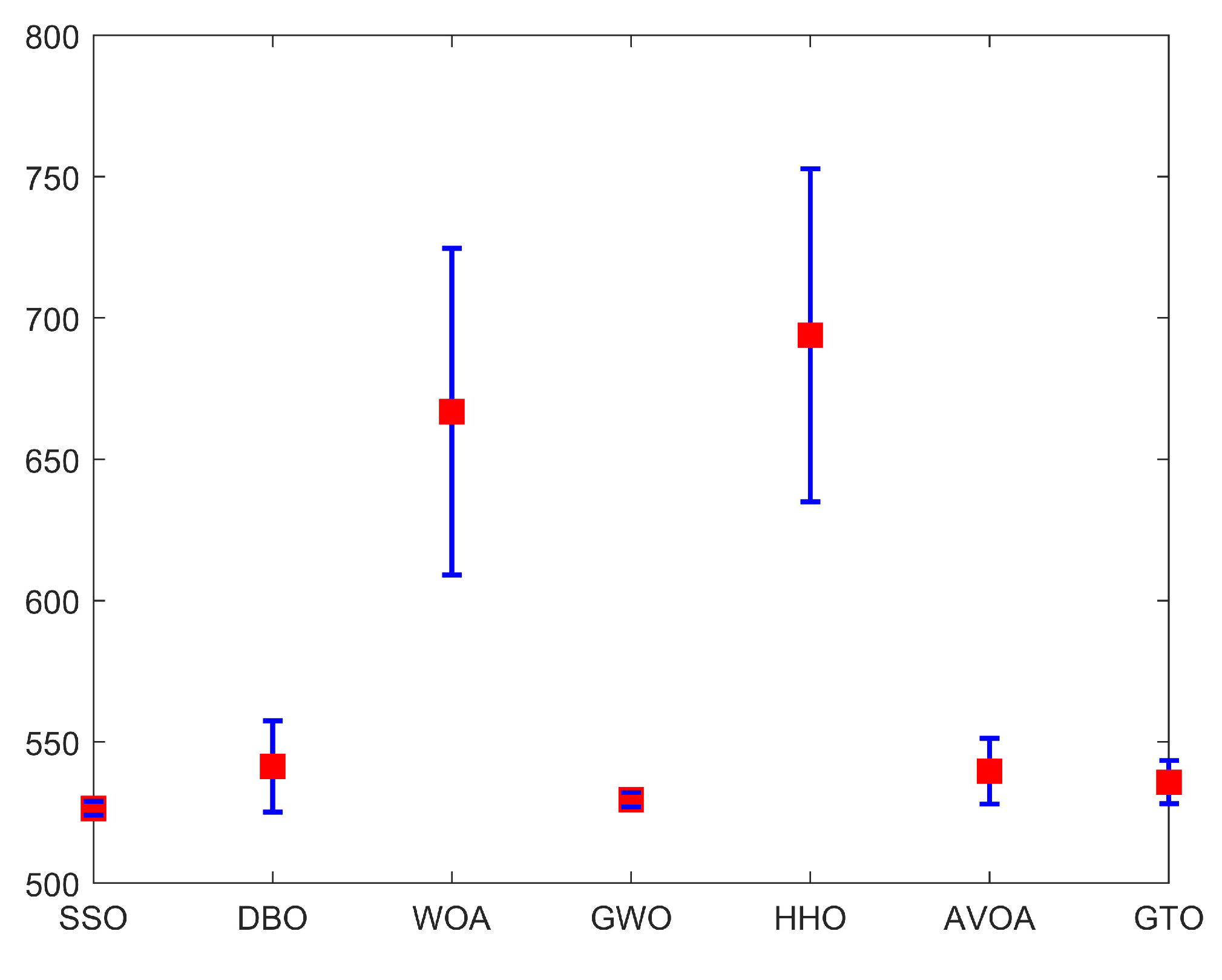
| Mean | 5.265 × 10² | 5.414 × 10² | 6.669 × 10² | 5.295 × 10² | 6.939 × 10² | 5.396 × 10² | 5.357 × 10² |
| Std | 2.496 × 100 | 1.613 × 101 | 5.779 × 101 | 2.538 × 100 | 5.889 × 101 | 1.169 × 101 | 7.616 × 100 |
| Best | 5.248 × 10² | 5.248 × 10² | 5.532 × 10² | 5.251 × 10² | 5.908 × 10² | 5.270 × 10² | 5.264 × 10² |
| Worst | 5.327 × 10² | 5.909 × 10² | 7.907 × 10² | 5.324 × 10² | 8.123 × 10² | 5.918 × 10² | 5.563 × 10² |
| Rank | 1 | 5 | 6 | 2 | 7 | 4 | 3 |
Disclaimer/Publisher’s Note: The statements, opinions and data contained in all publications are solely those of the individual author(s) and contributor(s) and not of MDPI and/or the editor(s). MDPI and/or the editor(s) disclaim responsibility for any injury to people or property resulting from any ideas, methods, instructions or products referred to in the content. |
© 2024 by the authors. Licensee MDPI, Basel, Switzerland. This article is an open access article distributed under the terms and conditions of the Creative Commons Attribution (CC BY) license (https://creativecommons.org/licenses/by/4.0/).
Share and Cite
Guo, J.; Yan, Z.; Sato, Y.; Zuo, Q. Salmon Salar Optimization: A Novel Natural Inspired Metaheuristic Method for Deep-Sea Probe Design for Unconventional Subsea Oil Wells. J. Mar. Sci. Eng. 2024, 12, 1802. https://doi.org/10.3390/jmse12101802
Guo J, Yan Z, Sato Y, Zuo Q. Salmon Salar Optimization: A Novel Natural Inspired Metaheuristic Method for Deep-Sea Probe Design for Unconventional Subsea Oil Wells. Journal of Marine Science and Engineering. 2024; 12(10):1802. https://doi.org/10.3390/jmse12101802
Chicago/Turabian StyleGuo, Jia, Zhou Yan, Yuji Sato, and Qiankun Zuo. 2024. "Salmon Salar Optimization: A Novel Natural Inspired Metaheuristic Method for Deep-Sea Probe Design for Unconventional Subsea Oil Wells" Journal of Marine Science and Engineering 12, no. 10: 1802. https://doi.org/10.3390/jmse12101802
APA StyleGuo, J., Yan, Z., Sato, Y., & Zuo, Q. (2024). Salmon Salar Optimization: A Novel Natural Inspired Metaheuristic Method for Deep-Sea Probe Design for Unconventional Subsea Oil Wells. Journal of Marine Science and Engineering, 12(10), 1802. https://doi.org/10.3390/jmse12101802