
Disturbance Observer-Based Model Predictive Control for an Unmanned Underwater Vehicle


Abstract
1. Introduction
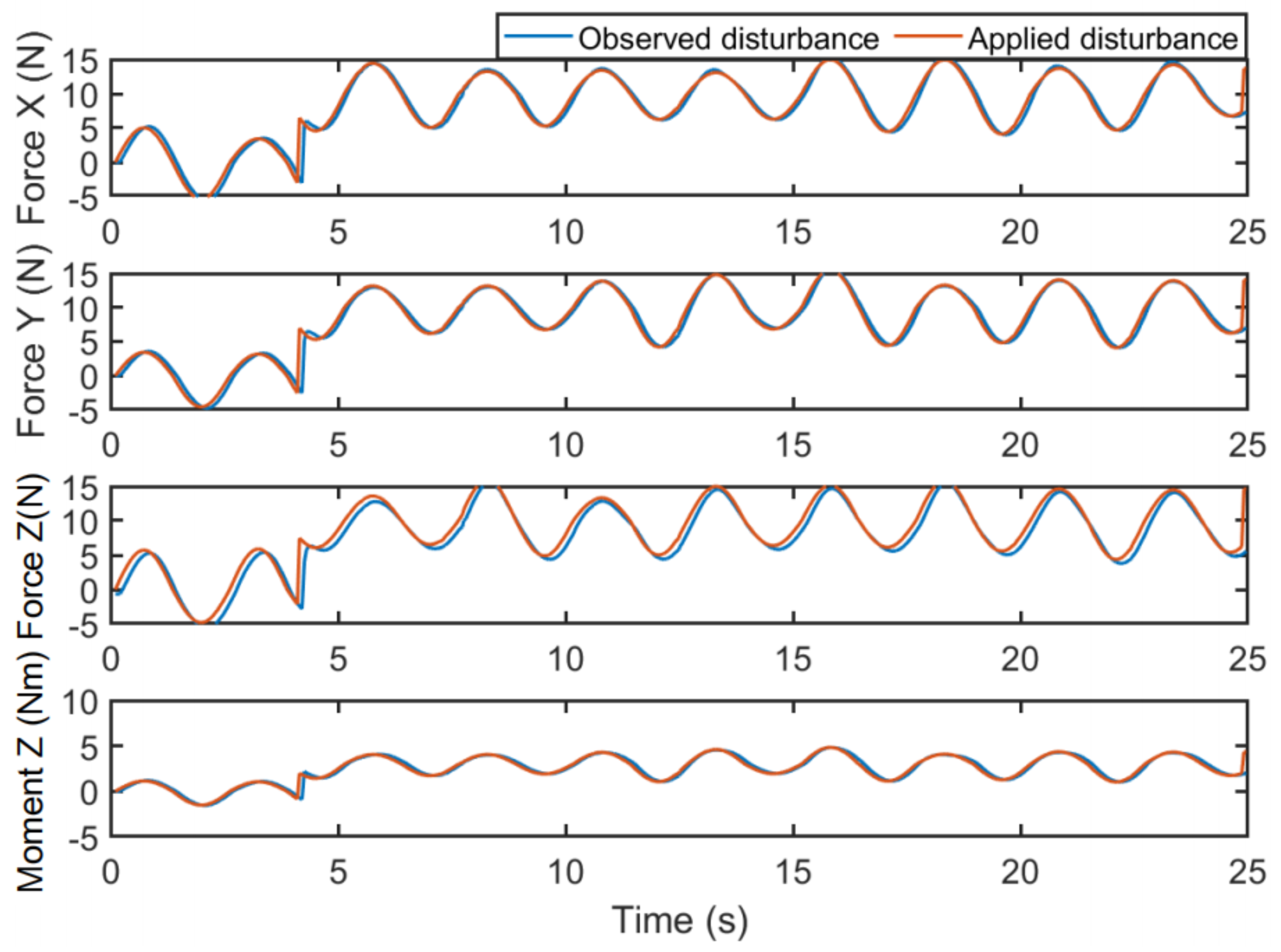
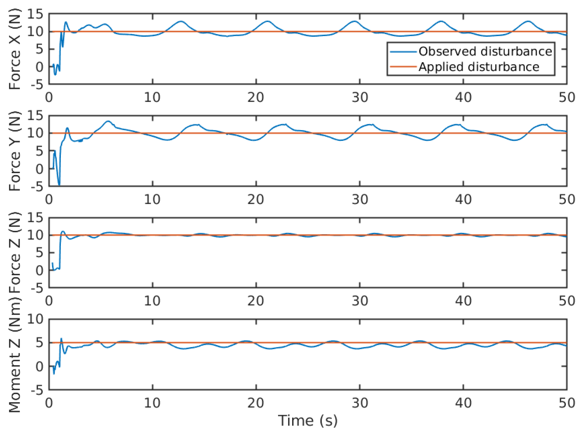
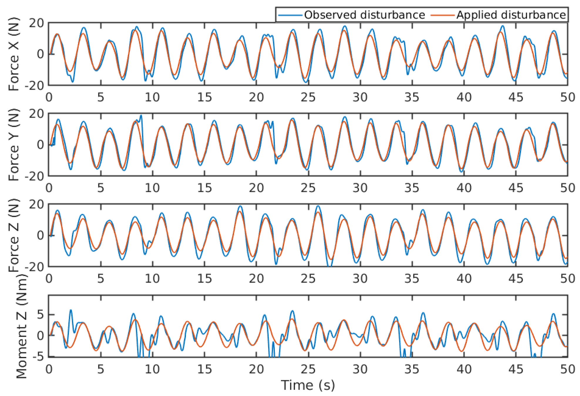
- The proposed EAOB demonstrates the capacity to effectively estimate disturbances in the presence of measurement noise. This is a notable improvement compared to previous literature, where the assumption of no measurement noise was prevalent, with only a limited number of papers addressing this crucial aspect.
- The proposed approach represents a significant advancement in compensating for disturbances by integrating real-time disturbance estimation into the prediction model of the MPC at each time step. This results in a parameter-varying model, surpassing previous methods that simply added estimated disturbances to the baseline control input. By employing this enhanced approach, more precise and adaptive control can be achieved, marking a notable improvement over previous compensation methods.
- In this work, the estimated disturbances are explicitly taken into account within the prediction horizon of the MPC framework. This enables the generation of optimal control inputs that effectively reject disturbances, surpassing previous related works that may not have explicitly considered disturbances within the optimization process. By incorporating the estimated disturbances throughout the MPC’s prediction horizon, this approach ensures the provision of control actions that account for the presence of disturbances.
2. Problem Formulation
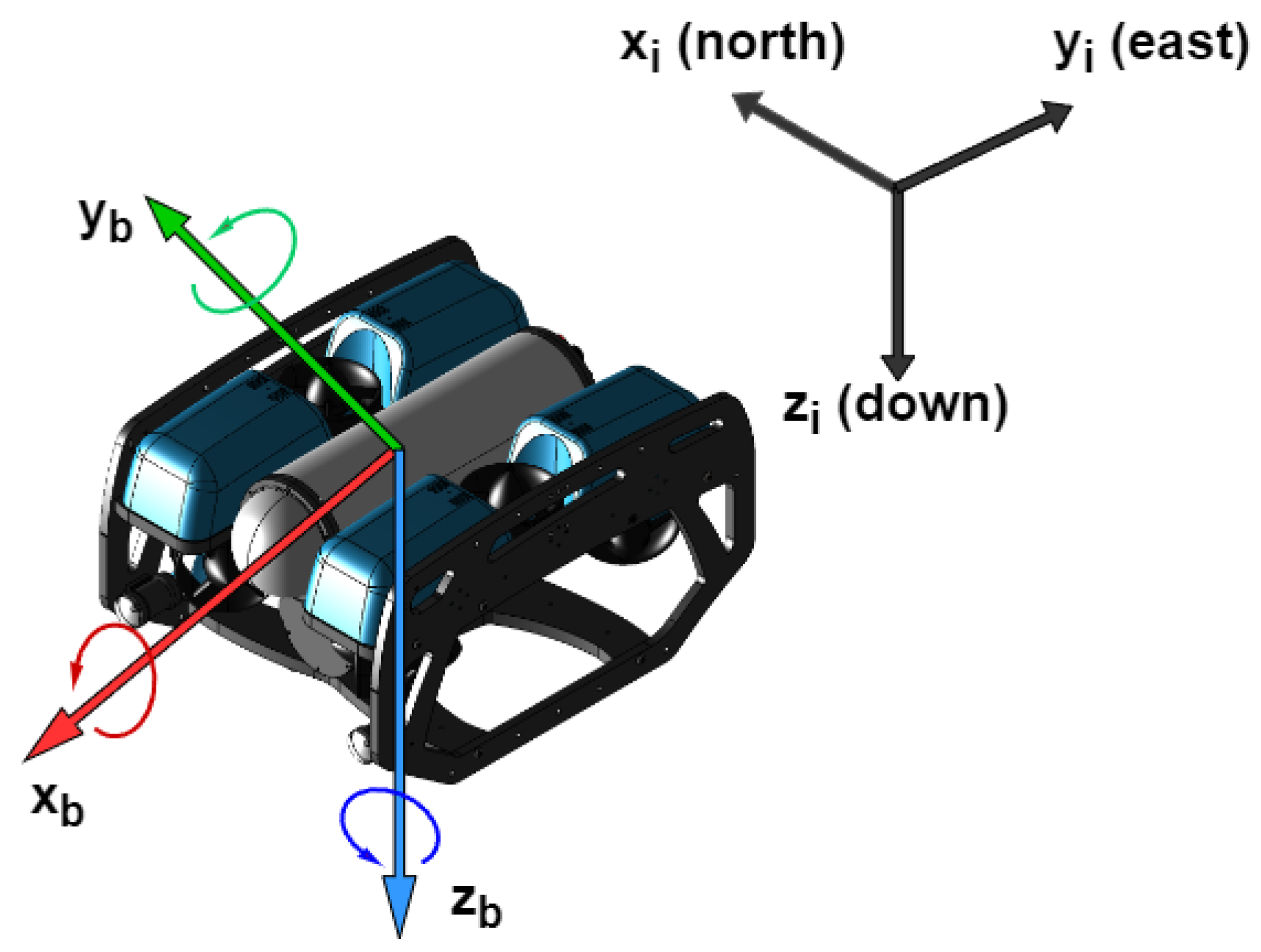
2.1. Kinematic Model
2.2. Kinetic Model
2.2.1. Rigid-Body Dynamics
2.2.2. Hydrodynamics
2.2.3. Hydrostatics
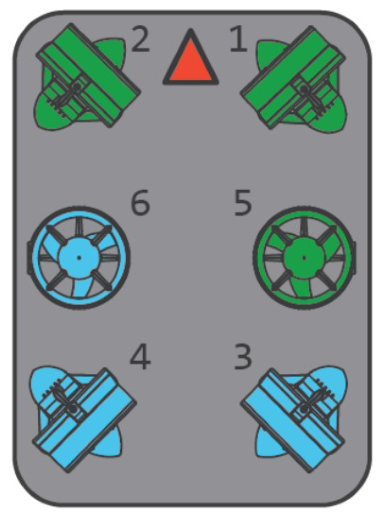
2.2.4. Propeller Model and Control Allocation
2.2.5. Nonlinear Model
3. Extended Active Observer
3.1. Observer Design
3.2. Stability Analysis
- 1.
- ,
- 2.
- .
- 3.
- Then the following is true:where in Equation (34) is bounded based on Assumption 1, and are positive constants.
- 1.
- uniformly completely observable;
- 2.
- uniformly completely controllable;
- 3.
- ;
- 4.
- /;
- 5.
- .
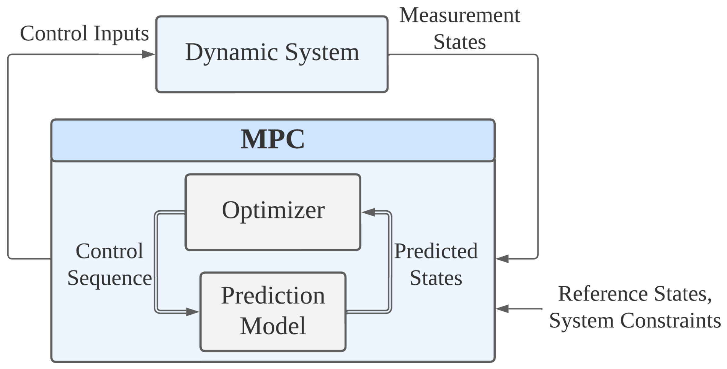
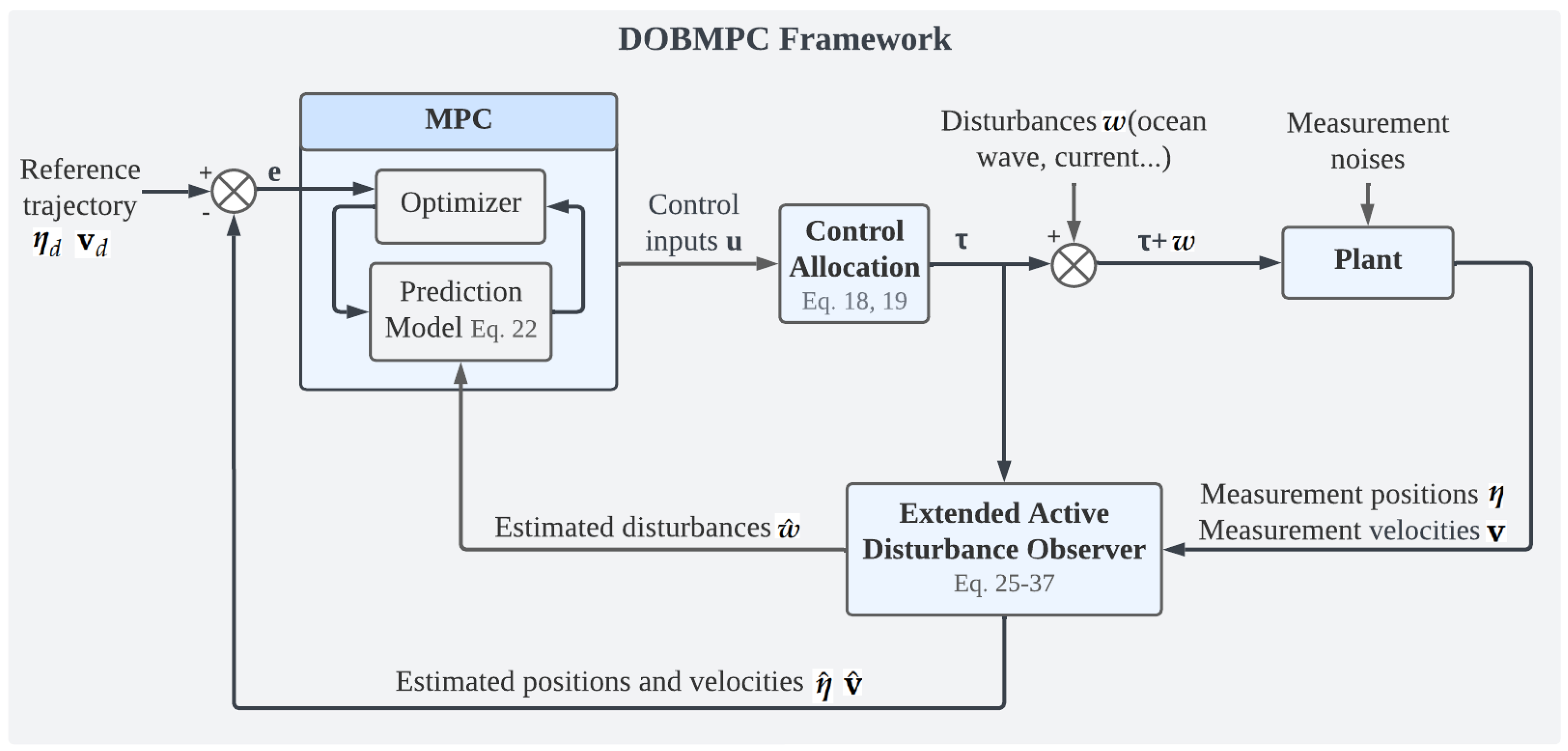
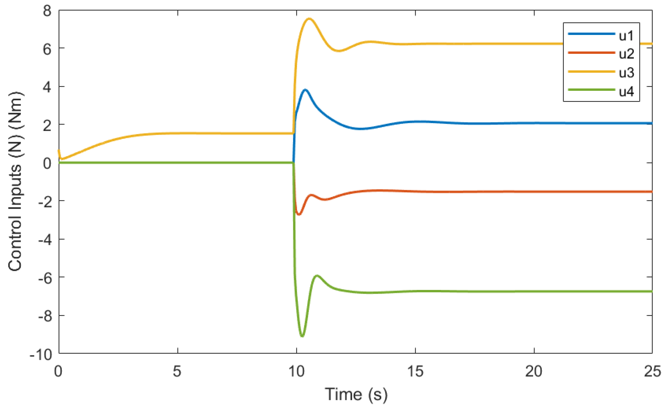
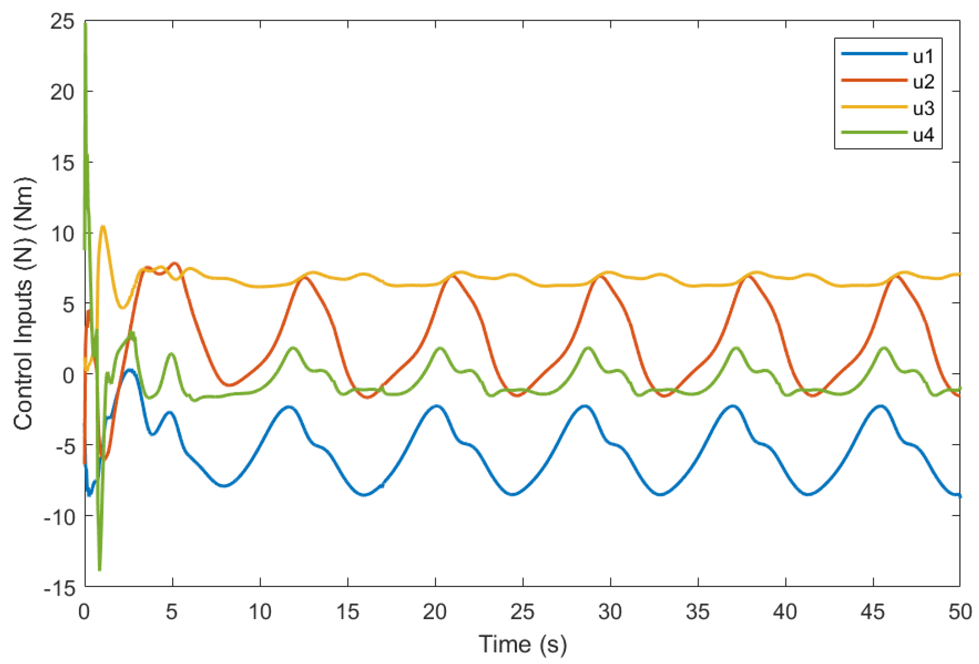
4. Disturbance Observer-Based Model Predictive Control (DOBMPC)
- Update the parameters within the disturbance term in the prediction model of the MPC, as represented by Equation (22), at the current time instant and within the prediction horizon , by incorporating the estimated disturbance obtained in the initial step.
- The OCP in the Equation (44) is solved to obtain the optimized control sequence .
- The first set of the control sequence is implemented in the dynamic system, while the rest will be treated as initial conditions in the next iteration.
- At the next sampling instant, the OCP in the Equation (44) will be solved again with the measurement states and new initial condition.
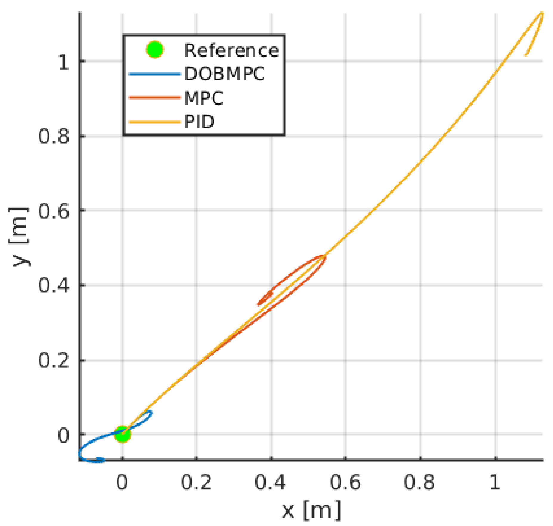
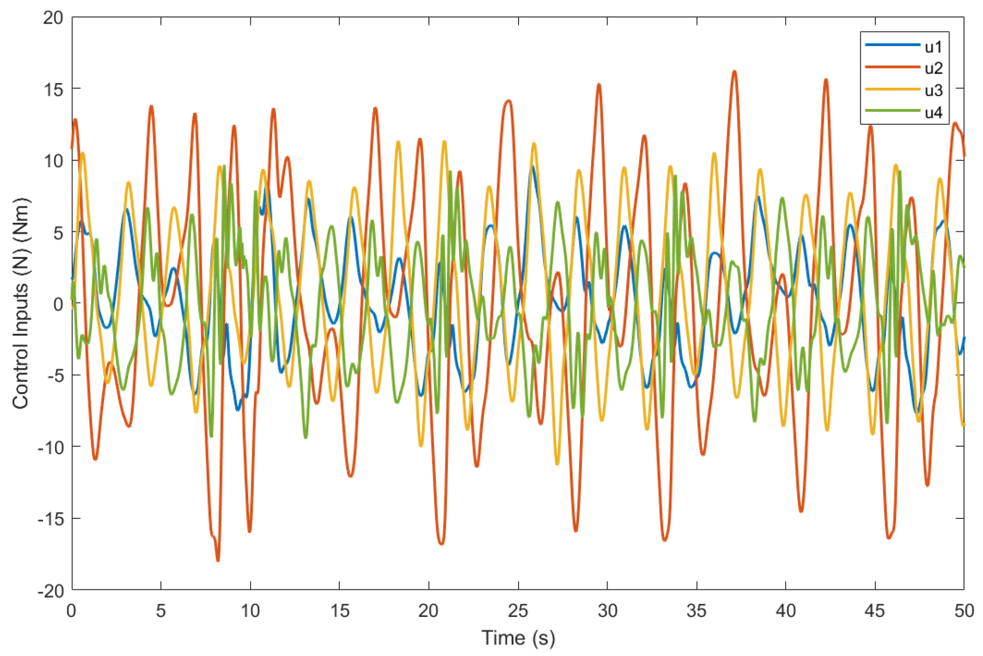
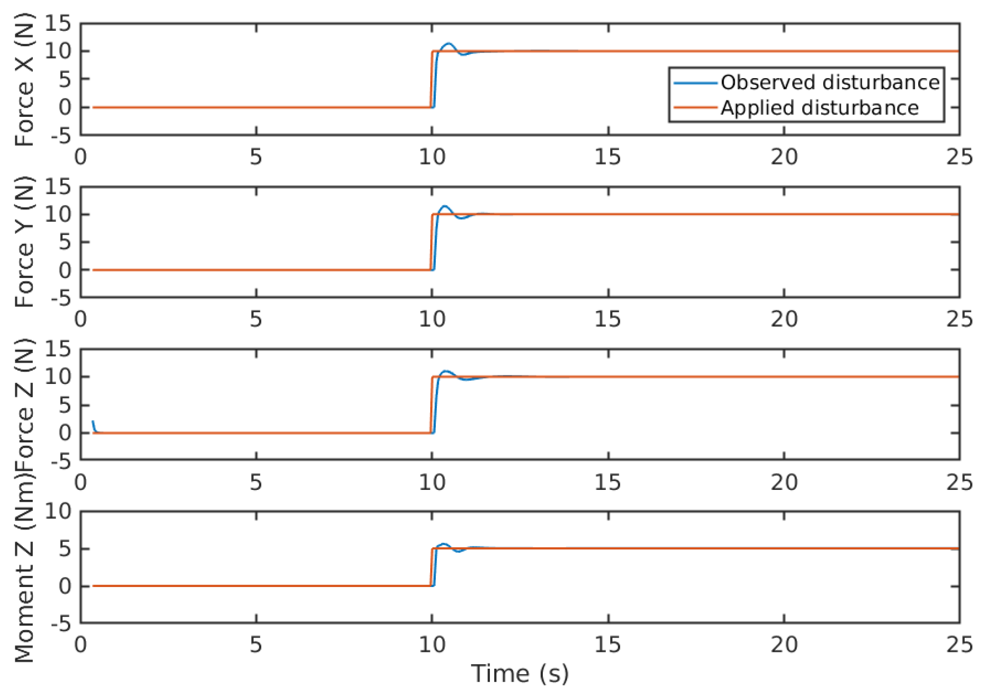
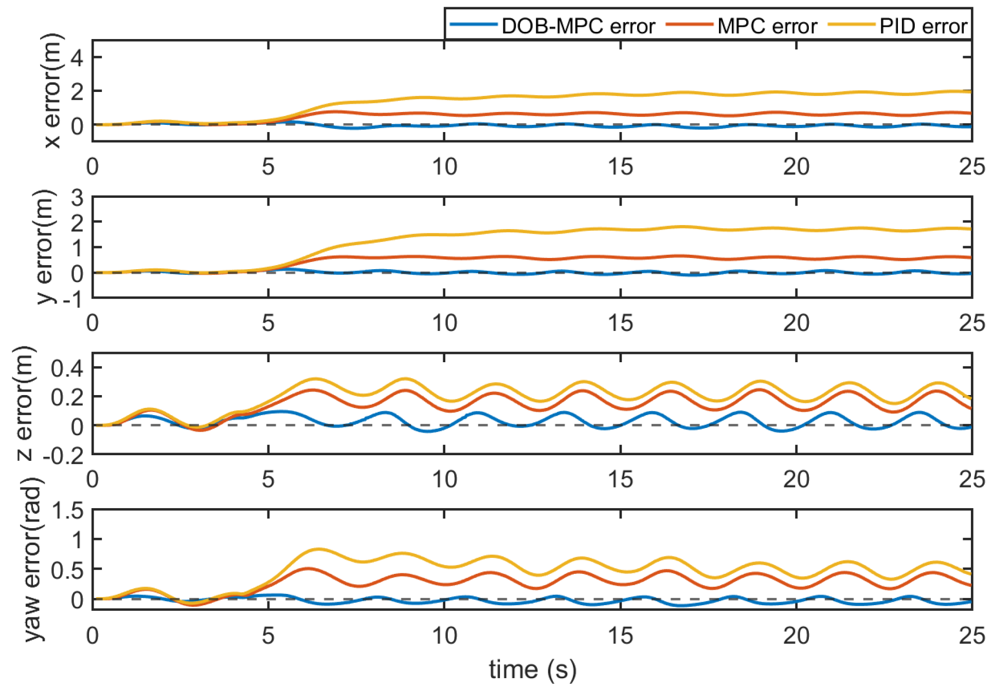
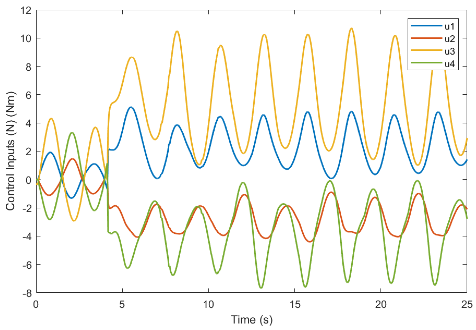
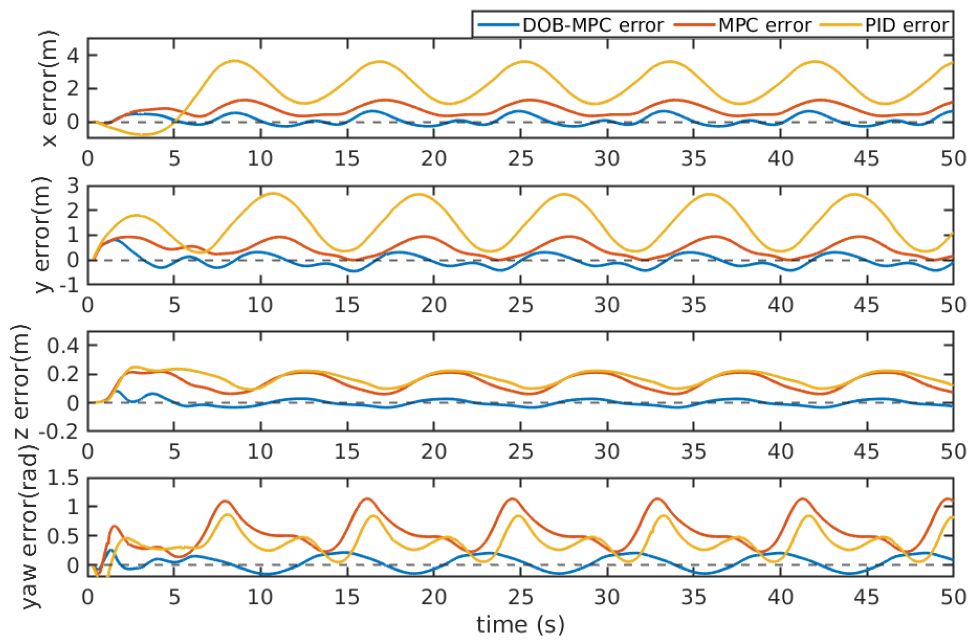
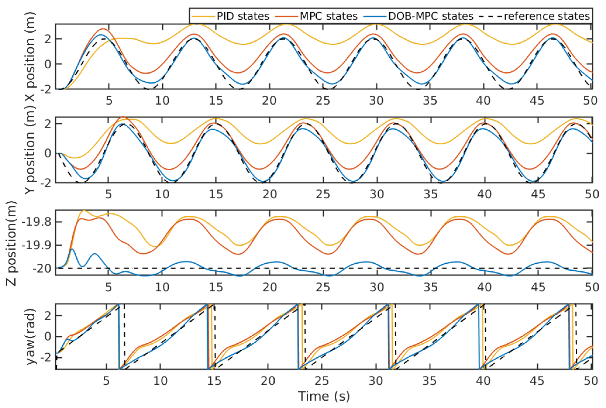
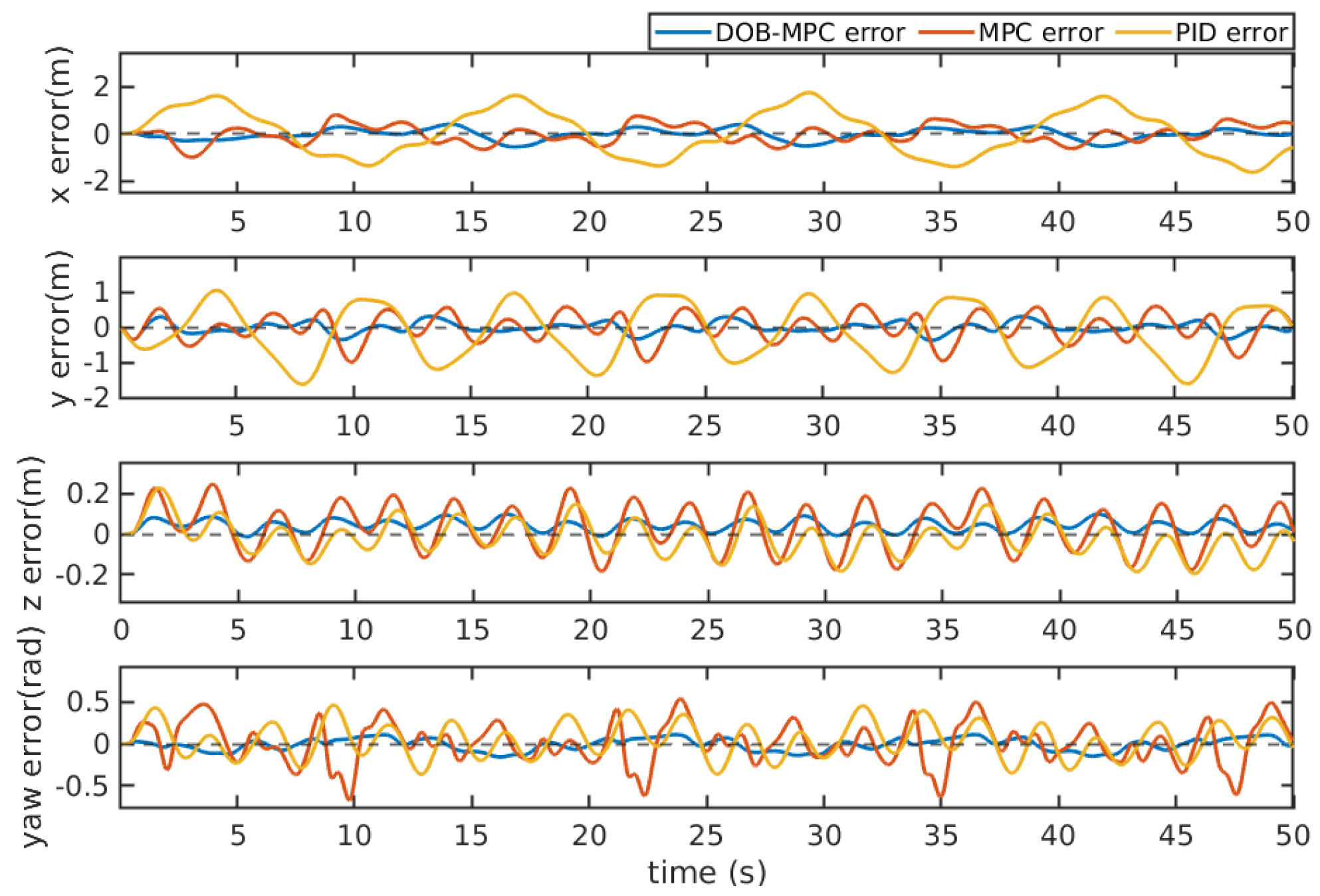
5. Results and Discussion
5.1. Dynamic Positioning Results
5.2. Trajectory Tracking Results
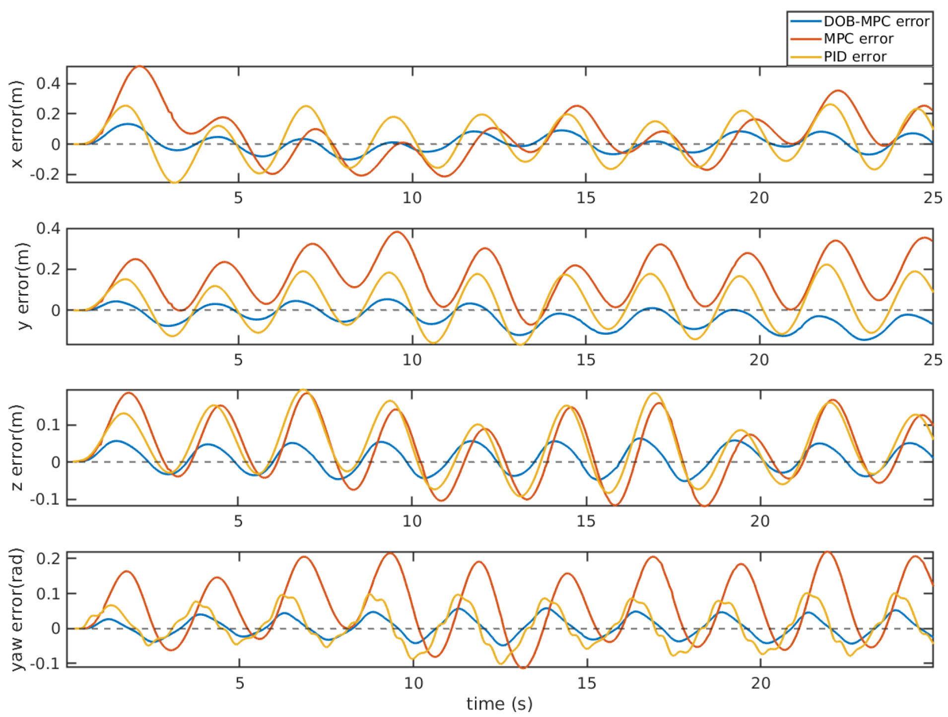
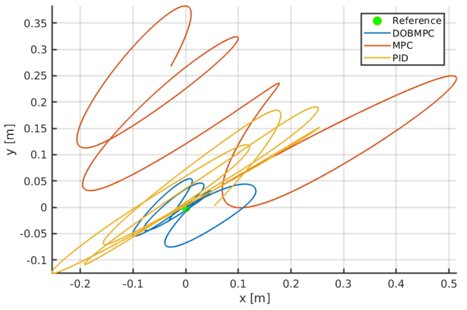
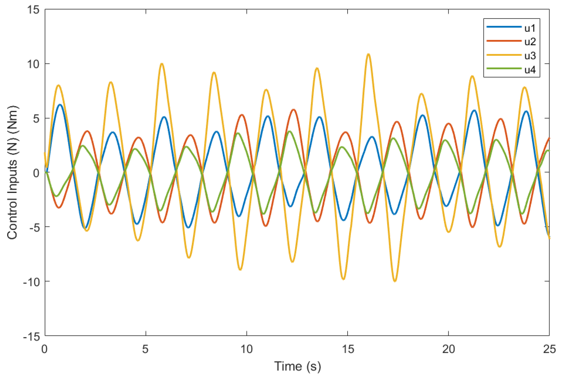
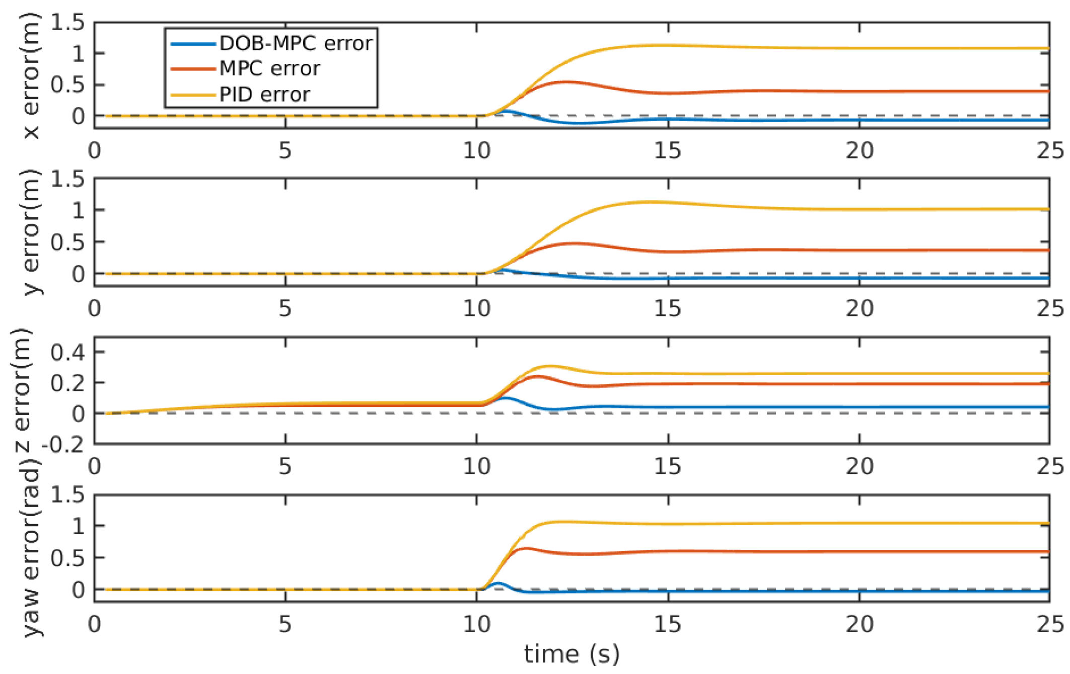
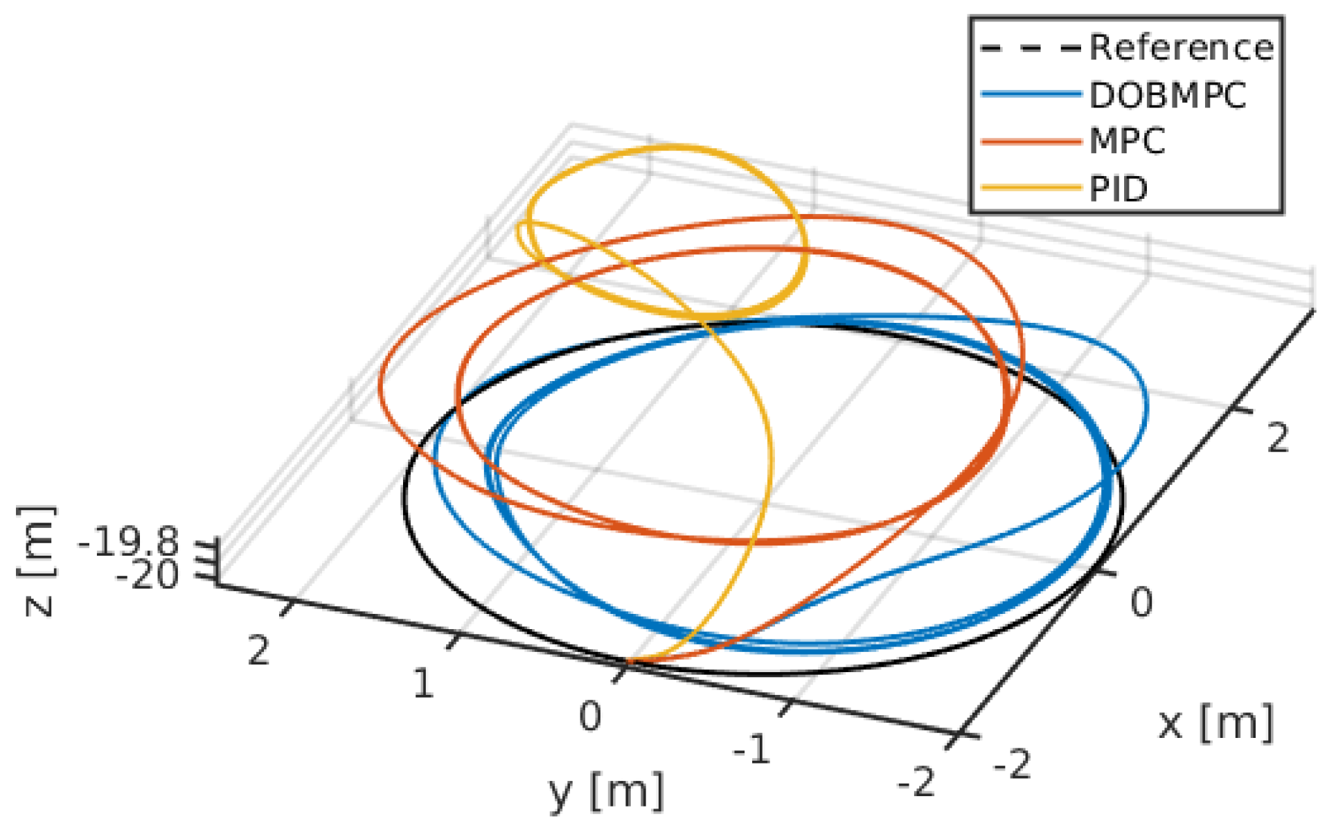
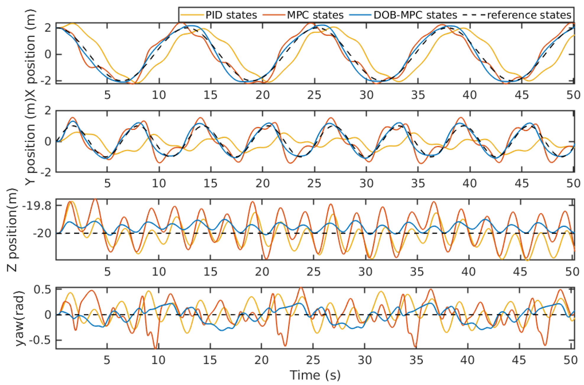
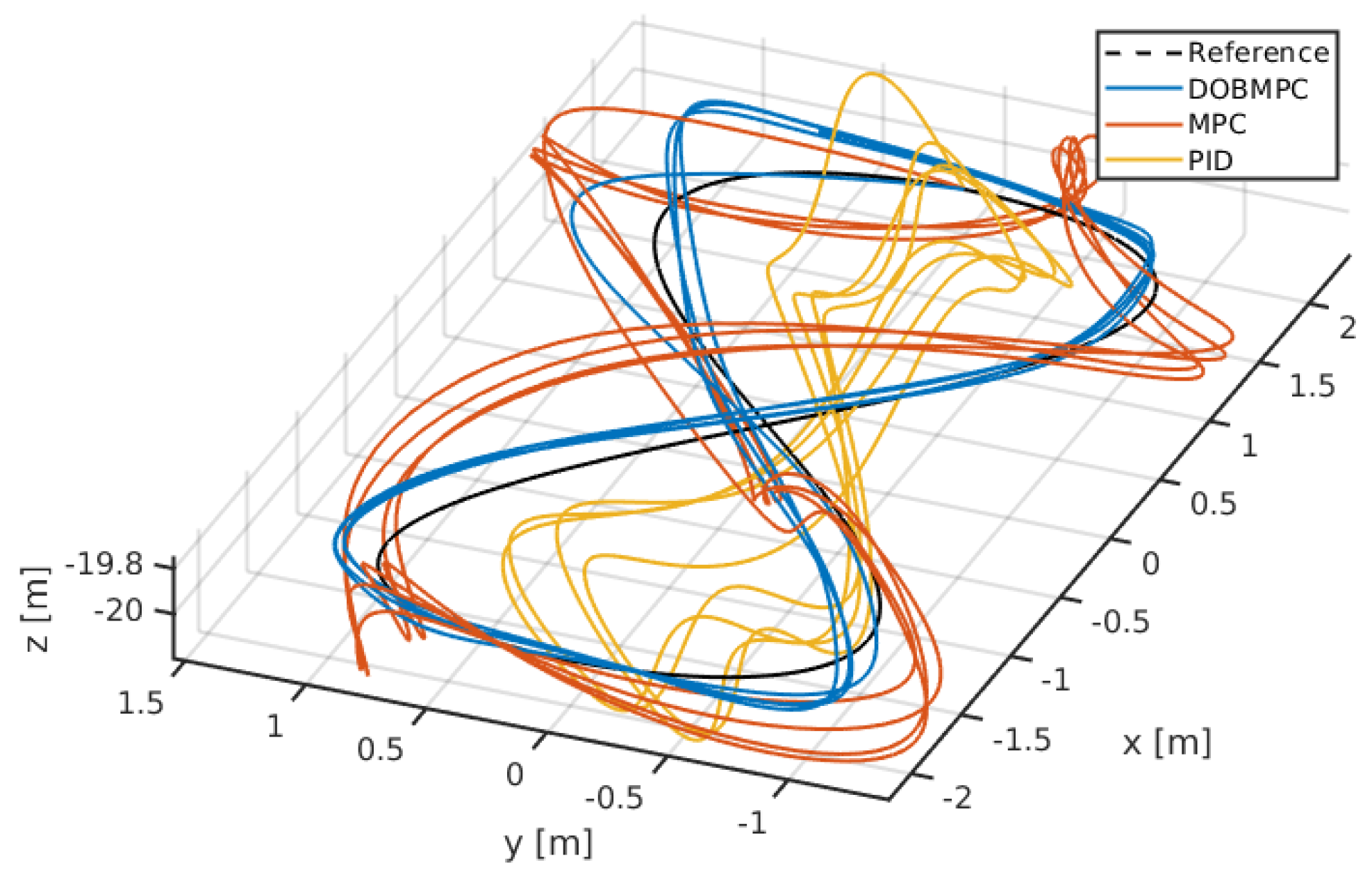
5.3. Results Analysis
6. Conclusions
Author Contributions
Funding
Institutional Review Board Statement
Informed Consent Statement
Data Availability Statement
Conflicts of Interest
References
- Hou, S.; Jiao, D.; Dong, B.; Wang, H.; Wu, G. Underwater inspection of bridge substructures using sonar and deep convolutional network. Adv. Eng. Inform. 2022, 52, 101545. [Google Scholar] [CrossRef]
- Hu, S.; Feng, R.; Wang, Z.; Zhu, C.; Wang, Z.; Chen, Y.; Huang, H. Control system of the autonomous underwater helicopter for pipeline inspection. Ocean. Eng. 2022, 266, 113190. [Google Scholar] [CrossRef]
- Barker, L.D.; Jakuba, M.V.; Bowen, A.D.; German, C.R.; Maksym, T.; Mayer, L.; Boetius, A.; Dutrieux, P.; Whitcomb, L.L. Scientific challenges and present capabilities in underwater robotic vehicle design and navigation for oceanographic exploration under-ice. Remote Sens. 2020, 12, 2588. [Google Scholar] [CrossRef]
- Mogstad, A.A.; Ødegård, Ø.; Nornes, S.M.; Ludvigsen, M.; Johnsen, G.; Sørensen, A.J.; Berge, J. Mapping the historical shipwreck figaro in the high arctic using underwater sensor-carrying robots. Remote Sens. 2020, 12, 997. [Google Scholar] [CrossRef]
- Summers, N.; Johnsen, G.; Mogstad, A.; Løvås, H.; Fragoso, G.; Berge, J. Underwater hyperspectral imaging of Arctic macroalgal habitats during the polar night using a novel mini-ROV-UHI portable system. Remote Sens. 2022, 14, 1325. [Google Scholar] [CrossRef]
- Preuß, H.; Cherewko, V.; Wollstadt, J.; Wendt, A.; Renkewitz, H. Crawfish Goes Swimming: Hardware Architecture of a Crawling Skid for Underwater Maintenance with a BlueROV2. In Proceedings of the OCEANS 2022, Hampton Roads, VA, USA, 17–20 October 2022; pp. 1–5. [Google Scholar] [CrossRef]
- Mai, C.; Benzon, M.V.; Sørensen, F.F.; Klemmensen, S.S.; Pedersen, S.; Liniger, J. Design of an Autonomous ROV for Marine Growth Inspection and Cleaning. In Proceedings of the 2022 IEEE/OES Autonomous Underwater Vehicles Symposium (AUV), Singapore, 19–21 September 2022; pp. 1–6. [Google Scholar] [CrossRef]
- Mao, J.; Song, G.; Hao, S.; Zhang, M.; Song, A. Development of a Lightweight Underwater Manipulator for Delicate Structural Repair Operations. IEEE Robot. Autom. Lett. 2023, 8, 6563–6570. [Google Scholar] [CrossRef]
- Woolsey, C. Review of Marine Control Systems: Guidance, Navigation, and Control of Ships, Rigs and Underwater Vehicles. J. Guid. Control. Dyn. 2005, 28, 574–575. [Google Scholar] [CrossRef]
- Liu, L.; Zhang, L.; Pan, G.; Zhang, S. Robust yaw control of autonomous underwater vehicle based on fractional-order PID controller. Ocean. Eng. 2022, 257, 111493. [Google Scholar] [CrossRef]
- Hasan, M.W.; Abbas, N.H. Disturbance Rejection for Underwater robotic vehicle based on adaptive fuzzy with nonlinear PID controller. ISA Trans. 2022, 130, 360–376. [Google Scholar] [CrossRef]
- Bingul, Z.; Gul, K. Intelligent-PID with PD Feedforward Trajectory Tracking Control of an Autonomous Underwater Vehicle. Machines 2023, 11, 300. [Google Scholar] [CrossRef]
- Healey, A.; Lienard, D. Multivariable sliding mode control for autonomous diving and steering of unmanned underwater vehicles. IEEE J. Ocean. Eng. 1993, 18, 327–339. [Google Scholar] [CrossRef]
- Yan, Z.; Wang, M.; Xu, J. Robust adaptive sliding mode control of underactuated autonomous underwater vehicles with uncertain dynamics. Ocean. Eng. 2019, 173, 802–809. [Google Scholar] [CrossRef]
- Lv, T.; Zhou, J.; Wang, Y.; Gong, W.; Zhang, M. Sliding mode based fault tolerant control for autonomous underwater vehicle. Ocean. Eng. 2020, 216, 107855. [Google Scholar] [CrossRef]
- Carreras, M.; Batlle, J.; Ridao, P. Hybrid coordination of reinforcement learning-based behaviors for AUV control. In Proceedings of the 2001 IEEE/RSJ International Conference on Intelligent Robots and Systems. Expanding the Societal Role of Robotics in the the Next Millennium (Cat. No.01CH37180), Maui, HI, USA, 29 October–3 November 2001; Volume 3, pp. 1410–1415. [Google Scholar] [CrossRef]
- Elhaki, O.; Shojaei, K. A robust neural network approximation-based prescribed performance output-feedback controller for autonomous underwater vehicles with actuators saturation. Eng. Appl. Artif. Intell. 2020, 88, 103382. [Google Scholar] [CrossRef]
- Patre, B.M.; Londhe, P.S.; Waghmare, L.M.; Mohan, S. Disturbance estimator based non-singular fast fuzzy terminal sliding mode control of an autonomous underwater vehicle. Ocean. Eng. 2018, 159, 372–387. [Google Scholar] [CrossRef]
- Lakhekar, G.V.; Waghmare, L.M.; Roy, R.G. Disturbance Observer-Based Fuzzy Adapted S-Surface Controller for Spatial Trajectory Tracking of Autonomous Underwater Vehicle. IEEE Trans. Intell. Veh. 2019, 4, 622–636. [Google Scholar] [CrossRef]
- Dai, Y.; Wu, D.; Yu, S.; Yan, Y. Robust control of underwater vehicle-manipulator system using grey wolf optimizer-based nonlinear disturbance observer and H-infinity controller. Complexity 2020, 2020, 6549572. [Google Scholar] [CrossRef]
- Guerrero, J.; Torres, J.; Creuze, V.; Chemori, A. Adaptive disturbance observer for trajectory tracking control of underwater vehicles. Ocean. Eng. 2020, 200, 107080. [Google Scholar] [CrossRef]
- Kamel, M.; Stastny, T.; Alexis, K.; Siegwart, R. Model predictive control for trajectory tracking of unmanned aerial vehicles using robot operating system. In Robot Operating System (ROS) the Complete Reference (Volume 2); Springer: Cham, Switzerland, 2017; pp. 3–39. [Google Scholar] [CrossRef]
- Veksler, A.; Johansen, T.A.; Borrelli, F.; Realfsen, B. Dynamic Positioning With Model Predictive Control. IEEE Trans. Control Syst. Technol. 2016, 24, 1340–1353. [Google Scholar] [CrossRef]
- Medagoda, L.; Williams, S.B. Model predictive control of an autonomous underwater vehicle in an in situ estimated water current profile. In Proceedings of the 2012 Oceans, Yeosu, Republic of Korea, 21–24 May 2012; pp. 1–8. [Google Scholar] [CrossRef]
- Shen, C.; Shi, Y.; Buckham, B. Trajectory Tracking Control of an Autonomous Underwater Vehicle Using Lyapunov-Based Model Predictive Control. IEEE Trans. Ind. Electron. 2018, 65, 5796–5805. [Google Scholar] [CrossRef]
- Cao, Y.; Li, B.; Li, Q.; Stokes, A.A.; Ingram, D.M.; Kiprakis, A. A Nonlinear Model Predictive Controller for Remotely Operated Underwater Vehicles With Disturbance Rejection. IEEE Access 2020, 8, 158622–158634. [Google Scholar] [CrossRef]
- Arcos-Legarda, J.; Gutiérrez, Á. Robust Model Predictive Control Based on Active Disturbance Rejection Control for a Robotic Autonomous Underwater Vehicle. J. Mar. Sci. Eng. 2023, 11, 929. [Google Scholar] [CrossRef]
- Robotics, B. BlueROV2: The World’s Most Affordable High-Performance ROV; BlueROV2 Datasheet; Blue Robotics: Torrance, CA, USA, 2016. [Google Scholar]
- Fossen, T.I. Handbook of Marine Craft Hydrodynamics and Motion Control; John Wiley & Sons: Hoboken, NJ, USA, 2011; pp. 167–183. [Google Scholar]
- Kane, T.R.; Likins, P.W.; Levinson, D.A. Spacecraft Dynamics; McGraw-Hill Book Company: New York, NY, USA, 1983. [Google Scholar]
- Chondros, T.G. Distinguished Figures in Mechanism and Machine Science: Their Contributions and Legacies Part 1; Springer: Berlin/Heidelberg, Germany, 2007; pp. 1–30. [Google Scholar]
- von Benzon, M.; Sørensen, F.F.; Uth, E.; Jouffroy, J.; Liniger, J.; Pedersen, S. An Open-Source Benchmark Simulator: Control of a BlueROV2 Underwater Robot. J. Mar. Sci. Eng. 2022, 10, 1898. [Google Scholar] [CrossRef]
- Alfian, R.I.; Ma’arif, A.; Sunardi, S. Noise reduction in the accelerometer and gyroscope sensor with the Kalman filter algorithm. J. Robot. Control 2021, 2, 180–189. [Google Scholar] [CrossRef]
- Bai, Y.; Wang, X.; Jin, X.; Su, T.; Kong, J.; Zhang, B. Adaptive filtering for MEMS gyroscope with dynamic noise model. ISA Trans. 2020, 101, 430–441. [Google Scholar] [CrossRef] [PubMed]
- Frogerais, P.; Bellanger, J.J.; Senhadji, L. Various ways to compute the continuous-discrete extended Kalman filter. IEEE Trans. Autom. Control 2011, 57, 1000–1004. [Google Scholar] [CrossRef]
- Butcher, J.C. A history of Runge-Kutta methods. Appl. Numer. Math. 1996, 20, 247–260. [Google Scholar] [CrossRef]
- Chan, L.; Naghdy, F.; Stirling, D. Extended active observer for force estimation and disturbance rejection of robotic manipulators. Robot. Auton. Syst. 2013, 61, 1277–1287. [Google Scholar] [CrossRef]
- Kalman, R.E.; Bucy, R.S. New results in linear filtering and prediction theory. J. Fluids Eng. 1961, 84, 95–108. [Google Scholar] [CrossRef]
- Diehl, M.; Bock, H.G.; Diedam, H.; Wieber, P.B. Fast direct multiple shooting algorithms for optimal robot control. In Fast Motions in Biomechanics and Robotics: Optimization and Feedback Control; Springer: Berlin/Heidelberg, Germany, 2006; pp. 65–93. [Google Scholar] [CrossRef]
- Verschueren, R.; Frison, G.; Kouzoupis, D.; van Duijkeren, N.; Zanelli, A.; Quirynen, R.; Diehl, M. Towards a modular software package for embedded optimization. IFAC-PapersOnLine 2018, 51, 374–380. [Google Scholar] [CrossRef]
- Feller, C.; Ebenbauer, C. Sparsity-exploiting anytime algorithms for model predictive control: A relaxed barrier approach. IEEE Trans. Control Syst. Technol. 2020, 28, 425–435. [Google Scholar] [CrossRef]
- Gharbi, M.; Ebenbauer, C. Anytime MHE-based output feedback MPC. IFAC-PapersOnLine 2021, 54, 264–271. [Google Scholar] [CrossRef]
- Hosseinzadeh, M.; Sinopoli, B.; Kolmanovsky, I.; Baruah, S. Robust to early termination model predictive control. IEEE Trans. Autom. Control 2023. early access. [Google Scholar] [CrossRef]
- Manhães, M.M.M.; Scherer, S.A.; Voss, M.; Douat, L.R.; Rauschenbach, T. UUV Simulator: A Gazebo-based package for underwater intervention and multi-robot simulation. In Proceedings of the OCEANS 2016 MTS/IEEE, Monterey, CA, USA, 19–23 September 2016. [Google Scholar] [CrossRef]
- Hasselmann, K.; Barnett, T.P.; Bouws, E.; Carlson, H.; Cartwright, D.E.; Enke, K.; Ewing, J.; Gienapp, A.; Hasselmann, D.; Kruseman, P.; et al. Measurements of wind-wave growth and swell decay during the Joint North Sea Wave Project (JONSWAP). In Ergaenzungsheft zur Deutschen Hydrographischen Zeitschrift, Reihe A; Deutsches Hydrographisches Institut: Hamburg, Germany, 1973; pp. 1–95. [Google Scholar]
- Ohhira, T.; Kawamura, A.; Shimada, A.; Murakami, T. An underwater quadrotor control with wave-disturbance compensation by a UKF. IFAC-PapersOnLine 2020, 53, 9017–9022. [Google Scholar] [CrossRef]
- Ullah, B.; Ovinis, M.; Baharom, M.B.; Ali, S.S.A.; Khan, B.; Javaid, M.Y. Effect of waves and current on motion control of underwater gliders. J. Mar. Sci. Technol. 2020, 25, 549–562. [Google Scholar] [CrossRef]
- Marechal, G.; Ardhuin, F. Surface Currents and Significant Wave Height Gradients: Matching Numerical Models and High-Resolution Altimeter Wave Heights in the Agulhas Current Region. J. Geophys. Res. Ocean. 2021, 126, e2020JC016564. [Google Scholar] [CrossRef]
- Li, Z.; Deng, G.; Queutey, P.; Bouscasse, B.; Ducrozet, G.; Gentaz, L.; Le Touzé, D.; Ferrant, P. Comparison of wave modeling methods in CFD solvers for ocean engineering applications. Ocean. Eng. 2019, 188, 106237. [Google Scholar] [CrossRef]


| Surge Sway Heave | Roll Pitch Yaw | |
|---|---|---|
| Position | x y z (m) | (rad) |
| Velocity | u v w (m/s) | p q r (rad/s) |
| Forces and Moments | X Y Z (N) | K M N (Nm) |
| Control Inputs | (N) | / / (Nm) |
| Disturbances | (N) | (Nm) |
| Measured Disturbances | (N) | / / (Nm) |
| Unmeasured Disturbances | / / / | / (Nm) |
| Added Mass | (kg) | (kgm2/rad) |
| Linear Damping | (Ns/m) | (Ns/rad) |
| Nonlinear Damping | (Ns2/m2) | (Ns2/rad2) |
| Feedback Variables | x y z (m) | (rad) |
| u v w (m/s) | p q r (rad/s) | |
| X Y Z (N) | / / (Nm) |
| Parameter | Value |
|---|---|
| m | 11.26 kg |
| W | 112.8 N |
| B | 114.8 N |
| 0.3 kgm2 | |
| 0.63 kgm2 | |
| 0.58 kgm2 |
| Direction | Parameter | Value |
|---|---|---|
| Surge | 1.7182 kg | |
| Sway | 0 kg | |
| Heave | 5.468 kg | |
| Roll | 0 kgm2/rad | |
| Pitch | 1.2481 kgm2/rad | |
| Yaw | 0.4006 kgm2/rad | |
| Surge | −11.7391 Ns/m | |
| Sway | −20 Ns/m | |
| Heave | −31.8678 Ns/m | |
| Roll | −25 Ns/rad | |
| Pitch | −44.9085 Ns/rad | |
| Yaw | −5 Ns/rad |
| Controller Parameters | Value |
|---|---|
| Prediction horizon | 60 |
| Sample time (s) | 0.05 |
| Q | [300 300 150 10 10 150 10 10 10 10 10 10 15 15 15 0.5] |
| [300 300 150 10 10 150 10 10 10 10 10 10] | |
| OCP time (ms) | 7 |
| Control Gain | Surge | Sway | Heave | Yaw |
|---|---|---|---|---|
| 5 | 5 | 5 | 7 | |
| 0.05 | 0.05 | 0.05 | 0.1 | |
| 1.2 | 1.2 | 1.2 | 0.6 |
| Motion | Disturbance | Direction | PID (m) | MPC (m) | DOBMPC (m) |
|---|---|---|---|---|---|
| X | 0.1374 | 0.1689 | 0.0537 | ||
| Dynamic | Periodic | Y | 0.1095 | 0.1934 | 0.0605 |
| Positioning | wave effects | Z | 0.0871 | 0.0896 | 0.0350 |
| Yaw | 0.0536 | 0.1108 | 0.0282 | ||
| X | 0.7893 | 0.3099 | 0.0521 | ||
| Dynamic | Constant | Y | 0.7544 | 0.2882 | 0.0482 |
| Positioning | current effects | Z | 0.2032 | 0.1508 | 0.0469 |
| Yaw | 0.7858 | 0.4547 | 0.0491 | ||
| Superposition | X | 1.4991 | 0.5666 | 0.0932 | |
| Dynamic | of wave | Y | 1.3921 | 0.5151 | 0.0501 |
| Positioning | and currents | Z | 0.2179 | 0.1603 | 0.0486 |
| Yaw | 0.5141 | 0.3039 | 0.1100 | ||
| Circular | X | 2.3626 | 0.8012 | 0.2924 | |
| Trajectory | Constant | Y | 1.6433 | 0.5521 | 0.2629 |
| Tracking | current effects | Z | 0.1763 | 0.1510 | 0.0233 |
| Yaw | 0.4355 | 0.6325 | 0.2582 | ||
| Lemniscate | X | 0.9854 | 0.3764 | 0.2306 | |
| Trajectory | Constant | Y | 0.7732 | 0.3844 | 0.1504 |
| Tracking | current effects | Z | 0.0877 | 0.1133 | 0.0510 |
| Yaw | 0.2059 | 0.2413 | 0.1457 |
Disclaimer/Publisher’s Note: The statements, opinions and data contained in all publications are solely those of the individual author(s) and contributor(s) and not of MDPI and/or the editor(s). MDPI and/or the editor(s) disclaim responsibility for any injury to people or property resulting from any ideas, methods, instructions or products referred to in the content. |
© 2024 by the authors. Licensee MDPI, Basel, Switzerland. This article is an open access article distributed under the terms and conditions of the Creative Commons Attribution (CC BY) license (https://creativecommons.org/licenses/by/4.0/).
Share and Cite
Hu, Y.; Li, B.; Jiang, B.; Han, J.; Wen, C.-Y. Disturbance Observer-Based Model Predictive Control for an Unmanned Underwater Vehicle. J. Mar. Sci. Eng. 2024, 12, 94. https://doi.org/10.3390/jmse12010094
Hu Y, Li B, Jiang B, Han J, Wen C-Y. Disturbance Observer-Based Model Predictive Control for an Unmanned Underwater Vehicle. Journal of Marine Science and Engineering. 2024; 12(1):94. https://doi.org/10.3390/jmse12010094
Chicago/Turabian StyleHu, Yang, Boyang Li, Bailun Jiang, Jixuan Han, and Chih-Yung Wen. 2024. "Disturbance Observer-Based Model Predictive Control for an Unmanned Underwater Vehicle" Journal of Marine Science and Engineering 12, no. 1: 94. https://doi.org/10.3390/jmse12010094
APA StyleHu, Y., Li, B., Jiang, B., Han, J., & Wen, C.-Y. (2024). Disturbance Observer-Based Model Predictive Control for an Unmanned Underwater Vehicle. Journal of Marine Science and Engineering, 12(1), 94. https://doi.org/10.3390/jmse12010094