Tsunami Inundation Modelling in a Built-In Coastal Environment with Adaptive Mesh Refinement: The Onagawa Benchmark Test

Abstract

In tsunami studies, understanding the intricate dynamics in the swash area, characterised by the shoaling effect, remains a challenge. In this study, we employed the adaptive mesh refinement (AMR) method to model tsunami inundation and propagation in the Onagawa town physical flume experiment. Using the open-source flow solver Basilisk, we implemented the Saint-Venant (SV) equations, Serre–Green–Naghdi (SGN) equations, and a nonhydrostatic multilayer (ML) extension of the SGN equations. A hydraulic bore tsunami-like wave was used as the input boundary condition. The objective was to assess the efficiency of the AMR method with nonhydrostatic tsunami models in overcoming limitations in 2D and quasi-3D models in flume experiments, particularly with respect to improving accuracy in arrival time and run-up detection. The results indicate improved performance of the SGN and SV models in determining tsunami arrival times. The ML model demonstrated enhanced wave run-up simulations on complex built-in terrain. The refined roughness coefficient determined using the ML solver captured the arrival time well in the northern section of the Onagawa model, albeit with a 1 s delay. The AMR method offered a computationally stable solution with an 86.3% reduction in computational time compared to a constant grid. While effective, the nonhydrostatic models entail the use of a great deal of computational resources.

1. Introduction

The great Japanese earthquake on 11 March 2011 generated a significant tsunami that reached the northeastern coast, covering an extensive area of over 500 km². This disaster had profound consequences, claiming more than 15,000 lives and ranking as the second-largest human loss event after the 2004 Indian Ocean tsunami [1,2]. The economic toll was staggering, with estimated losses reaching approximately USD 210 billion, making it the costliest natural disaster on record [3].

In the aftermath of the 2011 Tohoku tsunami, the vulnerability of coastal defences became apparent. Existing structures, designed to withstand expected wave heights and pressures, proved inadequate against the unpredictability of tsunami forces. While studies have explored the protective role of natural coastal features and simulated debris flows during tsunami events [4,5], the dynamic interaction between tsunami waves and intricate coastal structures remains incompletely understood, necessitating a thorough analysis to mitigate the impact of future tsunami events [6].

Complexities arise when examining the tsunami inundation process in intricate coastal environments, particularly when turbulence interacts with coastal infrastructure. The limitations of shallow water approximation become evident in such scenarios [7]. The nonlinear shallow water equation (NSWE) can reproduce a tsunami event with more reasonable accuracy compared to the 3D and Boussinesq models [8]. However, the NSWE fails to accurately simulate nonhydrostatic pressure when the water depth changes rapidly in complex coastal zones. As tsunami waves travel from transoceanic distances into narrow continental valleys, the shortcomings of the NSWE model become apparent, failing to accurately describe frequency dispersion [9,10,11,12]. The Boussinesq equation, although offering improved accuracy, is underutilised in tsunami simulations due to computational challenges and resource demands [13]. Glimsdal et al. [14] emphasised the computational preference for NSWE in tsunami warning systems. However, the Boussinesq equation demonstrates superior accuracy in scenarios such as undular bore formation in swash areas, as highlighted in recent applications for nearshore wave-breaking and propagation processes [15,16,17].

Smoothed particle hydrodynamics (SPH) is a computational method used in fluid dynamics simulations, including applications in tsunami studies. It is a mesh-free Lagrangian-based method [8]. Several studies have employed the SPH method to simulate landslide tsunamis, debris motion in tsunamis, and the impact of tsunamis on coastal structures [18,19,20,21,22]. However, the efficiency of the SPH method in simulating tsunami inundation in intricate coastal zones is compromised by the low number of simulated particles on narrow streets [8].

With regard to addressing computational limitations, adaptive mesh refinement (AMR) is emerging as a promising approach, dynamically evolving a mesh to follow wave propagation. Although traditionally preferred for simulating the NSWE [23,24,25,26], the AMR application with the Boussinesq equation faced instability challenges in the past. Popinet [13] demonstrated successful implementations in the fully nonlinear Bossinesq wave equation, showcasing the viability of AMR in reducing dispersive properties and numerical dissipation, thereby enhancing the accuracy of simulations. Khakimzyanov et al. [10] proved that running the Boussinesq model on an adaptive mesh improved the accuracy of the solution, presenting a smaller number of mesh nodes compared to a uniform mesh. Thus, AMR serves as a reliable approach for tsunami simulation by reducing simulation time and maintaining the stability of a numerical model.

Focusing on the 2011 Tohoku tsunami event in Miyagi Prefecture, Onagawa town was selected due to the special morphological features characterising the coastal region of this town (Figure 1). The narrow passage between the hills in this town amplified the tsunami run-up, leading to the annihilation of the entire town during the 2011 Tohoku tsunami. Prasetyo et al. [27] investigated tsunami inundation, dynamics, and processes in complex coastal areas of Onagawa town based on physical wave flume experiments and numerical modelling using 2D and quasi-3D (Q3D) models. In the flume experiments, two types of incident wave profiles, namely, the hydraulic bore (HB) and solitary wave (SW) types, were considered, and they emphasised that the hydraulic bore wave was a reasonable representation of the 2011 Tohoku tsunami in Onagawa town.

In this study, we adopted the AMR method for its efficiency in tsunami inundation modelling using the Basilisk open-source flow solver. The numerical simulation was conducted using three different numerical models: (i) the Saint-Venant (SV) equation derived from the Navier–Stokes equations by conserving the mass and momentum through the water column [28,29], for which the SV equations were discretised on a hyperbolic system; (ii) the Serre–Green–Naghdi (SGN) equation derived to accommodate the dispersive properties of shoaling waves (this was achieved by extending the SV equations to the second quadratic order in terms of the shallowness parameter [13]); and (iii) the multilayer (ML) extension of the SGN equation without hydrostatic approximation [30]. The ML solver characterises the three-dimensional movement of an incompressible fluid confined beneath a free surface and above bottom topography [31]. The efficiency of the adaptive mesh with SV equations was evaluated in previous studies simulating the 2004 Indian Ocean tsunami, the 2011 Tohoku tsunami, and the potential Nankai Trough tsunami in western Japan using the Gerris flow solver [28,29,32].

Therefore, the objectives of this study were to investigate the efficiency of the AMR method used along with the SV, SGN, and ML models in detecting tsunami arrival times and simulating wave run-up and inundation processes in complex built-in coastal environments in Onagawa town. Additionally, we investigated the importance of the AMR method in reducing the calculation time compared to that of the constant grid. The numerical experiments were conducted on the Onagawa physical model using the tsunami-like HB as the incident wave profile.

This study is divided into five sections. The materials and methodology used are presented in Section 2, followed by the results in Section 3. Finally, the discussion and conclusions are presented in Section 4 and Section 5, respectively.

2. Materials and Methods

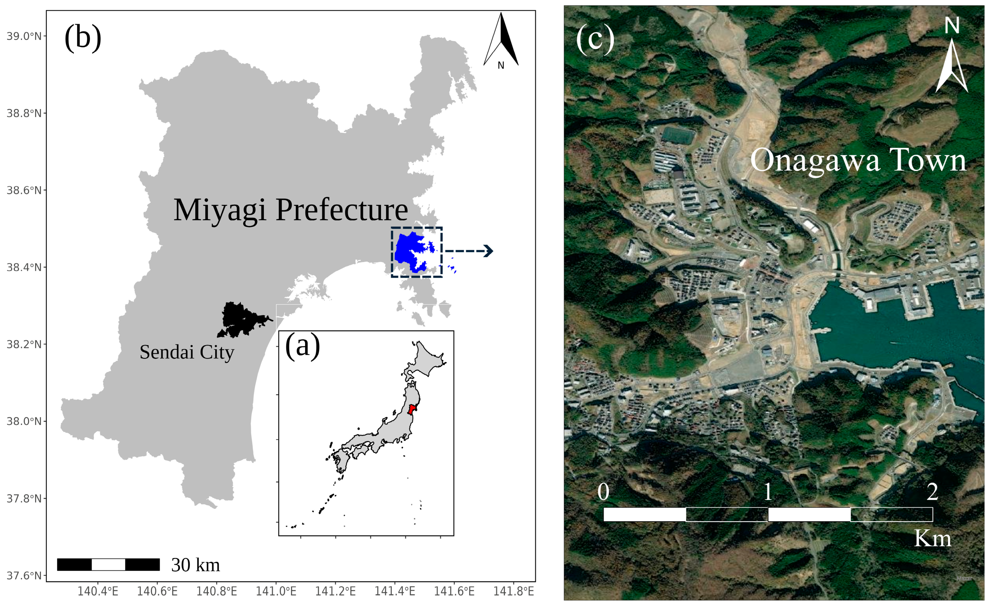
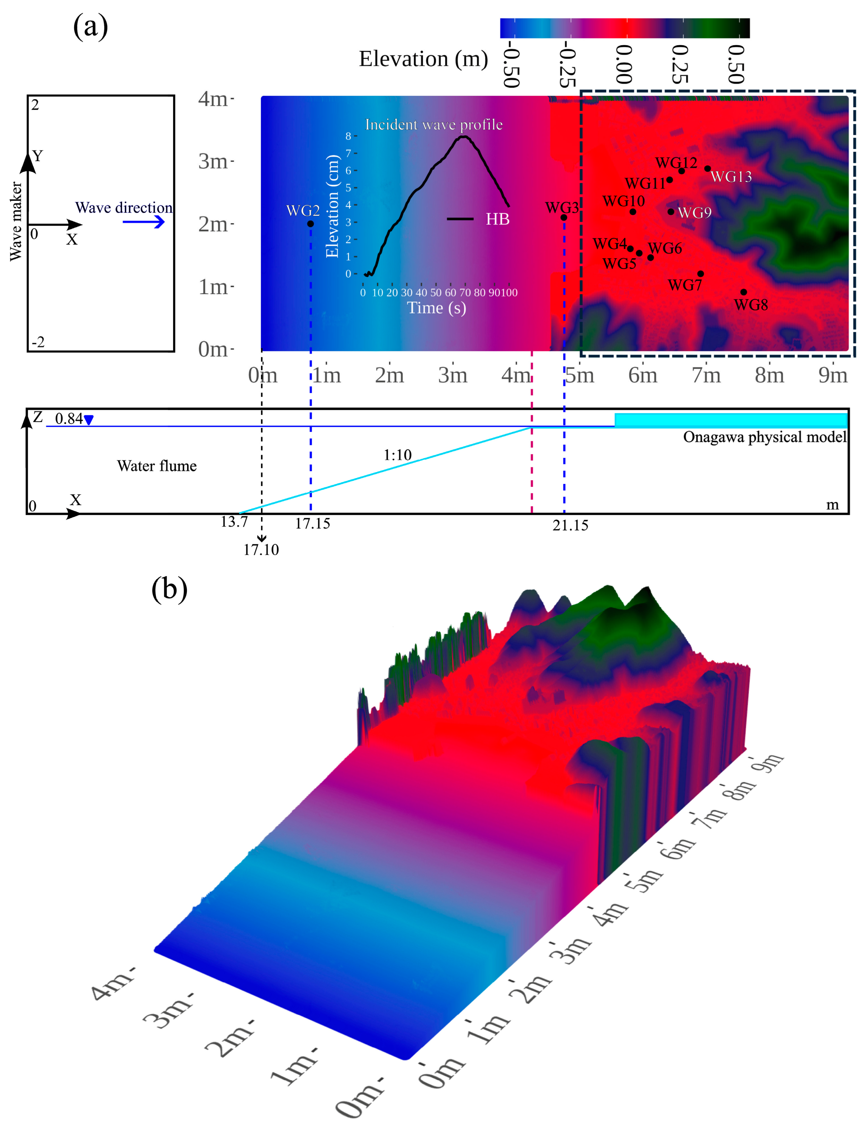
2.1. Onagawa Town Physical and Numerical Experiments

Figure 2 shows the layout of the physical wave flume of Onagawa town. The upper subpanel of Figure 2a depicts a bird’s eye view of the physical model with the wave gauge locations. The model was divided into two parts [27]. The southern part (WG4–WG8) has an elevation ranging between 0.009 and 0.024 m and features fewer structures. The northern part (WG10–WG13) ranges between 0.01 and 0.050 m and features dense structures. The lower subpanel in Figure 2a provides a cross-sectional view of the physical experimental flume. The experiments were conducted at the Ujigawa Open Laboratory of the Disaster Prevention Research Institute (DPRI), Kyoto University. The physical model was constructed based on the real bathymetric characteristics of Onagawa town before 2011, with a model scale of 1:250. Onagawa town was selected due to the size of the town and the experimental facility. The experimental flume is 45 m long, 4 m wide, and 2 m deep. Hence, the Onagawa model was constructed in the flume [27]. The shoreline of the model was placed 17.15 m from the wavemaker. The shoreline of the model is a planar slide with a 1:10 bottom slope. The water depth in the water flume was set to 0.84 m.

Two incident wave profiles were imposed at the left open boundary: the hydraulic bore (HB) and the solitary wave (SW) types. In Prasetyo et al.’s study [27], the 2D nonlinear shallow-water equation model and the quasi-3D (Q3D) model of the regional ocean model system (ROMS) were applied to test their efficiency in reproducing the inundation process by comparing their numerical results with those obtained from experimental flume results. In Q3D, the fully 3D governing equations deployed in the ROMS model were approximated by introducing a parameterised scheme of the vertical velocity in two dimensions. Hence, the flow was horizontally homogeneous within each vertical layer. In the 2D model, the grid size was 1 cm. In Q3D, the horizontal grid interval was 4 cm, and sigma coordinates with 10 layers were used in the vertical direction. The roughness coefficient (n) in their study was calculated based on the Manning model and was 0.025 for the seaward section and 0.013 for the landward section [27].

For the numerical experiment, the Onagawa terrain and an approximately 4 m long piece of the slope panel section were transformed into numerical data using a scanner with 1 mm resolution [27]. Therefore, the wave time series at WG2 (the boundary of the domain from the sea section side) was used as the input wave profile for the 2D and Q3D numerical models. Figure 2b depicts the 3D layout of the physical model that represents the slope in the sea section. According to Prasetyo et al. [27], in the HB case, the tsunami wave propagates following the slope and reaches the shoreline at WG4. A target maximum inundation depth of 7.62 cm at 69.6 s was successfully achieved in this experiment. In the SW case, the maximum inundation depth was approximately achieved at WG4, with 7.77 cm at 14.65 s. Then, propagation proceeded to inundate the entire town. The study concluded that the HB wave reasonably represented the 2011 Tohoku tsunami compared to the SW. Several studies have been conducted using the same wave flume at Kyoto University, and they have illustrated the efficiency of the experimental flume in producing robust results [5,6,33].

2.2. Open-Source Flow Solver

Basilisk, the next generation of Gerris, is an open-source flow solver designed for partial differential equations (PDEs) on adaptive cartesian meshes. This section describes the three approaches employed for the SV, SGN, and ML equations. For further information, refer to [13,28,30] and the Basilisk official website http://basilisk.fr/ (accessed on 31 October 2023).

2.2.1. Saint-Venant (SV) Solver

The SV equations are well known for their efficiency in determining fluid motion with a free surface elevation and vanishingly small water depth [28]. The equations are modelled and discretised on a hyperbolic system of conservation laws. Hence, fluid motion is simulated on a 2D quadtree mesh via the vertical integration of the horizontal components of water velocity [28,29]. Many studies have proven the efficacy of this approach when paired with the Gerris flow solver in determining tsunami propagation nearshore where long wave approximation with negligible water depth is valid [28,29,32,34,35].

The source term is presented as follows:

$$\partial t\underset{\partial \Omega }{\overset{}{\int }}qd\Omega =\underset{\partial \Omega }{\overset{}{\int }}f\left(q\right)·nd\partial \Omega -\underset{\Omega }{\overset{}{\int }}hg·\nabla z_b$$

(1)

where $\Omega$ is the subset of space, $d\Omega$ is its boundary, n is the normal unit vector on the boundary, g is gravitational acceleration, and $z_b$ is the bathymetry. For the conservation of mass and momentum in the shallow-water context, $\Omega$ is a subset of the 2D space, and q and f are defined as follows:

$$q=\left(\begin{array}{c}h\\ h{u}_x\\ h{u}_y\end{array}\right), f\left(q\right)=\left(\begin{array}{cc}h{u}_x& h{u}_y\\ h{u}_x^2+(1/2)g{h}^2& h{u}_x{u}_y\\ h{u}_x{u}_y& h{u}_y^2+(1/2)g{h}^2\end{array}\right)$$

(2)

where h is the water depth, $u_x$ and $u_y$ are the horizontal velocity components, and g is gravitational acceleration with a flat bottom (bathymetry) assumption. An additional forcing term should be provided if the bottom is not flat. Thus, Equation (1) becomes

$$\partial t\underset{\partial \Omega }{\overset{}{\int }}qd\Omega =\underset{\partial \Omega }{\overset{}{\int }}f\left(q\right)·nd\partial \Omega -\underset{\Omega }{\overset{}{\int }}hg·\nabla z$$

(3)

where $z$ is the depth of the topography. This system of equations is hyperbolic and secures an entropy inequality, meaning that the gross energy $h{u}_x^2+\left(1/2\right)g{h}^2$ behaves physically with ($u_x, u_y$).

Additionally, the steady state, a solution to this system, ensures that the lake-at-rest condition is preserved; this parameter is defined as follows:

$$u=0, h+z=constant$$

(4)

For further information on the discretization approach deployed within Basilisk’s notations, including the flux computation and the time integral, refer to the research conducted by Kurganov and Levy [36].

2.2.2. Serre–Green–Naghdi (SGN) Solver

The SGN equations are interpreted as the expansion of the SV equations to the following order $K=\left({\mu }^2\right)$ for the shallowness parameter:

$$\mu =h_0^2/L^2$$

(5)

where $h_0$ is bathymetric depth and $L$ is horizontal length.

The SGN equations were obtained by adding the source term to the momentum equation of the SV. Thus, the SGN equations have a dispersive wave solution, as presented below:

$$\partial t\underset{\partial \Omega }{\overset{}{\int }}qd\Omega =\underset{\partial \Omega }{\overset{}{\int }}f\left(q\right)·nd\partial \Omega +\underset{\Omega }{\overset{}{\int }}Sd\Omega$$

(6)

where $\Omega$ is a proportion of 2D space, $\partial \Omega$ is the boundary of the space, and $n$ is the normal unit vector on $\partial \Omega$. Concerning the last SV source term, the mass and momentum, $q$ and $f,$ were obtained from Equation (2). S is given as

$$S=\left(\begin{array}{c}0\\ -gh{\partial }_x{z}_b+h((g/\alpha ){\partial }_x\eta -D_x)\\ -gh{\partial }_y{z}_b+h((g/\alpha ){\partial }_y\eta -D_y)\end{array}\right)$$

(7)

where $z_b$ is the bathymetry, $\eta =z_b+h$ is the free surface elevation, and α is the dispersive parameter, equal to 1.153 in the original discretization of the SGN in Basilisk. The parameter α controls the optimisation of the dispersive relation [37]. In Equation (7), the first component $gh\nabla z_b$ represents the original bathymetry forcing term of the SV equations, while the second term represents the dispersive version of the SGN approximation. The vector field D is expressed as

$$h\left(I+\alpha T\right)\left(D\right)=g/\alpha \nabla \eta +Q_1\left(u\right)$$

(8)

where I is the identity matrix, and $T$ and $Q_1$ are the second-order linear differential operators. This equation is numerically beneficial given that $T$ and $Q_1$ rely on the second spatial derivative of $D$ and $u$, respectively, while other versions include a third derivative [37]. For the definitions of $T$ and $Q_1$, refer to the work by Popinet [13]. The code implementation of the SGN within the Basilisk framework deploys a dimensionless breaking parameter [13]. When the slope of the free wave surface exceeds a threshold value for the breaking parameter, the dispersive properties of the SGN will be inhibited, and the SV solver will assume control of the calculations. During the experiments, we found that the threshold of the breaking parameter should be 0.1 or less to preserve the computational stability of the SGN solver.

2.2.3. Multilayer (ML) Solver

The conventional multilayer-based SV system consisted of independent layers with no mass exchange between layers. Each layer is presented according to its height and velocity. In Popinet’s work [30], a multilayer model was developed by introducing the vertical hydrodynamics of fluid layers. Thus, the system was converted into the incompressible Euler formulation by integrating the layer flow bounded by a free surface and bathymetry. The model was proven to provide an efficient solution on a global scale, such as that of the 2011 Tohoku tsunami [30], or on a local scale [38,39].

The governing equations of the incompressible Euler system with a semi-discrete approximation for multilayer flow bounded by a free surface and bathymetry are as follows:

$${\partial }_t{h}_k+\nabla ·{\left(hu\right)}_k=0$$

(9)

$${\partial }_t{\left(hu\right)}_k+\nabla ·{\left(huu\right)}_k=-g{h}_k\nabla \eta -\nabla {{(h}_{\varphi })}_k+{[\varphi \nabla \widehat{z}]}_k$$

(10)

$${\partial }_t{\left(hw\right)}_k+\nabla ·{\left(hwu\right)}_k=-{\left[\varphi \right]}_k$$

(11)

$$\nabla ·{\left(hu\right)}_k+{\left[\omega -u·\nabla \hat{z}\right]}_k=0$$

(12)

where $k$ is the layer index; $h_k$ is layer thickness; $u_k$ and $w_k$ are the horizontal and vertical velocity components, respectively; and ${\varphi }_k$ is the nonhydrostatic pressure divided by the fluid density.

The source code of the ML solver is divided into two separate libraries (hydrostatic and nonhydrostatic) within the framework of Basilisk [30]. The two libraries work concurrently to produce a solution. Therefore, setting $\varphi =0$ will return this case to the hydrostatic multilayer SV system. Additionally, the turbulence model was also adjusted by discretizing the vertical diffusion implicitly within the source code of the nonhydrostatic library (Popinet [30] (p. 6)).

In the case of a multilayer, the free surface elevation η is given by

$$\eta =z_b+\sum _k{h}_k$$

(13)

where $z_b$ is bathymetry. The height of each layer interface $\widehat{z}$ is

$${\widehat{z}}_{k+1/2}=z_b+\sum _{l=0}^k{h}_l$$

(14)

Compared to that in the SGN solver, the breaking of waves in the ML solver is controlled by a different notation, which guarantees a reduction in the vertical velocity when wave breaking occurs [30]. The breaking parameter in the nonhydrostatic mode is described by the wave-free surface slope and the maximum vertical velocity profile as follows:

$$w_k^{n+1}\leftarrow \mathrm{sign}(w_k^{n+1})\min (\left|w_k^{n+1}\right|,b\sqrt{g{\left|H\right|}_{\infty }})$$

(15)

where b is the dimensionless breaking parameter, which must be smaller than one, and $\sqrt{g{\left|H\right|}_{\infty }}$ describes the horizontal velocity of the breaking waves. In complex flow conditions, when waves strongly break, the above reduction might be inadequate for preserving the model. For improvement, a wave-free surface slope limiter was added to the nonhydrostatic solver [30]. Therefore, the dispersive properties of waves will not deactivate in the built-in model. Instead, the vertical velocity will be reduced to provide a satisfactory solution for wave breaking.

2.3. Quadtree Adaptive Mesh Refinement (AMR)

The framework of AMR in Basilisk relies on a tree-adaptive mesh to initiate efficient refinement levels while maintaining a stable Cartesian grid [40]. The tree-adaptive algorithm depends on two methods for ensuring stability and efficiency: prolongation (the interpolation of values from coarser cells to finer cells) and restriction (the interpolation of values from finer to coarser cells) by implementing nested loops [13]. Thus, the calculated values are automatically inherited from the parents’ cells to the children’s cells and vice versa through the simulation. The spatial derivative of the domain is assessed on the Cartesian grid by implementing so-called ghost cells, represented by stencils within the boundaries. The ghost cell values are interpolated from the field values, ensuring that all the cells have neighbouring cells [40]. The refinement evolution develops by a factor of two for each level of refinement.

2.4. Dynamic Terrain Reconstruction

The AMR method ensures satisfactory performance, as mentioned above. However, the adequate processing of a model’s bathymetry is required. In the constant Cartesian grid, bathymetry is defined and accessed only once as a prerequisite. In the AMR, the bathymetry database must be accessed at every timestep where a new level of refinement is created. At each new refinement level, the bathymetry is accessed and defined using the current finest level. To satisfy this refinement requirement, the bathymetry data must have a small memory footprint and be accessible at each time step [29]. The bathymetry cell is evaluated by splitting it into finer cells consistent with the tree adaptive mesh evolution, following the refinement procedure [40]. In this approach, two conditions should, in practice, be preserved: volume conservation and lake at rest. For tsunami modelling, preserving the lake at rest ensures better performance [29]. Thus, the condition $z_c={(z}_1+z_2)/2$ should be maintained at every refinement step. As a result, to implement these conditions, bathymetry reconstruction should be implemented backwards, beginning at the finest level where the bathymetry has yet to be defined.

2.5. Model Set-Up

The SV, SGN, and ML solvers were applied to a quadtree adaptive mesh. The simulation was run in parallel computing using an open MPI with 14 CPUs (E5-2609 v4 with 1.70 GHz). The code implementation is as follows:

(1)

The mesh refinement was set between min = 2⁶ (approximately 14 cm) and max = 2⁹ (approximately 1.8 cm);

(2)

A maximum simulation time of 100 s and a dry parameter of 0.1 mm were also applied;

(3)

In the case of the nonhydrostatic models, the CFL condition and the breaking parameter were defined;

(4)

The time series at WG2 was considered an incident wave profile following the same input wave used in the 2D and Q3D experiments [27];

(5)

The value of n was set to 0.025 for sea and 0.013 for land in wet cells, following the methods of Prasetyo et al. [27] for accurate comparison with the 2D and Q3D experiments.

Once the numerical model has been executed, mesh adaptation is launched with respect to two criteria: the estimation of the free surface error to track wave propagation and the estimation of the maximum wave height error for resolving the final maximum wave. First, we identify the water level $(eta;\eta =h+z_b only if h>dry)$ for each stencil. In the computation, the wet/dry contact line is represented by nested loops within each solver. A dry parameter is defined with a small value (0.1 mm), and at each iteration, a conditional statement is applied to determine if the water height is greater than the dry parameter in the cell. Thus, the wet/dry contact line is resolved for each iteration of the solver during the inundation process.

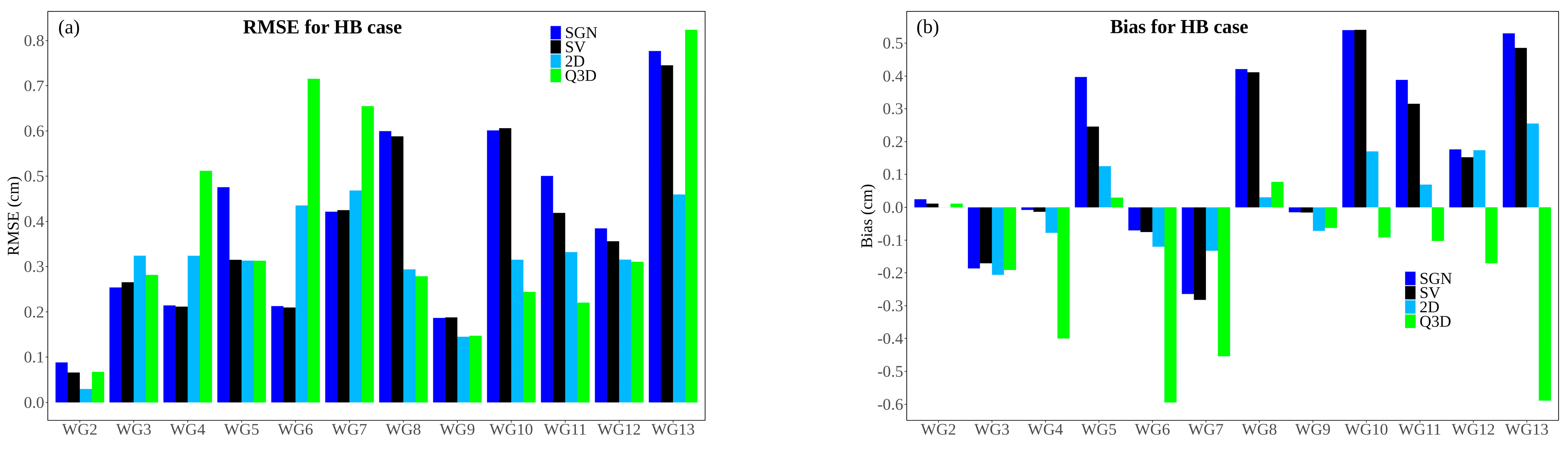
2.6. Statistical Metrics

To evaluate the performance of each solver, the following three statistical metrics were calculated to test the efficiency of reproducing the experimental tsunami-like waves when compared to that of the 2D and Q3D models from Prasetyo et al.’s work [27]. (i) the correlation coefficient (R); (ii) the root mean square error (RMSE) quantifies the typical deviation between the predicted values of the numerical models and the experimental flume values and can be expressed mathematically as the standard deviation of the model’s residuals; and (iii) bias (B) describes the degree to which the predicted values deviate from the actual values, either by consistently overestimating or underestimating the experimental values.

$$\mathrm{R}={\sum }_{i=1}^N({wo}_i-\overline{wo})({wm}_i-\overline{wm})/\sqrt{{\sum }_{i=1}^N{({wo}_i-\overline{wo})}^2{\sum }_{i=1}^N{({wm}_i-\overline{wm})}^2}$$

(16)

$$\mathrm{R}\mathrm{M}\mathrm{S}\mathrm{E}=\sqrt{\raisebox{1ex}{${\sum }_{i=1}^N{\left({wm}_i-{wo}_i\right)}^2$}\!\left/ \!\raisebox{-1ex}{$N$}\right.}$$

(17)

$$\mathrm{B}=\raisebox{1ex}{${\sum }_{i=1}^N{wm}_i-{wo}_i$}\!\left/ \!\raisebox{-1ex}{$N$}\right.$$

(18)

where ${wo}_i$ is the observed water elevation, $\overline{wo}$ is the mean observed value, ${wm}_i$ is the model value of the water elevation, $\overline{wm}$ is the mean model value, and $N$ is the sample size.

3. Results

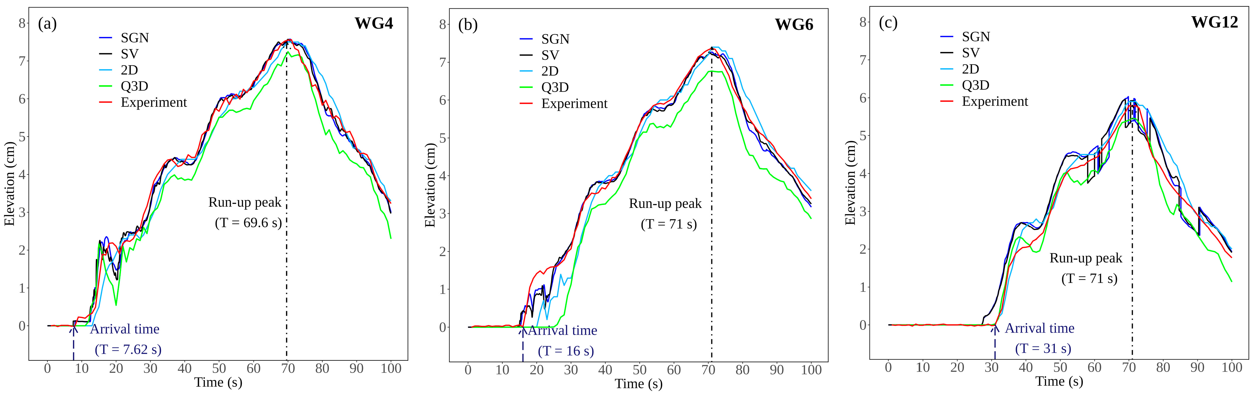
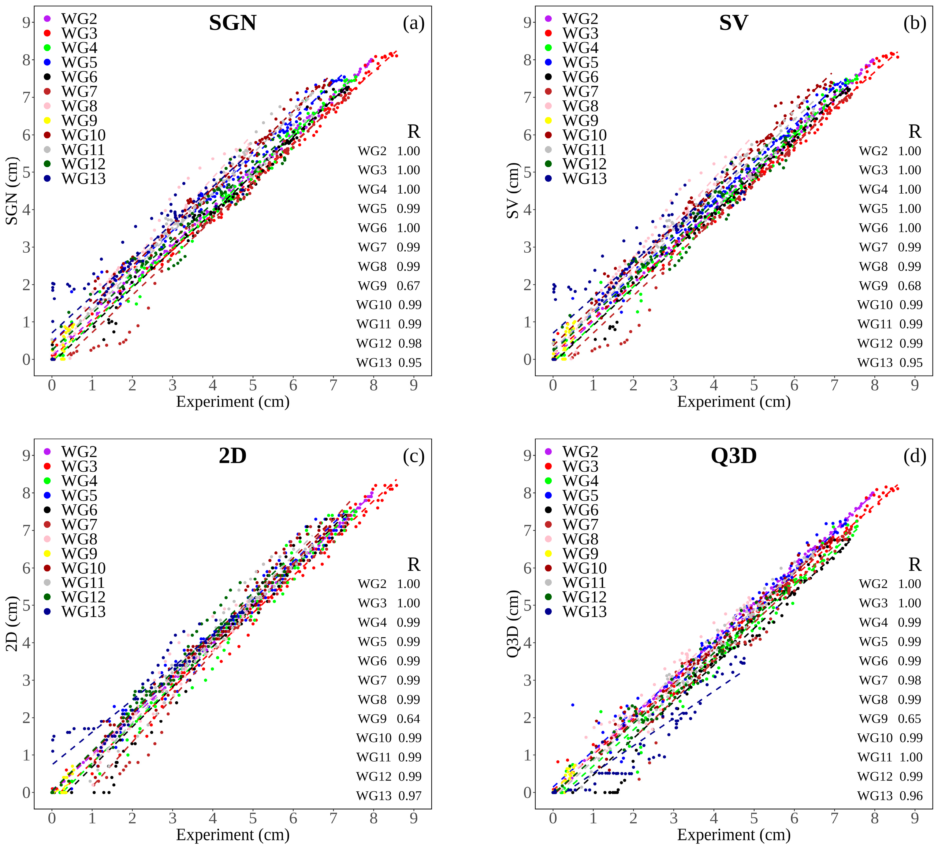
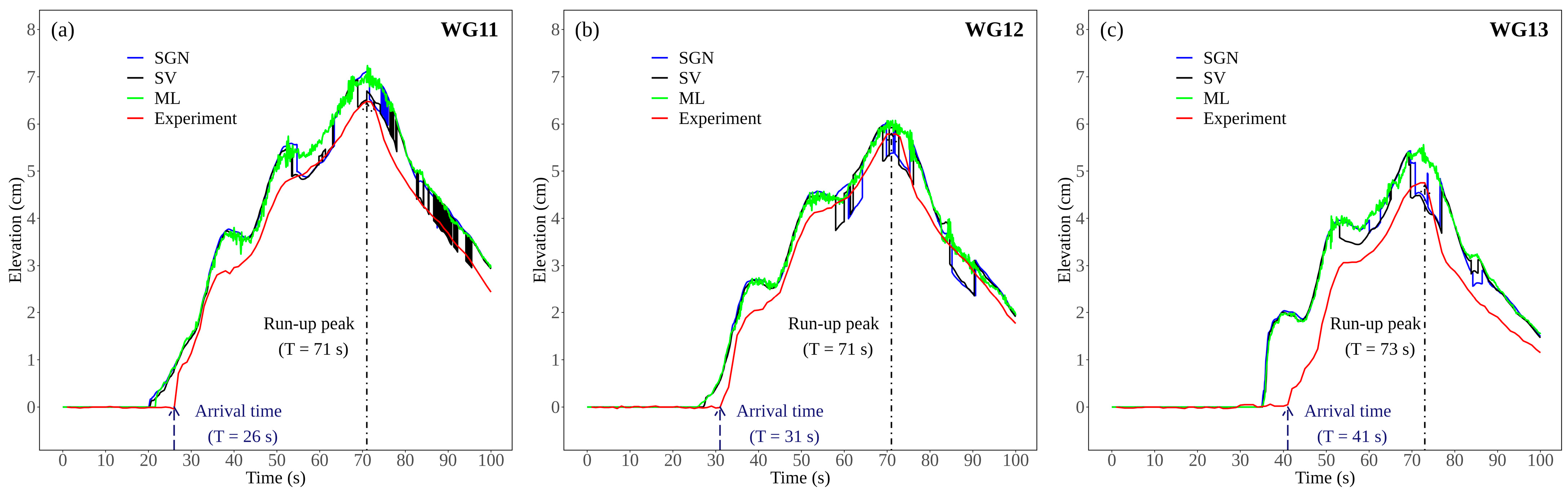
3.1. Validation Using Experimental Results

A tsunami-like hydraulic bore wave was generated in the experimental flume using a pump generator. The hydraulic bore wave was more realistic than the solitary wave in replicating the 2011 Tohoku tsunami event [27]. This simulation was conducted using SV and SGN solvers, and the results were validated against the experimental flume results (Figure 3).

As the wave propagated toward the shoreline, the adaptive mesh wavelet algorithm began refining the mesh to solve the inundation process. Figure 3a shows the time series at WG4, the first point onshore. The results from the SGN and SV models showed greater accuracy with respect to predicting the arrival time of the wave than those from the 2D and Q3D models. The tsunami’s arrival time was approximately 8 s, while in the 2D case, the wave arrived after approximately 13 s, and in the Q3D case, the wave arrived after approximately 11 s. In the Q3D case, the maximum wave height was approximately 3.1 mm lower than that in the experiment.

As the tsunami wave propagates further inside the built-in environment, the propagation cleaves into two parts, following the model terrain. The wave run-up in the southern part of the built-in model is depicted at WG6 in Figure 3b. The tsunami wave arrived at WG6 after approximately 16 s. The arrival time with respect to the SV model was approximately 15 s, and that for the SGN model was approximately 15.5 s. On the other hand, the arrival time in the case of the 2D model was over 20 s, and that in the Q3D model was over 25 s. The wave run-up height was not well captured in the case of Q3D, being approximately 6.25 mm less than that in the experiment. The performances of the SGN and SV models are almost identical because the dispersive properties of the SGN model are inhibited by the breaking parameter. This is also noticeable from the time series plots, where no oscillation was observed. The SGN solver provided a more accurate correlation with the experimental results due to the automatic intermittence of the breaking parameter [13]. Even though the AMR maximum resolution was less than that in 2D, the SGN and SV models exhibited improved performance in determining the arrival time and wave run-up heights.

The northern section of the Onagawa model has a higher altitude and denser structures than the southern part [27]; hence, the wave run-up height is lower in this section, and the arrival times were later for many structures. Figure 3c shows the tsunami time series comparison at WG12 in the northern section of the built-in environment. The arrival time in the SGN and SV models was approximately 27.5 s, while the actual arrival time was approximately 31 s. For almost all the wave gauges in the northern section, the arrival time was slightly earlier than that in the experiment due to interactions with complicated terrain and land structures. In the dense structure section, the waves broke continuously, and the narrow streets were more likely to form vortices. Additionally, the built-in section should be characterised by different types of bottom friction to include the effect of the structures on delaying the arrival time and reducing the run-up height. The SGN and SV models accurately ascertained the run-up height at WG12, while in the case of the Q3D, the maximum run-up height was 2.8 mm lower than that in the experiment. The results from the Q3D model illustrated inferior behaviour compared to the other models, particularly in simulating the run-up peak. The low performance of the Q3D model could be due to its rough spatial resolution, about 4 cm, compared to that of the 2D model, corresponding to 1 cm [27]. Watanabe et al. [8] also reported superior performance of the NSWE models over 3D models in terms of tsunami wave repeatability. However, the NSWE models also had finer resolution compared to the 3D models.

Figure 4a–d present scatter plots of the wave elevations at all wave gauges in the numerical models, SGN, SV, 2D, and Q3D, respectively, against the wave elevation in the physical experiment.

The mean R value for all the wave gauges in all the numerical models was approximately 0.96. The correlation was satisfactory for all the numerical models. WG9’s being situated on higher ground surrounded by hills places it in a complicated position for wave calculation (Figure 2). The wave arrived at WG9 after approximately 65 s, approximately 5 s before the maximum inundation. Thus, the maximum peak was simulated within 5 s of temporal resolution. As shown in Figure 4, the R value was lower at WG9 than at the other wave gauges. However, the SGN and SV models provided higher R values, namely, 0.67 and 0.68, than the 2D and Q3D models, which yielded values of 0.64 and 0.65, respectively. The RMSE of the SGN and SV data indicated good performance at WG3, WG4, WG6, and WG7 (Figure 5a). For WG8, the performance of the SGN and SV models decreased compared to that of the 2D and Q3D models. In the AMR method, the mesh adapts gradually (2⁶ → 2⁷ → 2⁸ → 2⁹) with propagation inland in wet cells. When the leading wave reaches the wave gauge location, the resolution is 2⁷. Hence, the rough resolution at the front line affects accurate detection. Furthermore, the n value in the built-in area is 0.013, which poorly reflects the potential situation. The wave gauges in the southern section (WG4–WG8) are on a road with fewer obstacles (see Figure 2a), and the wave gauges in the northern section (WG10–WG13) are surrounded by many obstacles. In Figure 5b, the bias ranged between −0.4 cm and 0.5 cm for the SGN and SV, with mostly underestimation of the experimental wave at WG3, WG4, WG6, WG7, and WG9 and overestimation at WG2, WG5, WG8, WG10, WG11, WG12, and WG13. On the other hand, the Q3D model mainly underestimated the experimental wave, producing overly low values, as shown in Figure 5b; the values were −0.6 cm at WG6 and WG13, as depicted in the time series comparison in Figure 3.

3.2. Nonhydrostatic Solutions

The simulation using the ML solver was conducted with two layers. The ML results coincided with the SGN and SV results in terms of detecting the arrival time in the southern section of the built-in model. Implementing the nonhydrostatic solver improved the overall wave run-up solution in the built-in model. Furthermore, the consistency of the solution was preserved, as illustrated by the presence of the run-up peak (Figure 6). In the northern section (corresponding to WG11, WG12, and WG13), the ML solver improved the results relatively. However, the arrival time and the run-up peak were not captured, especially at WG13. Despite the short longitudinal and latitudinal distances between the three wave gauges, wave propagation was significantly delayed, and the run-up height was also reduced due to the gradually increasing altitude and dense structures. The arrival times at WG11, WG12, and WG13 were 26 s, 31 s, and 41 s, respectively, and the run-up peaks were 6.45 cm, 5.8 cm, and 4.75 cm, respectively. Even by including the nonhydrostatic model, a maximum resolution of 2⁹ was used to resolve the propagation in the northern section. Applying a higher resolution on the order of 2¹¹ or more further improves the wave solution. However, the demanding computational capacity and the actual simulation time are drawbacks of this approach.

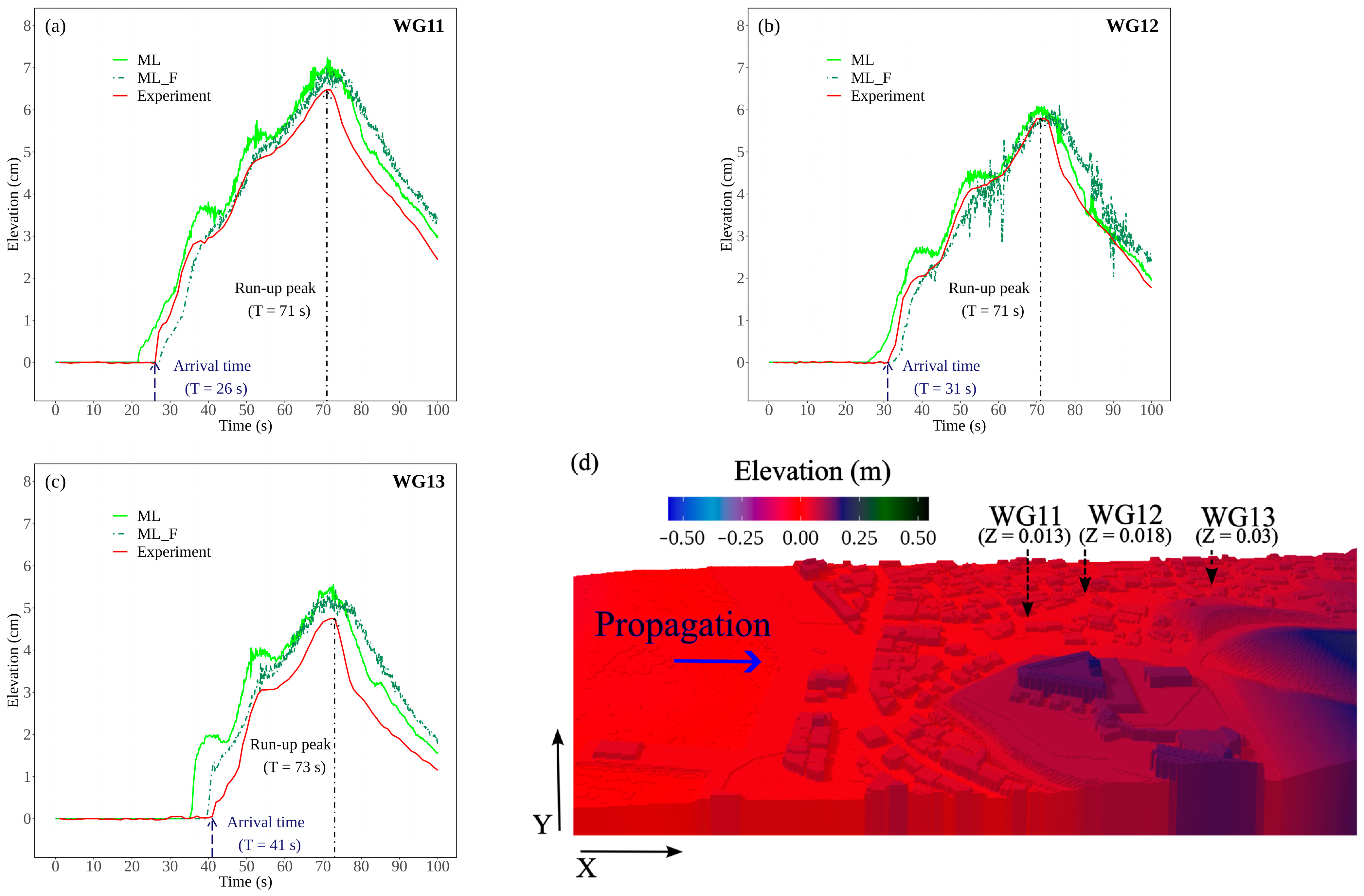
3.3. Improved n Using the ML Solver

The tsunami wave run-up is strongly affected by the density of the structures. Experimental studies have been carried out to examine the reduction in run-up height due to interactions with land structures [33,41]. According to Pracetyo et al. [27], the run-up height decreased by approximately 26% between WG11 and WG13. The increase in land obstacles resulted in the dissipation of wave energy, leading to a marked reduction in run-up height. The n values within urban environments and forested areas were observed to be inadequately low [33]. Many hydrologic models incorporate the surface roughness of land cover, accounting for various features like grass, small bushes, and pavement. These considerations lead to the assignment of smaller roughness coefficients, such as 0.013 for road and rail networks [42,43]. Using numerical models, Cardenas et al. [44] estimated the effect of increasing n values on the inundated area. These authors highlighted that a high n value leads to underestimation of the inundated area, and the arrival time is less affected by the change in n. However, the cited study considered a digital surface model for a city in Chile and did not focus on a microscale shoreland. A similar n approximation was obtained by Maruyama et al. [45] when studying the inundation process in Asahi city in Chiba Prefecture due to the 2011 Tohoku tsunami. Indeed, the inundation velocity and length will decrease significantly with an increasing n value, and such an effect should be considered. Therefore, the effect of macroroughness was considered separately for the northern section of the Onagawa model. The ML solver was used for the additional numerical experiment.

Figure 7 shows the time series comparison with the experimental flume measurements among the ML solvers before (ML) and after (ML_F) improvement. The n values for the landward of the Onagawa model were divided according to the section. For the southern section (WG4–W8), the value of 0.013 was preserved [46]. For the northern section, a linearly increasing n value with propagation was applied. For an elevation of 1–4 cm, the n value increased from 0.2 at the shoreline (X = 5 m) to approximately 0.58 at WG13. Large n values were proposed to accurately represent tsunami propagation in coastal cities with dense land structures [47]. Additionally, for the streets in the northern section, n was set to 0.05 [46]. The increasing n value in the northern section reflects a positive effect on wave propagation. The locations of WG11, 12, and 13 are shown in detail in Figure 7d. The dense structures acted as protection, causing a significant delay in the arrival time due to energy dissipation. An increased n value represents the macroroughness effect, resulting in an accurate wave solution, as depicted in the time series comparison in Figure 7a–c. Energy dissipation resulted in eddies in narrow streets, indicated by the dark red points on the left side in Figure 8. The ML successfully estimated the arrival time with a 1 s delay. However, the run-up peak was overestimated by 0.3 cm at WG11 and by 0.45 cm at WG13.

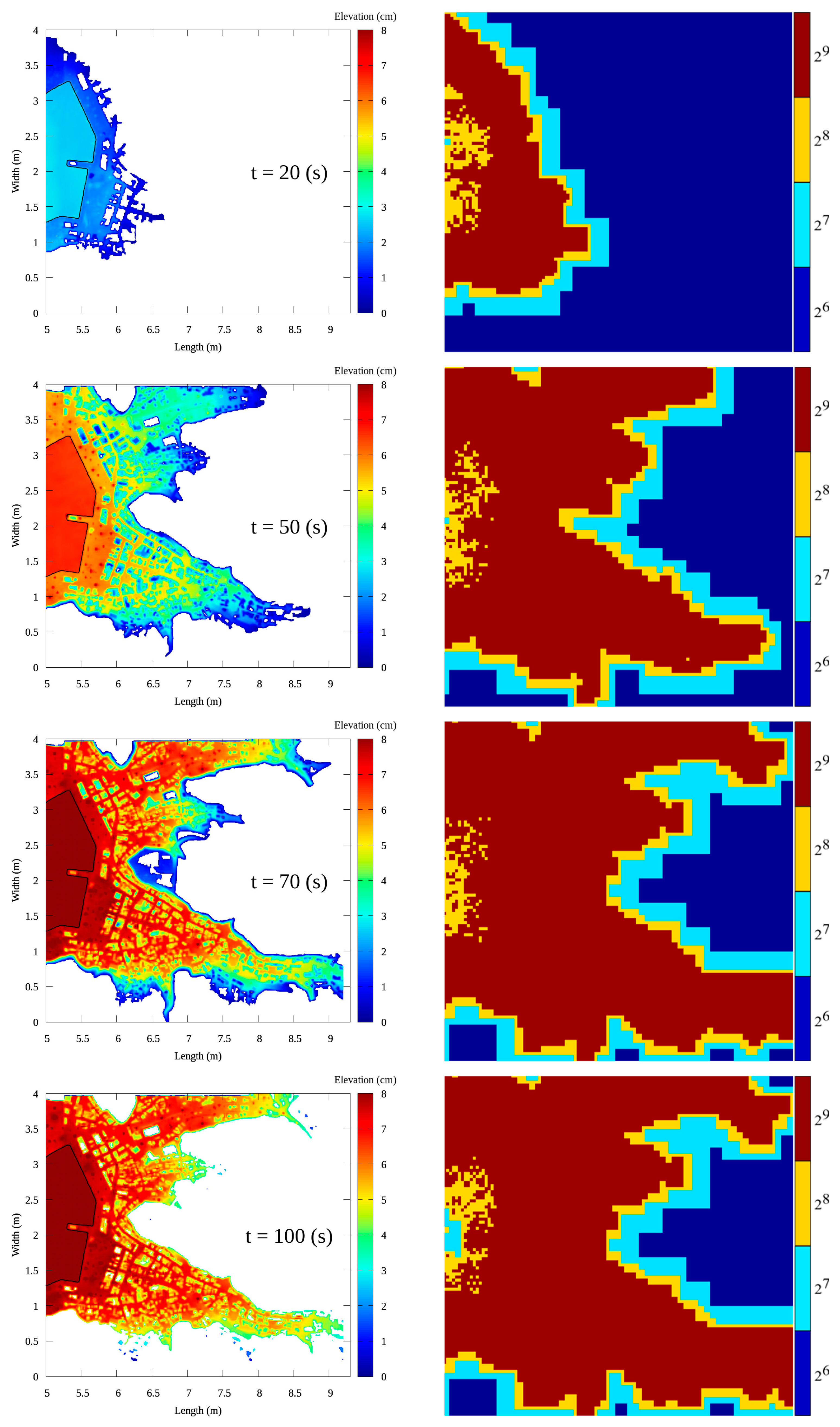
3.4. Spatial Inundation

Figure 8 shows the inundation process of the Onagawa physical model. Snapshots at 20 s (at which point the wave started to propagate in the built-in area), 50 s (at which point the wave arrived at all wave gauges except WG9), 70 s (the maximum wave run-up in the built-in area), and 100 s (the end of the simulation when water retreated to the sea section). Snapshots were taken from the ML_F solver after modifying the n values. The wave propagated directly in the southern section, where the built-in area is smoother than that in the northern section. After all the streets in the built-in area were gradually inundated, the maximum inundation progressed, as depicted in the second 50th row. The increasing wave run-up in complicated land structures formed eddies as the wave energy dissipated and the run-up height decreased.

The ML solver successfully captured the water surface oscillations and the whirlpools that formed during the process. The dark red points indicate the locations of the whirlpools. The right-hand column in Figure 8 shows the mesh refinement during the simulation. A Cartesian mesh of a level of 2⁶ was uniformly structured for the entire domain. As the wave propagated inland, the mesh was automatically refined, capturing the leading edge of the wave. Figure 8 shows that high resolution (2⁹) continued to be obtained in the built-in area even after the leading edge of the wave had further propagated. The hydrodynamic solution of the ML solver is the reason behind this behaviour. Water oscillation in wet cells demands high refinement. Thus, increasing the resolution will require greater computational capacity.

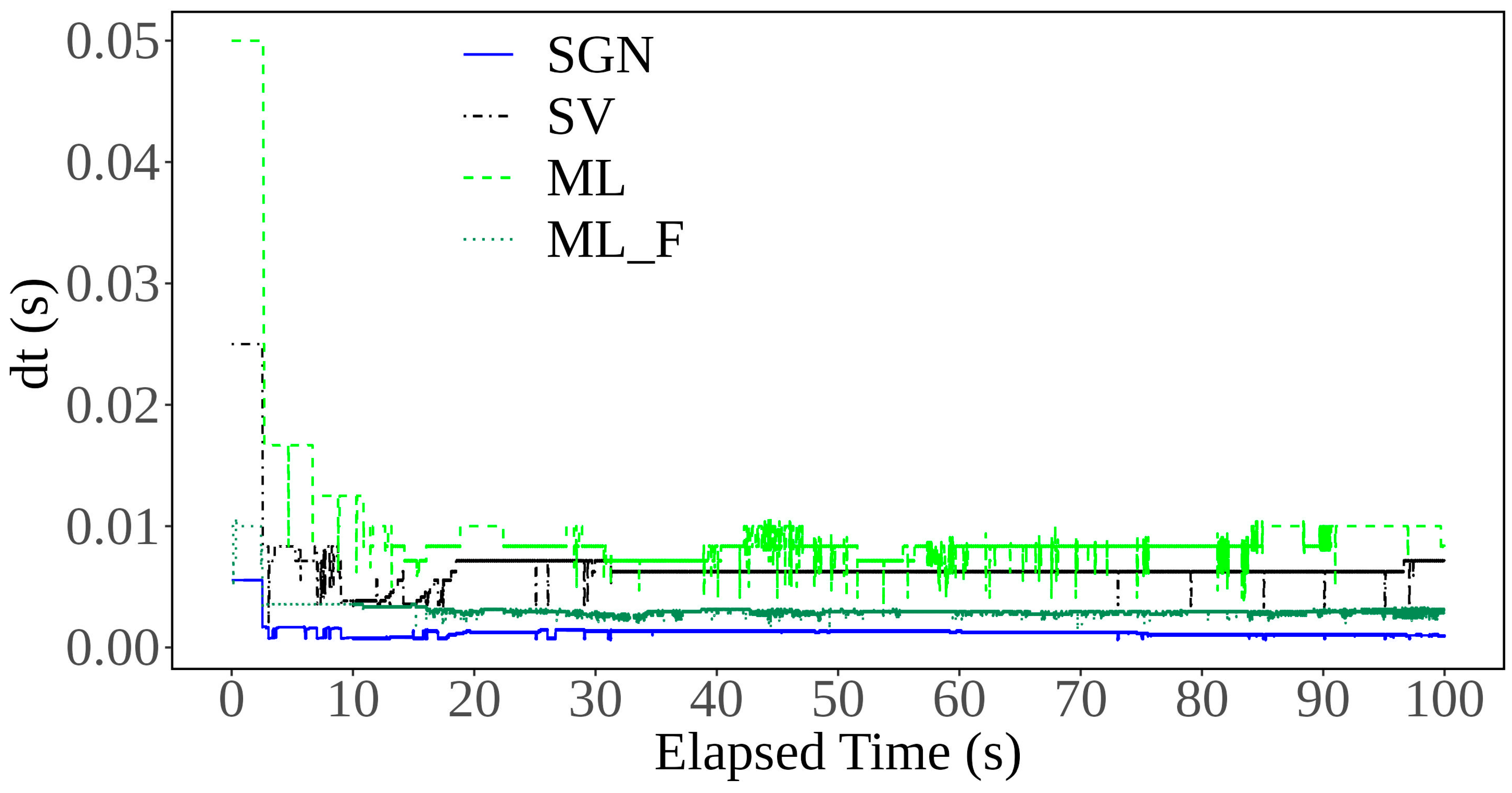
3.5. Computational Time Step

The computational time steps of all the models are depicted in Figure 9. dt shows the required time steps for each model to solve 100 s of tsunami propagation. As shown, the temporal resolution of the SGN solver was notably lower than that of the SV and ML models, amounting to approximately 0.0007. This is also illustrated in

Table 1. Comparison between the SGN, SV, ML, and ML_F models in terms of the time steps and the simulation time needed to solve 100 s of tsunami propagation.

Model	Time Steps	Simulation Time (h)
SGN	84,249	5.825
SV	16,060	0.93
ML	11,384	4.55
ML_F	33,522	12.94

, where the SGN model needed nearly 6 h to conduct the simulation. Due to the interaction with land structures in the built-in area, the waves break strongly and continuously. Since the SGN model is discretised to accommodate wave dispersiveness $K=\left({\mu }^2\right)$, the temporal resolution evolved into much smaller values. The SGN solver has been proven to accurately describe the perturbance of the water surface [13]. However, due to the corresponding large computational cost and difficulties in tuning dispersive parameters, the SGN solver is rarely used in tsunami propagation. The ML solver needed 11,384 time steps, the lowest value among all the models. As shown in Figure 9, the temporal resolution fluctuated around approximately 0.01 at the beginning of the simulation. After 20 s, the time steps fluctuated around 0.008. Due to the nonhydrostatic solution in the ML solver, the mesh refinement encompassed all wet cells, not solely the wave’s leading edge (see Figure 8). This ensured consistent wave propagation without sudden drops, better preserving wave continuity compared to the SV solver (see Figure 6). The temporal resolution of the SV solver was almost constant at approximately 0.0013 after 20 s. On the other hand, increasing the n value in the ML_F significantly affected temporal resolution and running time. A linearly increased n value requires finer time steps to preserve the CFL condition due to the velocity reduction. Thus, the needed computational capacity increased significantly after more than 12 h of simulation time, as shown in Table 1.

4. Discussion

The advantage of the AMR method lies in reducing the calculation time. In contrast to the constant grid, the refinement level evolves automatically between 2⁶ and 2⁹ refinement levels. Hence, the computational capacity will be concentrated at a specific location where the mesh is refined during the simulation to solve the wave propagation problem instead of consuming computational time and effort in the entire domain. Blaise et al. [48] developed an SV model with adaptive unstructured mesh on a spherical coordinate system. The developed model was validated with real tsunami events and emphasised the efficiency of the adaptive mesh in reducing the simulation time compared to a uniform grid. Another AMR adaptation was presented by Pons et al. [49,50]. Indeed, the AMR method enhanced the simulation efficiency with a reduction in computational time. However, the implementation of the AMR method with nonhydrostatic models to study tsunami inundation in complex coastal areas remains a thriving topic.

To investigate the abovementioned advantages of the AMR method alone, two independent numerical experiments were conducted using the SV solver. The SGN and the ML solver consumed a remarkable amount of time on AMR. Hence, running on a constant grid is not recommended. The first numerical experiment was conducted on a multigrid (constant grid) with a resolution of 2⁹, and the second was conducted on a quadtree adaptive mesh with a resolution varying from 2⁶ to 2⁹.

Table 2. Comparison of the computation times of the SV solver with a constant grid and an AMR in the case of the hydraulic bore.

Type of the Grid	Refinement Level	Time Steps	Simulation Time (h)
Constant grid	29	28,024	6.8
AMR	26 ≤ AMR ≤ 29	16,060	0.93

presents a comparison between the two experiments. The simulation with a constant grid consumed 28,024 time steps and lasted 6.8 h, while the simulation with AMR consumed 16,060 time steps and lasted 0.93 hr. The AMR method reduced the simulation time by approximately 86.3% compared to that of the constant grid. This efficiency makes the AMR method more dependable in real-time forecasting and early-warning systems. However, further comparisons with other numerical tsunami models regarding computational efficiency are recommended.

5. Conclusions

A numerical experiment on tsunami inundation in a complex coastal zone conducted by Prasetyo et al. [27] was reproduced to assess the efficiency of AMR with nonhydrostatic models using the Basilisk open-source flow solver and to emphasise the importance of n in simulating tsunami inundation in a complex coastal environment. Three numerical models were run over a quadtree adaptive mesh, namely, models based on the Saint-Venant (SV) equation, the Serre–Green–Naghdi (SGN) equation, and a multilayer (ML) extension of the SGN equation.

The numerical experiments were conducted using a tsunami-like hydraulic bore wave in the original bathymetry model of Onagawa town since it reasonably represents the 2011 Tohoku tsunami that impacted the town. The results yielded by the SGN and SV models agreed well with the experimental results and were superior to the results yielded by the 2D and Q3D models. Furthermore, the Basilisk models were more efficient at predicting the arrival time in the built-in area of the Onagawa model. The dispersive version of the SGN model exhibited relatively good performance on the complex terrain of the built-in area. However, this approach is computationally more expensive.

Compared with the SGN and SV solvers, the ML solver provided a consistent solution for wave propagation. However, the arrival time and run-up peak in the northern section were not determined due to the rough resolution. An additional experiment was conducted with the ML solver after improving the n. A varying n was applied in the built-in area to reproduce the inundation more accurately. The n value in the southern section was 0.013. The n for the land structures in the northern section (for elevations between 1 and 4 cm) was set to increase linearly from 0.2 at X = 5 m, reaching approximately 0.58 at WG13. Additionally, a uniform n value of 0.05 was applied in the streets of the northern section. The results were enhanced by capturing the arrival time at the wave gauges in the northern section with an approximately 1 s delay.

The efficiency of the AMR method was scrutinised by running separate simulations on a constant grid using the SV solver. Compared with the constant grid, the simulation with AMR shortened the computational time by 86.3%.

Regarding tsunami uncertainty, understanding wave behaviour in urban areas is crucial in order to reduce mortality rates. Implementing the AMR method with nonhydrostatic solutions improves disaster prevention by allowing tsunami arrival times and run-up heights to be predicted more accurately in vulnerable coastal zones. However, the nonhydrostatic solution consumed a considerable amount of computational time compared to the hydrostatic models. The scope of this study could be extended further by evaluating the performance of the numerical models with real-scale tsunami inundation studies.

References

1. Goto, K.; Chagué-Goff, C.; Fujino, S.; Goff, J.; Jaffe, B.; Nishimura, Y.; Richmond, B.; Sugawara, D.; Szczuciński, W.; Tappin, D.R.; et al. New insights of tsunami hazard from the 2011 Tohoku-oki event. Mar. Geol. 2011, 290, 46–50. [Google Scholar] [CrossRef]
2. Mori, N.; Takahashi, T.; Yasuda, T.; Yanagisawa, H. Survey of 2011 Tohoku earthquake tsunami inundation and run-up. Geophys. Res. Lett. 2011, 38, L00G14. [Google Scholar] [CrossRef]
3. Kron, W. Coasts: The high-risk areas of the world. Nat. Hazards 2013, 66, 1363–1382. [Google Scholar] [CrossRef]
4. Mukherjee, A.; Cajas, J.C.; Houzeaux, G.; Lehmkuhl, O.; Suckale, J.; Marras, S. Forest density is more effective than tree rigidity at reducing the onshore energy flux of tsunamis. Coast. Eng. 2023, 182, 104286. [Google Scholar] [CrossRef]
5. Chida, Y.; Mori, N. Numerical modeling of debris transport due to tsunami flow in a coastal urban area. Coast. Eng. 2023, 179, 104243. [Google Scholar] [CrossRef]
6. Fukui, N.; Prasetyo, A.; Mori, N. Numerical modeling of tsunami inundation using upscaled urban roughness parameterization. Coast. Eng. 2019, 152, 103534. [Google Scholar] [CrossRef]
7. Sugawara, D. Numerical modeling of tsunami: Advances and future challenges after the 2011 Tohoku earthquake and tsunami. Earth-Sci. Rev. 2021, 214, 103498. [Google Scholar] [CrossRef]
8. Watanabe, M.; Arikawa, T.; Kihara, N.; Tsurudome, C.; Hosaka, K.; Kimura, T.; Hashimoto, T.; Ishihara, F.; Shikata, T.; Morikawa, D.S.; et al. Validation of tsunami numerical simulation models for an idealized coastal industrial site. Coast. Eng. J. 2022, 64, 302–343. [Google Scholar] [CrossRef]
9. Khakimzyanov, G.; Dutykh, D.; Fedotova, Z. Dispersive shallow water wave modelling. Part III: Model derivation on a globally spherical geometry. Commun. Comput. Phys. 2018, 23, 315–360. [Google Scholar] [CrossRef]
10. Khakimzyanov, G.; Dutykh, D.; Gusev, O.; Shokina, N. Dispersive shallow water wave modelling. Part II: Numerical simulation on a globally flat space. Commun. Comput. Phys. 2018, 23, 30–92. [Google Scholar] [CrossRef]
11. Khakimzyanov, G.; Dutykh, D.; Gusev, O. Dispersive shallow water wave modelling. Part IV: Numerical simulation on a globally spherical geometry. Commun. Comput. Phys. 2018, 23, 361–407. [Google Scholar] [CrossRef]
12. Khakimzyanov, G.; Dutykh, D.; Fedotova, Z.; Mitsotakis, D. Dispersive shallow water wave modelling. Part I: Model derivation on a globally flat space. Commun. Comput. Phys. 2018, 23, 1–29. [Google Scholar] [CrossRef]
13. Popinet, S. A quadtree-adaptive multigrid solver for the Serre-Green-Naghdi equations. J. Comput. Phys. 2015, 302, 336–358. [Google Scholar] [CrossRef]
14. Glimsdal, S.; Pedersen, G.K.; Harbitz, C.B.; Løvholt, F. Dispersion of tsunamis: Does it really matter? Nat. Hazards Earth Syst. Sci. 2013, 13, 1507–1526. [Google Scholar] [CrossRef]
15. Dias, F.; Milewski, P. On the fully-nonlinear shallow-water generalized Serre equations. Phys. Lett. Sect. A Gen. At. Solid State Phys. 2010, 374, 1049–1053. [Google Scholar] [CrossRef]
16. Shi, F.; Kirby, J.T.; Harris, J.C.; Geiman, J.D.; Grilli, S.T. A high-order adaptive time-stepping TVD solver for Boussinesq modeling of breaking waves and coastal inundation. Ocean Model. 2012, 43–44, 36–51. [Google Scholar] [CrossRef]
17. Lynett, P.J.; Wu, T.-R.; Liu, P.L.-F. Modeling wave runup with depth-integrated equations. Coast. Eng. 2002, 46, 89–107. [Google Scholar] [CrossRef]
18. Xu, W.J.; Dong, X.Y. Simulation and verification of landslide tsunamis using a 3D SPH-DEM coupling method. Comput. Geotech. 2021, 129, 103803. [Google Scholar] [CrossRef]
19. Sarfaraz, M.; Pak, A. SPH numerical simulation of tsunami wave forces impinged on bridge superstructures. Coast. Eng. 2017, 121, 145–157. [Google Scholar] [CrossRef]
20. Aslami, M.H.; Rogers, B.D.; Stansby, P.K.; Bottacin-Busolin, A. Simulation of floating debris in SPH shallow water flow model with tsunami application. Adv. Water Resour. 2023, 171, 104363. [Google Scholar] [CrossRef]
21. Reis, C.; Barbosa, A.R.; Figueiredo, J.; Clain, S.; Lopes, M.; Baptista, M.A. Smoothed particle hydrodynamics modeling of elevated structures impacted by tsunami-like waves. Eng. Struct. 2022, 270, 114851. [Google Scholar] [CrossRef]
22. Dai, Z.; Li, X.; Lan, B. Three-Dimensional Modeling of Tsunami Waves Triggered by Submarine Landslides Based on the Smoothed Particle Hydrodynamics Method. J. Mar. Sci. Eng. 2023, 11, 2015. [Google Scholar] [CrossRef]
23. Liang, Q.; Borthwick, A.G.L.; Stelling, G. Simulation of dam- and dyke-break hydrodynamics on dynamically adaptive quadtree grids. Int. J. Numer. Methods Fluids 2004, 46, 127–162. [Google Scholar] [CrossRef]
24. Gisler, G.R.; Weaver, R.P.; Mader, C.L.; Gittings, M.L. Two- and three-dimensional asteroid impact simulations. Comput. Sci. Eng. 2004, 6, 46–55. [Google Scholar] [CrossRef]
25. Behrens, J.; Bader, M. Efficiency considerations in triangular adaptive mesh refinement. Philos. Trans. R. Soc. A Math. Phys. Eng. Sci. 2009, 367, 4577–4589. [Google Scholar] [CrossRef] [PubMed]
26. Leveque, R.J.; George, D.L.; Berger, M.J. Tsunami modelling with adaptively refined finite volume methods. Acta Numer. 2011, 20, 211–289. [Google Scholar] [CrossRef]
27. Prasetyo, A.; Yasuda, T.; Miyashita, T.; Mori, N. Physical modeling and numerical analysis of tsunami inundation in a coastal city. Front. Built Environ. 2019, 5, 46. [Google Scholar] [CrossRef]
28. Popinet, S. Adaptive modelling of long-distance wave propagation and fine-scale flooding during the Tohoku tsunami. Nat. Hazards Earth Syst. Sci. 2012, 12, 1213–1227. [Google Scholar] [CrossRef]
29. Popinet, S. Quadtree-adaptive tsunami modelling. Ocean Dyn. 2011, 61, 1261–1285. [Google Scholar] [CrossRef]
30. Popinet, S. A vertically-Lagrangian, non-hydrostatic, multilayer model for multiscale free-surface flows. J. Comput. Phys. 2020, 418, 109609. [Google Scholar] [CrossRef]
31. Audusse, E.; Bristeau, M.O.; Perthame, B.; Sainte-Marie, J. A multilayer Saint-Venant system with mass exchanges for shallow water flows. Derivation and numerical validation. ESAIM Math. Model. Numer. Anal. 2011, 45, 169–200. [Google Scholar] [CrossRef]
32. Lee, H.S.; Shimoyama, T.; Popinet, S. Impacts of tides on tsunami propagation due to potential Nankai Trough earthquakes in the Seto Inland Sea, Japan. J. Geophys. Res. Oceans 2015, 120, 6865–6883. [Google Scholar] [CrossRef]
33. Tomiczek, T.; Prasetyo, A.; Mori, N.; Yasuda, T.; Kennedy, A. Physical modelling of tsunami onshore propagation, peak pressures, and shielding effects in an urban building array. Coast. Eng. 2016, 117, 97–112. [Google Scholar] [CrossRef]
34. Shimoyama, T.; Lee, H.S. Tsunami-Tide Interaction in the Seto Inland Sea, Japan. Coast. Eng. Proc. 2014, 1, 2. [Google Scholar] [CrossRef]
35. Lee, H.S.; Komaguchi, T.; Yamamoto, A.; Hara, M. Wintertime Extreme Storm Waves in the East Sea: Estimation of Extreme Storm Waves and Wave-Structure Interaction Study in the Fushiki Port, Toyama Bay. J. Korean Soc. Coast. Ocean. Eng. 2013, 25, 335–347. [Google Scholar] [CrossRef]
36. Kurganov, A.; Levy, D. Central-upwind schemes for the Saint-Venant system. Math. Model. Numer. Anal. 2002, 36, 397–425. [Google Scholar] [CrossRef]
37. Bonneton, P.; Chazel, F.; Lannes, D.; Marche, F.; Tissier, M. A splitting approach for the fully nonlinear and weakly dispersive Green-Naghdi model. J. Comput. Phys. 2011, 230, 1479–1498. [Google Scholar] [CrossRef]
38. Battershill, L.; Whittaker, C.N.; Lane, E.M.; Popinet, S.; White, J.D.L.; Power, W.L.; Nomikou, P. Numerical simulations of a fluidized granular flow entry into water: Insights into modeling tsunami generation by pyroclastic density currents. J. Geophys. Res. Solid Earth 2021, 126, e2021JB022855. [Google Scholar] [CrossRef]
39. Hayward, M.W.; Whittaker, C.N.; Lane, E.M.; Power, W.L.; Popinet, S.; White, J.D.L. Multilayer modelling of waves generated by explosive subaqueous volcanism. Nat. Hazards Earth Syst. Sci. 2022, 22, 617–637. [Google Scholar] [CrossRef]
40. van Hooft, J.A.; Popinet, S.; van Heerwaarden, C.C.; van der Linden, S.J.A.; de Roode, S.R.; van de Wiel, B.J.H. Towards Adaptive Grids for Atmospheric Boundary-Layer Simulations. Bound. Layer Meteorol. 2018, 167, 421–443. [Google Scholar] [CrossRef]
41. Goseberg, N. Reduction of maximum tsunami run-up due to the interaction with beachfront development-Application of single sinusoidal waves. Nat. Hazards Earth Syst. Sci. 2013, 13, 2991–3010. [Google Scholar] [CrossRef]
42. Papaioannou, G.; Efstratiadis, A.; Vasiliades, L.; Loukas, A.; Papalexiou, S.M.; Koukouvinos, A.; Tsoukalas, I.; Kossieris, P. An operational method for Flood Directive implementation in ungauged urban areas. Hydrology 2018, 5, 24. [Google Scholar] [CrossRef]
43. Kalyanapu, A.J.; Burian, S.J.; Mcpherson, T.N. Effect of land use-based surface roughness on hydrologic model output. J. Spat. Hydrol. 2009, 9, 51. [Google Scholar]
44. Cárdenas, G.; Catalán, P.A. Accelerating Tsunami Modeling for Evacuation Studies through Modification of the Manning Roughness Values. GeoHazards 2022, 3, 492–508. [Google Scholar] [CrossRef]
45. Maruyama, Y.; Kitamura, K.; Yamazaki, F. Estimation of tsunami-inundated areas in Asahi City, Chiba Prefecture, after the 2011 Tohoku-oki earthquake. Earthq. Spectra 2013, 29, 201–217. [Google Scholar] [CrossRef]
46. De Jong, H. River Flood Damage Assessment Using Ikonos Imagery; JRC: Ispra, Italy, 2001; Available online: https://www.researchgate.net/publication/40218937 (accessed on 4 January 2024).
47. Gayer, G.; Leschka, S.; Nöhren, I.; Larsen, O.; Gänther, H. Tsunami inundation modelling based on detailed roughness maps of densely populated areas. Nat. Hazards Earth Syst. Sci. 2010, 10, 1679–1687. [Google Scholar] [CrossRef]
48. Blaise, S.; St-Cyr, A. A dynamic hp-Adaptive discontinuous Galerkin method for shallow-water flows on the sphere with application to a global tsunami simulation. Mon. Weather Rev. 2012, 140, 978–996. [Google Scholar] [CrossRef]
49. Pons, K.; Ersoy, M. Adaptive Mesh Refinement Method. Part 1: Automatic Thresholding Based on a Distribution Function. 2019. Available online: https://hal.science/hal-01330679v2 (accessed on 4 January 2024).
50. Pons, K.; Ersoy, M.; Golay, F.; Marcer, R. Adaptive Mesh Refinement Method. Part 2: Application to Tsunamis Propagation. 2019. Available online: https://hal.science/hal-01330680v3 (accessed on 4 January 2024).
Figure 1. (a) Map of Japan with the location of Miyagi Prefecture; (b) Miyagi Prefecture, with Onagawa town in the northeast of the prefecture facing the Pacific Ocean; and (c) an aerial image of Onagawa town, which was built between the mountains with a valley connecting to the Pacific Ocean, taken after the 2011 Tohoku Tsunami event.
Jmse 12 00177 g001
Figure 2. (a) The layout of the Onagawa physical model in the experimental wave flume along with the locations of the wave gauges, WG1–WG13, in the model. The incident wave profile for the hydraulic bore (HB) is imposed at the left boundary. The dashed box is the focused built-in area for the inundation study. (b) A 3D layout of the Onagawa model used for numerical experiments (9.2 × 4 m), depicting the terrain surrounding the town and the slope toward the wavemaker.
Jmse 12 00177 g002
Figure 3. Time series comparison between SGN, SV, 2D, and Q3D and the physical experiment at (a) WG4, (b) WG6, and (c) WG12.
Jmse 12 00177 g003
Figure 4. Scatter plots with correlation coefficient (R) values of all waves with respect to the experimental results: (a) SGN, (b) SV, (c) 2D, and (d) Q3D.
Jmse 12 00177 g004
Figure 5. Comparisons of the (a) RMSE and (b) bias results among the SGN, SV, 2D, and Q3D methods at all the wave gauges.
Jmse 12 00177 g005
Figure 6. Comparison of water level time series among the SGN, SV, ML, and experimental flume results at the locations of (a) WG11, (b) WG12, and (c) WG13.
Jmse 12 00177 g006
Figure 7. Comparison of water level time series among ML (before improving n), ML_F (after improving n), and the experiment at the locations of (a) WG11, (b) WG12, and (c) WG13. (d) The location of the three wave gauges in the northern section.
Jmse 12 00177 g007
Figure 8. Snapshots of the wave propagation and the mesh refinement level with regard to the ML_F solver in the focused built-in area for the inundation study. The left column shows the tsunami wave propagation throughout the built-in area of the Onagawa model at 20, 50, 70, and 100 s. The right column illustrates the mesh refinement levels used to detect the change in the water surface precisely in the entire domain.
Jmse 12 00177 g008
Figure 9. Comparison of the computational time steps of the SGN, SV, ML, and ML_F models.
Jmse 12 00177 g009