Development of a Mobile Buoy with Controllable Wings: Design, Dynamics Analysis and Experiments

Abstract

Marine monitoring equipment such as Argo profiling buoys and underwater gliders are important devices for oceanographic research and marine resource exploration. In this study, a novel mobile buoy capable of vertical profiling motion like Argo profiling buoys and sawtooth gliding motion like underwater gliders is proposed. The proposed mobile buoy can switch between the two motion modes with controllable wings. To verify the feasibility of the proposed mobile buoy, a fluid–multibody coupling model considering multibody dynamics and hydrodynamics was developed to investigate the dynamic response. A scaled-down buoy prototype was fabricated and the feasibility of the two motion modes was experimentally investigated in a laboratory tank. The experimental results agree well with the results of numerical simulation. This work can be helpful for the design and analysis of this kind of mobile buoy.

1. Introduction

Oceanographic observation is the foundation of marine science research. The vastness and complexity of the ocean make oceanographic observation extremely challenging. Autonomous surface/underwater vehicles provide an efficient way to monitor the marine environment with lower consumption, higher spatial–temporal resolution and longer-range transport, showing significant advantages over the previous oceanographic observation technology and contributing to the development of ocean observations [1]. According to the observation requirements in different sea areas and depths, a variety of autonomous vehicles, such as profiling buoys, underwater gliders, remotely operated vehicles and autonomous underwater vehicles, have been developed and are gradually forming a global ocean observation network [2].

In recent years, Argo profiling buoys and underwater gliders, with the outstanding advantages of superior autonomy, long endurance and low consumption, have attracted the attention of marine research scholars. Argo profiling buoys can accurately measure ocean profile data, such as temperature and salinity, through periodical profiling motion in the vertical direction [3]. Thanks to its simple structure and long working time, Argo profiling buoys can acquire and send data regularly and frequently throughout the year, independent of weather conditions, and the temporal coverage of the Argo data is much better than that of ship monitoring [4,5]. However, traditional Argo profiling buoys are poorly maneuverable and can only drift with the ocean currents rather than moving autonomously along the desired trajectory, making it difficult to cross ocean eddies, ocean fronts or some other stirring dynamic regions [6]. To improve the maneuverability of the buoys, researchers have considered equipping buoys with a propulsion apparatus [7]. Zoss et al. [8] proposed a self-propelled buoy with propellers that is highly maneuverable and excellently seaworthy, but it has to be acknowledged that it is not suitable for long-distance travel. The SOTAB-I proposed by Senga et al. [9] allows vertical and horizontal motions through buoyancy control device and thrusters. However, the SOTAB-I is still not suitable for long-distance travel due to the use of propellers. To improve long-distance travel, the SOTAB-II [10] uses a sail and oscillating fins to control the buoy motion. Due to the use of sails and oscillating fins, the mechanics of SOTAB-II is more complex than other traditional buoys. Furthermore, the sail is highly affected by the wind, resulting in a less controllable buoy. Yu et al. [11] proposed a low-cost mobile buoy that utilizes wind sails and water sails to propel the buoy movement, which has a relatively simple mechanical structure and is suitable for long-distance sailing, and it is not easy to achieve vertical uplift and dive.

Compared to traditional buoys, underwater gliders can overcome relatively small ocean currents and actively travel hundreds of kilometers, allowing them to acquire oceanographic data from the desired sea area [12,13]. The underwater glider can perform sawtooth gliding motion and reliable trajectory tracking by adjusting the buoyancy and the position of the center of gravity. The forward motion is driven by the horizontal component of the lift force generated by the glider wing [14]. Although underwater gliders with good maneuverability have shown excellent performance in monitoring the ocean environment, their endurance is often limited to a few months, far less than the long term of the Argo profiling buoys [15,16].

Generally, Argo profiling buoys, such as APEX buoys [17], Deep-Argo buoys [5] and Arvor buoys [18], are typically deployed by a mother ship into the target sea area for oceanic observations within a confined region. The traditional profiling buoys are capable of conducting vertical profiling observations by sinking and floating, but lack the ability to move horizontally, and can only drift with the waves. The underwater glider, such as Spray [19], Slocum [20] and Seaglider [21], is an automatic underwater vehicle that moves vertically by changing buoyancy and horizontally using wings. It can conduct observations in a long range, but it lacks the ability to perform vertical profiling observations. If the positive attributes of multiple autonomous surface/underwater vehicles can be combined, then the multifarious and continuous observation of ocean can be achieved. Recently, the field of cooperation observation by multitype vehicles has emerged, changing the status of vehicles with a single mode and satisfying the needs of comprehensive observation [22,23]. Given that the motion of Argo profiling buoys is uncontrollable, while the underwater glider observations can be planned, a combination of Argo profiling buoys and underwater gliders is proposed to perform network sampling of the ocean [24]. However, the implementation of multiple types of vehicles working together in one system poses a significant challenge to the control capabilities of the system. In addition to the above approaches, researchers have tried to explore underwater vehicles with multiple motion capabilities. For example, a multimodal underwater vehicle with a specially designed attitude control system and ingenious general arrangement that allows switching between buoying and gliding modes [25]. Zhou et al. [26] presented a conceptual design of a multimodal underwater vehicle carrying a propeller/rudder to correct the heading deviation caused by the mode transition. Then, a mathematical model that can fully describe the two operation modes is established based on the quaternion method, revealing the deviation of the heading angle in the switching between Argo mode and zigzag gliding mode. Liu et al. [27] proposed a dual-modal vehicle named Petrel-Dual, which can navigate in different modes on the surface and underwater. This vehicle has the ability to convert the harvested wind energy into a propulsion force for surface navigation, and can be pushed by diving or climbing in underwater navigation by its own net buoyancy and hydrodynamic lift. Multimodal underwater vehicles certainly contribute to ocean monitoring by providing a large amount of data collected from different locations.

The harmonious integration of different underwater vehicles into a single well-functioning system poses a great challenge for the associated theoretical analysis and control. A dynamic model is essential to analyze the dynamic characteristics of underwater vehicles. With the advent of high-computational computers, dynamic models of gliders have been rapidly developed. Yang et al. [28] established a six-dof (six degrees of freedom) parameterized dynamic model of the Petrel-L glider and explored the effects of wing location and net buoyancy on turning maneuverability and gliding stability. Wang et al. [29] developed the dynamics model of gliders using dual quaternions to solve the “gimbal lock” problem caused by the increased pitch angle range, which furtherly enriched the motion modes of the glider. The effective dynamic model is crucial for evaluating the motion response and stability of marine buoys. Yang et al. [30] considered the influence of sea water density variations and developed a nonlinear dynamic model for deep-sea profiling buoys, which provides a theoretical foundation for effectively controlling the vehicle. Zhu and Yoo [31] considered the dynamics of the cables and buoy in the numerical model and established the model of the buoy by numerical integration algorithms, aiming to illustrate the relationships between these motions and the propagating waves. In the research process of underwater vehicles, accurate hydrodynamic analysis is essential for dynamic modeling and motion performance analysis. Based on large eddy simulation and the Ffowcs–Williams and Hawkings equations, Qin et al. [32] performed hydrodynamic analysis for a Slocum glider and a blended-wing-body glider, and concluded that blended-wing-body gliders have lower energy cost and low noise performance. Le and Hong [33] used computational fluid dynamics (CFD) methods to acquire the hydrodynamic characteristics of a torpedo-shaped underwater glider, demonstrating the practicality of CFD methods in glider design. To reflect the underwater glider motion more realistically, Wang et al. [34] proposed a fluid–multibody coupled analysis method considering the interactions between multibody dynamics and fluid dynamics, enabling a complex dynamic analysis of the underwater glider.

Inspired by the characteristics of Argo profiling buoys and underwater gliders, a novel mobile buoy is proposed in this study. Figure 1 shows the working scheme of the proposed mobile buoy, which can navigate with Argo or glider operating modes by rotating the wings at a certain angle. In Argo mode, long-term observations can be carried out in a low-power way by drifting with the ocean currents, and oceanographic data such as temperature and salinity can be obtained. Considering the influence of ocean eddies and ocean fronts on the observation, the wing can be controlled to rotate at a certain angle to switch to Glider mode, which could correct the drift introduced by environmental disturbance through horizontal displacement.

The features and contributions of the proposed mobile buoy can be summarized as follows: (1) A novel mobile buoy design that breaks the limitation of using propellers to improve buoy maneuverability, making low-energy operation possible. Moreover, it can realize the mode switch through controlling wing rotation instead of the attitude control system, simplifying the internal structure and facilitating control and operation. (2) A fluid–multibody coupling model considering the interplay of the mobile buoy and the fluid, which analyzes the dynamics characteristics of the mobile buoy in two motion modes.

This paper is organized as follows. Section 2 introduces the working principle and the design of the mobile buoy. Section 3 develops a fluid–multibody coupling method considering the multibody dynamics and hydrodynamics to investigate the dynamic response of the mobile buoy. In Section 4, the dynamic characteristics of the proposed mobile buoy in Argo mode and Glider mode are discussed, mainly concerning the vertical profile movements and sawtooth gliding motions. Section 5 describes the tank experiment results for verifying the feasibility of the proposed mobile buoy concept and fluid–multibody coupled analysis method. Finally, some conclusions and future work are summarized in Section 6.

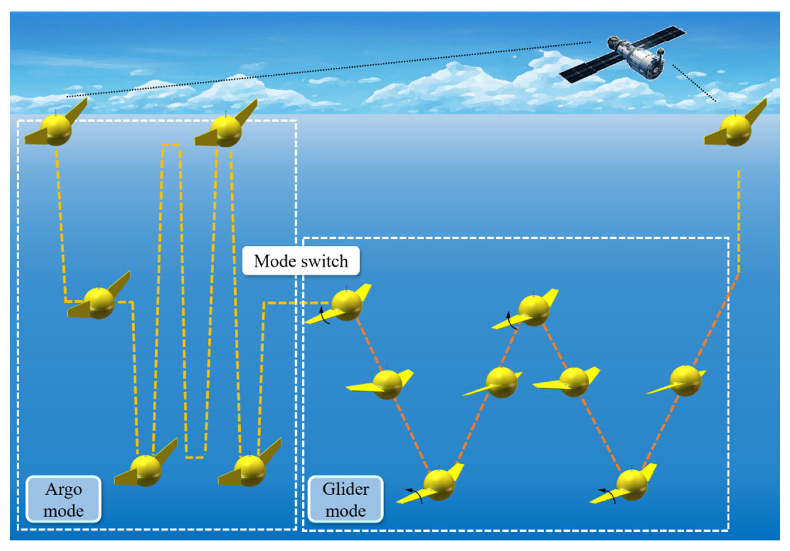
2. Mobile Buoy with Controllable Wings

The proposed mobile buoy aims to obtain a higher level of integration between a buoyancy-driven underwater glider and a conventional Argo profiling buoy, making it more compact and easier to perform continuous observations at a multiscale range. Figure 2a shows the shape and internal structural design of the mobile buoy. The internal structure of the buoy is identical to that of a conventional underwater glider, primarily comprising a buoyancy regulating system, control system and battery components. Unlike conventional underwater gliders, the attitude of the proposed mobile buoy can be controlled by adjusting the rotation angle of the wings, thus switching between Argo mode and Glider mode. To describe the rotational state of the wing clearly, the definition of wing rotation angle α_w is introduced in Figure 2b. The longitudinal axis of the fuselage (L-axis) coincides with the direction of antenna installation, and the horizontal axis of the fuselage (H-axis) that along the central axis of the spherical pressure shell is perpendicular to the L-axis. α_w is the wing rotation angle (the angle where the wing axis intersects with the H-axis). During underwater navigation, the mobile buoy achieves up and down motion driven by the net buoyancy and is propelled forward by the horizontal lift component acting on wings. In this paper, two operation modes are divided by the range of wing rotation angles: Argo mode (−80° ≤ α_w ≤ −90° or 80° ≤ α_w ≤ 90°) and Glider mode (0° < α_w ≤ −80° in climbing, 0° < α_w ≤ 80° in diving) by regulating α_w to control the ratio of horizontal displacement to diving depth to change the glide angle, as shown in Figure 2b. To ensure that the hydrodynamic forces acting on the fuselage are consistent in all directions, the shape of the mobile buoy is designed as a circular sphere consisting of two hemispherical pressure shells, thus contributing to the stability of the mobile buoy in both two motion modes. Stability is a critical aspect in the design process, which needs a reasonable arrangement of the internal configuration. For the proposed mobile buoy, the center of gravity is under the center of buoyancy and both are located on the same vertical line. In addition, the batteries and associated hardware of the buoyancy regulating system can be arranged at the bottom of the mobile buoy, which can provide the restoring moment to improve stability.

In the previous studies of buoys and underwater vehicles, most of them improved the maneuverability of the buoys by equipping mobility apparatuses and propellers, or enabled multi-mode integration for the vehicles through complex control systems, without considering the use of controllable wings to achieve simpler integration with profiling buoys and underwater gliders. In this study, a novel mobile buoy with controllable wings was developed to combine the positive attributes of Argo profiling buoy and underwater glider. The novel mobile buoy can achieve forward motion by utilizing the horizontal component of wing lift, which is different from prior research focused on enhancing buoy maneuverability through the addition of propellers. Meanwhile, it also overcomes the limitation of high energy consumption associated with traditional mobile buoys during propeller propulsion. Moreover, it simplify the internal structure by controlling wing rotation for operating modes switching, which is different from previous designs of multimode underwater vehicles.

3. Fluid–Multibody Coupling Dynamics Model

3.1. Fluid–Multibody Coupling Analysis Method

For the mobile buoy, hydrodynamics and multibody dynamics are two aspects that must be considered in their dynamics analysis. In this research, a fluid–multibody coupling method that incorporates both multibody dynamics and hydrodynamics model is developed to analyze the dynamic responses of the designed mobile buoy. The detailed procedure of the fluid–multibody coupling analysis is illustrated in Figure 3. Firstly, based on the initial motion condition (the dynamics equations of the mobile buoy at the initial moment) and the boundary condition (the boundary condition of the hydrodynamics model), the original mobile buoy is set within a presumed boundary region and meshed. Subsequently, hydrodynamic analysis is conducted within the CFD software. During this process, the macro commands DEFINE_CG_MOTION and Compute_Force_And_Moment function are applied via the UDF (user-defined function) of ANSYS-Fluent (15.0 version, ANSYS Corporation, Canonsburg, PA, USA) to compute the continuity equations and Navier–Stokes continuity equations, allowing for the determination of the hydrodynamic forces and moments exerted upon the mobile buoy. Then, the hydrodynamic force and moment are incorporated into its dynamics equation via the UDF codes to derive the accelerations and angular accelerations. By incorporating positions, attitudes, and accelerations of the mobile buoy can be obtained, enabling the extraction of the motion information for the next time step. This information is then used to update the mesh and motion through dynamic mesh technology. Subsequently, the mobile buoy is reintroduced into the hydrodynamics section and iterative calculations are performed. Through continuous motion state updates, fluid–multibody coupling analysis is conducted in the flow field. After all the time steps are calculated, the dynamic responses of the mobile buoy can be acquired. Compared to other methods that directly incorporate hydrodynamics into the multibody dynamic equations using empirical formula, the fluid–multibody coupling method takes time-varying hydrodynamics into account, enabling to reflect the motion state more objectively and realistically.

The continuity equation and Navier–Stokes equation for calculating hydrodynamic forces and moments exerted upon the mobile buoy can be expressed as

$${\displaystyle \underset{CS}{\iint }\rho \mu \cdot dS+\frac{\partial }{\partial t}}{\displaystyle \underset{CV}{\iiint }\rho dV=0}$$

(1)

$$\rho {\overline{u}}_j\frac{\partial {\overline{u}}_i}{\partial x_j}=\rho {\overline{f}}_i+\frac{\partial }{\partial x_i}\left[-\overline{p}{\delta }_{ij}+\mu (\frac{\partial {\overline{u}}_i}{\partial x_j}+\frac{\partial {\overline{u}}_j}{\partial x_i})\right]-\rho \overline{u_i{}^{\prime }{u}_j{}^{\prime }}$$

(2)

where ρ is the fluid density, μ is the velocity vector and S represents the characteristic area of the buoy. V is the volume, t is the time. u_i is the velocity component of the fluid, u_i′ is the pulsation velocity, f_i is the external force component acting on the fluid, μ is the dynamic viscosity and p is the pressure.

3.2. Multibody Dynamics Model of the Mobile Buoy

To describe the motion of the proposed mobile buoy, three coordinate frames are defined according to the standard method [35], as shown in Figure 4, including the inertial frame E-XYZ, the body frame e-xyz and the velocity frame e’-x’y’z’. The inertial frame is anchored to a reference point on the water surface, which be used to describe the position and attitude of the buoy. The initial heading of the mobile buoy on the water surface is the X-axis of the inertial frame, the Z-axis is vertically downward along the direction of the gravity and the Y-axis can be defined by the right-hand rule. The body frame is fixed to the wing, and its origin e is fixed to the center of buoyancy of the mobile buoy. The x-axis of the body frame points to the bow of the buoy along the axis of the wing, the z-axis is perpendicular to the x-axis and the y-axis can be acquired by the right-hand rule. As for the velocity frame, the origin coincides with the body frame, and the x’ axis points to the velocity direction. The z’ axis is vertically downward to the x’ axis in the plane e-xz. The direction of the y’ axis is obtained by the right-hand rule. With reference to the inertial frame, the position and the attitude of the mobile buoy are described by position vector b = [x, y, z] and angle vector η = [ϕ, θ, ψ], respectively. In the body frame, the velocity and the angular velocity of mobile buoy can be defined as V = [u, v, w] and Ω = [p, q, r], respectively. Moreover, the assumptions about the motion of the mobile buoy are given as follows: (1) The mobile buoy has six degrees of freedom, including surge, sway, heave, roll, pitch and yaw, where the dynamic response of the surge, heave and pitch degrees of freedom are focused on to assess the performance of the vehicle in profiling motion and the other degrees of freedom are ignored. (2) In this study, external disturbances such as wind, waves and currents, which are influenced by non-ideal environmental conditions, are not taken into consideration.

The angle which the body frame rotates around the Y-axis of the inertial frame can be expressed by φ.

$$\phi ={\alpha }_w+\theta$$

(3)

where α_w is the wing rotation angle and θ represents the pitch angle. In the diving phase of the mobile buoy, both α_w and θ are positive, and in the climbing phase of the mobile buoy, both α_w and θ are negative.

There is a specific mapping relationship between the variables in the inertial frame and the variables in the body frame, and the velocity vector of the mobile buoy in the inertial frame can be expressed as:

$$\dot{\mathit{b}}=\left(\begin{array}{l}\dot{X}\\ \dot{Y}\\ \dot{Z}\end{array}\right)=\left(\begin{array}{l}{V}_x\\ V_y\\ V_z\end{array}\right){=\mathit{R}}_E^B\left(\begin{array}{l}u\\ v\\ w\end{array}\right)$$

(4)

where V_x, V_y and V_z represent the velocities of the mobile buoy along the X-axis, Y-axis and Z-axis, respectively, all within the inertial frame. ${\mathit{R}}_E^B$ is the rotation matrix that maps the variables in the body frame to the inertial frame, which can be expressed as:

$${\mathit{R}}_E^B=\left(\begin{array}{ccc}\cos \psi \cos \phi & \cos \psi \sin \phi \sin \varphi -\sin \psi \cos \varphi & \cos \psi \sin \phi \cos \varphi +\sin \psi \sin \varphi \\ \sin \psi \cos \phi & \sin \psi \sin \phi \sin \varphi +\cos \psi \cos \varphi & \sin \psi \sin \phi \cos \varphi -\cos \psi \sin \varphi \\ -\sin \phi & \cos \phi \sin \varphi & \cos \phi \cos \varphi \end{array}\right)$$

(5)

The velocity of the mobile buoy in the inertial frame can be expressed as:

$$V=\sqrt{V_{\mathrm{x}}^2+V_{\mathrm{y}}^2+V_z^2}$$

(6)

The geometric structure of the mobile buoy can be regarded as a multibody system, as shown in Figure 5, which can be divided into three parts: the hull mass m_h (assuming a uniform distribution), the nonuniformly distributed mass m_w and the variable ballast mass m_b. The body frame, designated e-xyz, originates e at the geometric center (GC), which is the application point for the buoyancy and moments. The point mass m_h is simplified and positioned at GC, which are regarded as rigid mass points during the modeling. m_w is located at r_w with respect to the GC, providing a restoring moment that allows the proposed mobile buoy to return to the original equilibrium position after an external interference. The variable mass m_b (water in the tank) is the adjustable mass, considered as a mass point with constant position (located in GC) and variable mass, which can control the diving and climbing of the proposed mobile buoy by adjusting the buoyancy. Thus, the total mass m_t can be expressed as:

$$m_t=m_h+m_w+m_b$$

(7)

Normally, the effect of seawater density variation on buoyancy control is negligible. In this case, the mobile buoy substitutes a fixed water volume, and its mass can be represented as m. Thus, the net buoyancy mass m₀ in the water can be represented as follows:

$$m_0=m_{\mathrm{t}}-m$$

(8)

The motion of the mobile buoy in the vertical plane is an important way to obtain the oceanographic information. Figure 6 shows the forces acting on the mobile buoy as it moves in the vertical plane. F_d and F_l are the drag force and the lift force exerted on the mobile buoy in the flow field, respectively, which can be expressed as:

$$F_l=F_{l-fin}+F_{l-fuselage}$$

(9)

$$F_d=F_{d-fin}+F_{d-fuselage}$$

(10)

where F_l-fin is the lift force acting on the wings, F_l-fuselage is the lift force acting on the fuselage. F_d-fin is the drag force of the wings. F_d-fuselage is the drag force of the fuselage. The horizontal hydrodynamic forces acting on the proposed mobile buoy can be obtained by projecting F_d and F_l, which can be calculated as:

$$F_{x-fluid}=F_l\sin \gamma +F_d\cos \gamma$$

(11)

$$F_{z-fluid}=F_l\cos \gamma +F_d\sin \gamma$$

(12)

where γ represents the glide angle. F_x-fluid represents the hydrodynamic force in the X-axis direction and F_z-fluid is the hydrodynamic force in the Z-axis direction.

The forward motion is generated by the combined effect of lift and drag, and the propulsive force in X-axis direction is mainly provided by the horizontal component of the wing lift. During the Argo mode, when the wings of the mobile buoy are erected, the angle of attack is approximately 90°, causing the lift generated by the wing to be small or even negligible according to Rayleigh’s lift formula [36]. Therefore, the mobile buoy lacks horizontal displacement capability due to the horizontal component of lift being ignored, and can only perform vertical diving and climbing in an attitude of near vertical motion. During the Glider mode, the wing rotation angle α_w can be controlled to ensure the horizontal component of the lift is sufficient to generate the forward propulsive force, thus driving the mobile buoy forward. The equations of motion in both horizontal and vertical directions can be formulated as:

$$m_t\frac{d^{2}x}{d{t}^2}=F_{x-total}=F_{x-fluid}=F_l\sin \gamma +F_d\cos \gamma$$

(13)

$$m_t\frac{d^{2}z}{d{t}^2}=F_{z-total}=F_{z-fluid}+m_{0}g=F_l\cos \gamma +F_d\sin \gamma +m_{0}g$$

(14)

where F_x-total represents the resultant force in the direction of the X-axis, F_z-total represents the resultant force in the direction of the Z-axis. The horizontal displacement of the mobile buoy is represented by x, while its vertical displacement is represented by z.

The pitch motion equation of the mobile buoy can be expressed as:

$$I\frac{d\theta {(t)}^2}{d{t}^2}=M_{total}=M_{fluid}-m_{w}g{\mathit{r}}_w\sin \theta$$

(15)

where M_total is the resultant moment. M_fluid is the hydrodynamic moment. I represents the inertia of the mobile buoy concerning the y-axis, affecting the pitching motion of the buoy.

3.3. Hydrodynamics Model of the Mobile Buoy

The computational domain and boundary conditions of the hydrodynamics model is shown in Figure 7a. The entire computational domain is a cube with 10W × 10W × H. The inlet surface is 3W away from the model and is set as the velocity inlet, which was controlled by the UDFs based on Equation (13). The outlet surface is 7W away from the model and set as the outflow boundary, which ensures the adequate development of vortex formation and shedding. The other boundary surfaces are set as non-slipping walls. Considering the heavy computational burden of the 3D flow field, the forward velocity of the mobile buoy, relative to the static fluid, transforms into the incoming flow that impacts the mobile buoy with the same velocity. Hence, the mobile buoy exclusively moves vertically and in pitch, while the forward motion is transformed into a non-constant incoming flow, enabling a reduction in the computational time required. The unstructured triangular meshes of the flow field are used, which can be seen in detail in Figure 7b. The surface mesh of the mobile buoy is shown in Figure 7c, and the zoom-in view shows the mesh of local area near the leading edge of the wing.

Generally, the k-epsilon RNG turbulence model is more accurate and reliable in a broader range of flow scenarios. To ensure the computational accuracy, the k-epsilon RNG turbulence model and the transient and pressure-based solver are used for calculating. The SIMPLE scheme is used for solution method, the least squares cell-based scheme is used for gradient spatial discretization, and the second-order upwind scheme is applied for the spatial discretization of momentum, turbulent kinetic energy and turbulent dissipation rate. Three different types of grids are generated to verify the independence and reliability of the mesh model. All the three grids are of the same topology, only the number of mesh cells is different. The total number of cells for the coarse grid, the medium grid and the fine grid are 1,438,761, 2,375,926, and 4,798,272, respectively. The comparison of the instantaneous velocity and attitude variations during one motion cycle in Glider mode is shown in Figure 8. The data curves obtained from the three types of grids almost overlap, while the larger deviations only occur at the peaks and valleys. The data variations for different meshes exhibited a similar trend so that the calculation accuracy of three grids is similar. Generally, the fine grid with small sizes leads to high computational accuracy but imposes a heavy computational burden. Among the three grids, the medium grid exhibits a moderate computational accuracy, contributing to a reasonable computational burden. On the premise of ensuring accuracy, considering the computational efficiency of the medium grid is higher than the fine grid, the medium grid solution is adopted in the subsequent analysis to improve the computational efficiency.

4. Dynamics Simulation Results

In this study, the dynamic characteristics of the proposed mobile buoy in Argo mode and Glider mode were investigated using the proposed fluid–multibody coupling analysis method. The main design physical parameters of the mobile buoy for fluid–multibody coupling dynamics simulation are summarized in

Table 1. Physical parameters of mobile buoy used for dynamics simulation.

Parameter	Value
Mass of mobile buoy mt (kg)	14.7
Inertia of the buoy with respect to y-axis I (kg·m2)	2.1
Span of the buoy W (m)	1.4
Buoy fuselage length L (m)	0.35
Water depth H (m)	10
Fluid density ρ (g/cm3)	1.025
Buoy fuselage diameter d (m)	0.35
Nonuniformly distributed mass mw (kg)	3
Net buoyancy mass m0 (kg) during the diving phase	0.1~0.5
Net buoyancy mass m0 (kg) during the climbing phase	−0.5~−0.1
Displacement of the nonuniform hull-distributed point mass mw with respect to GC rw (m)	0.14
Variation range of the wing rotation angle αw (°)	−90°~90°

.

4.1. Dynamic Responses in Argo Mode

Vertical dive and climb motion are important indicators to evaluate the performance of the proposed mobile buoy in Argo mode, which directly reflects the capability to observe the ocean in a vertical profile. In the ANSYS-Fluent simulation environment, the mobile buoy is set on the computational domain of the fluid with a net buoyancy mass m₀ ∈ [−0.1 kg, 0.1 kg] and a wing rotation angle α_w of 90°. At the beginning of the simulation, the attitude and net buoyancy of the mobile buoy are controlled by the controllable wings and buoyancy/gravity to dive vertically. After reaching the target depth, the buoyancy system is adjusted again to drive the mobile buoy climbing vertically. Figure 9a,b illustrate the fluctuations in forward and heave velocities during the diving and climbing phases. It can be found that the heave velocity changes periodically with the net buoyancy mass, but the forward velocity fluctuates around zero. This is mainly due to the fact that the wing is subjected to less lift in its upright position, resulting in the forward velocity being far away from the heave velocity. From Figure 9c–e, it can be found that although the buoy has pitching motion, its angular velocity, pitch moment and pitch angle are small and can be negligible, thus ensuring the stability. The motion trajectory during an operation cycle in Argo mode is illustrated in Figure 9f, and it can be clearly seen that the horizontal displacement is almost negligible compared with the diving depth; thus, the diving and climbing motion can be assumed to be performed in the vertical direction.

4.2. Dynamic Responses in Glider Mode

The sawtooth gliding performance can better reflect the maneuverability of the mobile buoy, which directly determines the ocean observation capability in a multiscale range. In this section, the dynamic characteristics of the mobile buoy in Glider mode are investigated using the proposed fluid–multibody coupling analysis method. For Glider mode, net buoyancy mass and wing rotation angle are crucial factors that affect gliding performance. Therefore, net buoyancy mass and wing rotation angle are considered as two control inputs and their variation ranges are set to conduct numerical simulations.

The wing rotation angle α_w, as the key to attitude adjustment and mode switching, needs more attention regarding its effects on the motion performance of the proposed mobile buoy. Hence, the net buoyancy mass variation range stays constant, and the five variation ranges of the wing rotation angle, α_w ∈ [−10°, 10°], [−20°, 20°], [−30°, 30°], [−40°, 40°] and [−50°, 50°], are given to analyze the dynamic responses. The relationship between wing rotation angle and velocity is shown Figure 10a,b, where the forward velocity shows a slight increase followed by a decrease as α_w increases, while the heave velocity increases with the increase in α_w. Figure 10c shows the time domain curve of the angular velocity with different α_w. The smaller the angle of rotation of the wing, the more violent the fluctuations in pitching motion, and the less stable the buoy. Due to the periodic change of the wing rotation angle, the pitch angle of the buoy also undergoes a periodic variation, as shown in Figure 10d. In Figure 10e,f, notice that the F_x-total and M_total fluctuate greatly at 23 s. The main reason for this phenomenon is the simultaneous rotation of the wings during the buoyancy adjustment process, which puts the buoy into the climb phase and prepares it for the gliding motion that follows. In addition, it should be pointed out the buoy experienced the unstable and stable phases of the sawtooth glide successively, and its velocity, angular velocity and forces can be stabilized after a brief unstable state. Figure 10g illustrates the impact of the wing rotation angle on the motion velocity, clearly indicating that the motion velocity increases within a certain range of the wing rotation angle. In addition, it can be seen from Figure 10h that the motion trajectories of the buoy are different under different wing rotation angle. With the increase in the wing rotation angle, the horizontal displacement first increases and then decreases, and the horizontal displacement is maximum when the wing rotation angle is about 30°.

The net buoyancy mass m₀ determines the buoyancy, which serves as the primary power source for the motion of the mobile buoy. In order to explore the dynamic response of the mobile buoy under different m₀, five adjusting ranges of the net buoyancy mass, m₀ ∈ [−0.1 kg, 0.1 kg], [−0.2 kg, 0.2 kg], [−0.3 kg, 0.3 kg], [−0.4 kg, 0.4 kg] and [−0.5 kg, 0.5 kg], are analyzed, respectively. As shown in Figure 11a,b, the forward velocity and heave velocity are increased as net buoyancy mass increases. Figure 11c,d shows the time domain curve of the angular velocity and pitch angle with different net buoyancy mass. It can be found that the larger the net buoyancy mass, the more violent the pitching motion fluctuation, and the worse the stability of the mobile buoy. Meanwhile, as shown in Figure 11e,f, there are relatively large fluctuations in F_x-total and M_total at the initial moment and about 23 s due to the coupling of buoyancy, wing rotation and flow field. Figure 11g shows the impact of net buoyancy mass on the motion velocity, and it can be observed that the velocity increases with the increase in net buoyancy mass. Thus, reasonable control of m₀ can regulate the period of the sawtooth motion. In addition, the effect of net buoyancy mass on motion trajectories, as shown in Figure 11h. It can be clearly seen that the diving depth and horizontal displacement gradually increase with the increases in net buoyancy mass, but the gliding attitude is almost constant, and the glide angle maintains at about 42°. Finally, it can be seen from the simulation result that while both the control input, α_w and m₀, influence the dynamic responses of the buoy, net buoyancy mass has a larger impact on the buoy velocity, while wing rotation angle has a larger impact on mobile buoy’s motion attitude.

5. Experimental Verification

To verify the feasibility of the mobile buoy design concept, a scaled-down mobile buoy prototype was fabricated and fundamental experiments were conducted in a laboratory tank. A high-resolution digital camera was used to record the relevant photograph sequences of the mobile buoy in Argo mode and Glider mode.

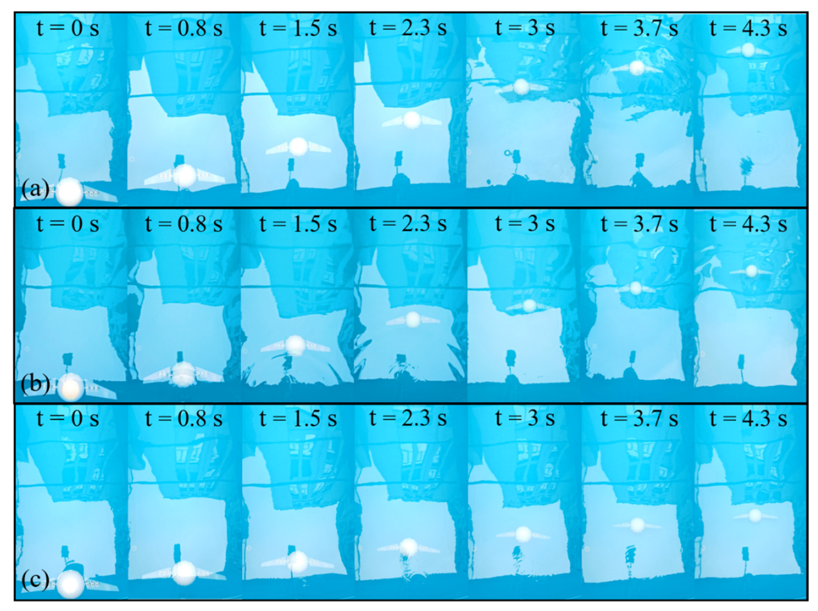
5.1. Experiment Results of Argo Mode

Figure 12 shows the two motion processes of the prototype in Argo mode for diving and climbing. During the experiment, the wings were vertically erected and the wing rotation angle was maintained at about 90°. The mobile buoy dives vertically into the water under the gravity and steadily approaches the bottom (see Figure 12a). It then climbs vertically due to buoyancy and progressively moves toward the water surface (see Figure 12b). Throughout the experiment, the prototype can smoothly complete the vertical profile movement and maintain the stability of the fuselage. The horizontal displacement of the mobile buoy is almost negligible, which is consistent with the dynamic simulation results (see Figure 9f) and proves the feasibility of the proposed mobile buoy moving in Argo mode.

5.2. Experiment Results of Glider Mode

Figure 13 and Figure 14 show time-stamped photographic sequences of the mobile buoy prototype in Glider mode during the diving phase and climbing phase with different wing rotation angles, respectively. As can be seen in Figure 13, the final glide distance of the mobile buoy decreases with the increase in the wing rotation angle for a constant dive depth. A similar trend is observed in Figure 14 during the climbing phase, which coincides with the relevant dynamic responses (see Figure 10h). Different wing rotation angles generate different lift and drag forces, thus affecting the gliding performance of the mobile buoy. The experimental results show that the wing rotation angle can adjust the mobile buoy to achieve a diving motion or climbing motion with different gliding attitudes.

Figure 15 and Figure 16 show time-stamped photographic sequences of the mobile buoy prototype during the diving phase and climbing phase with different net buoyancy mass, respectively, demonstrating the actual gliding trajectories. From the experimental results, it can be found that the larger the net buoyancy mass, the further the prototype glides at the same moment, i.e., the faster the mobile buoy glides. Typically, the greater the net buoyancy, the greater the lift of the mobile buoy, the faster it moves and the longer the glide distance under the same conditions. Despite the gliding velocity is different, the final gliding distance is roughly the same when the diving depth is the same. The net buoyancy mass has a relatively little effect on the gliding trajectory of the mobile buoy. However, a larger net buoyancy provides greater propulsion to propel the mobile buoy forward. The fundamental experiments verified the stability and feasibility of the mobile buoy in Glider mode, and demonstrated that the net buoyancy mass and the wing rotation angle are two key factors affecting the mobile buoy’s gliding performance.

6. Conclusions and Future Work

In this study, a novel mobile buoy is proposed, which has both vertical profiling kinematics similar to Argo profiling buoys and sawtooth gliding kinematics similar to underwater gliders by adjusting the wing rotation angle and net buoyancy mass. Considering the interplay between the mobile buoy and the fluid, a fluid–multibody coupled model is developed to analyze the dynamic response. Numerical simulation results demonstrate the ability of the proposed mobile buoy to perform vertical profile movements and sawtooth gliding motions. Based on the above theoretical analysis, a scaled-down prototype of the mobile buoy was fabricated and fundamental experiments were conducted to investigate the performance of the two motion modes. The experimental results show good agreement with the numerical simulation, proving the feasibility of the proposed mobile buoy concept and fluid–multibody coupled analysis method.

Although current research provides preliminary evidence of the feasibility of the mobile buoy, much remains to be carried out to make the mobile buoy practical for ocean observation. In the future, more attention needs to be paid to the optimization of the prototype and the design and improvement of hardware, such as battery packs, control systems and buoyancy regulation systems, enabling the achievement of stable motion mode switching during its underwater navigation. Sensors on the mobile buoy should also be explored and experiments in larger tanks should be conducted to more accurately monitor their energy consumption and movement. In addition, more elaborate hydrodynamic analysis of the mobile buoy, especially the wings and airfoil, is needed to optimize the design and improve the endurance of the mobile buoy.

References

1. Yuan, S.; Li, Y.; Bao, F.; Xu, H.; Yang, Y.; Yan, Q.; Zhong, S.; Yin, H.; Xu, J.; Huang, Z. Marine environmental monitoring with unmanned vehicle platforms: Present applications and future prospects. Sci. Total Environ. 2023, 858, 159741. [Google Scholar] [CrossRef] [PubMed]
2. Verfuss, U.K.; Aniceto, A.S.; Harris, D.V.; Gillespie, D.; Fielding, S.; Jiménez, G.; Johnston, P.; Sinclair, R.R.; Sivertsen, A.; Solbø, S.A. A review of unmanned vehicles for the detection and monitoring of marine fauna. Mar. Pollut. Bull. 2019, 140, 17–29. [Google Scholar] [CrossRef]
3. Jones, D.C.; Holt, H.J.; Meijers, A.J.; Shuckburgh, E. Unsupervised clustering of Southern Ocean Argo float temperature profiles. J. Geophys. Res. Ocean. 2019, 124, 390–402. [Google Scholar] [CrossRef]
4. Haavisto, N.; Tuomi, L.; Roiha, P.; Siiriä, S.-M.; Alenius, P.; Purokoski, T. Argo floats as a novel part of the monitoring the hydrography of the Bothnian Sea. Front. Mar. Sci. 2018, 5, 324. [Google Scholar] [CrossRef]
5. Xue, G.; Liu, Y.; Si, W.; Ji, C.; Guo, F.; Li, Z. Energy recovery and conservation utilizing seawater pressure in the working process of Deep-Argo profiling float. Energy 2020, 195, 116845. [Google Scholar] [CrossRef]
6. Cao, J.; Lu, D.; Li, D.; Zeng, Z.; Yao, B.; Lian, L. Smartfloat: A multimodal underwater vehicle combining float and glider capabilities. IEEE Access 2019, 7, 77825–77838. [Google Scholar] [CrossRef]
7. Orton, P.; McGillis, W.; Moisan, J.; Higinbotham, J.; Schirtzinger, C. The mobile buoy: An autonomous surface vehicle for integrated ocean-atmosphere studies. In AGU Spring Meeting Abstracts; ADS: Cambridge, MA, USA, 2009; p. OS22A–08. [Google Scholar]
8. Zoss, B.M.; Mateo, D.; Kuan, Y.K.; Tokić, G.; Chamanbaz, M.; Goh, L.; Vallegra, F.; Bouffanais, R.; Yue, D.K. Distributed system of autonomous buoys for scalable deployment and monitoring of large waterbodies. Auton. Robots 2018, 42, 1669–1689. [Google Scholar] [CrossRef]
9. Senga, H.; Kato, N.; Suzuki, H.; Yoshie, M.; Fujita, I.; Tanaka, T.; Matsuzaki, Y. Development of a new spilled oil tracking autonomous buoy. Mar. Technol. Soc. J. 2011, 45, 43–51. [Google Scholar] [CrossRef]
10. Senga, H.; Kato, N.; Suzuki, H.; Akamatsu, T.; Yu, L.; Yoshie, M.; Tanaka, T. Field experiments and new design of a spilled oil tracking autonomous buoy. J. Mar. Sci. Technol. 2014, 19, 90–102. [Google Scholar] [CrossRef]
11. Yu, F.; Hu, X.; Dong, S.; Liu, G.; Zhao, Y.; Chen, G. Design of a low-cost oil spill tracking buoy. J. Mar. Sci. Technol. 2018, 23, 188–200. [Google Scholar] [CrossRef]
12. Fan, S.; Woolsey, C.A. Dynamics of underwater gliders in currents. Ocean. Eng. 2014, 84, 249–258. [Google Scholar] [CrossRef]
13. Wang, S.; Yang, M.; Niu, W.; Wang, Y.; Yang, S.; Zhang, L.; Deng, J. Multidisciplinary design optimization of underwater glider for improving endurance. Struct. Multidiscip. Optim. 2021, 63, 2835–2851. [Google Scholar] [CrossRef]
14. Orozco-Muñiz, J.P.; Salgado-Jimenez, T.; Rodriguez-Olivares, N.A. Underwater glider propulsion systems VBS part 1: VBS sizing and glider performance analysis. J. Mar. Sci. Eng. 2020, 8, 919. [Google Scholar] [CrossRef]
15. Riser, S.C.; Freeland, H.J.; Roemmich, D.; Wijffels, S.; Troisi, A.; Belbéoch, M.; Gilbert, D.; Xu, J.; Pouliquen, S.; Thresher, A. Fifteen years of ocean observations with the global Argo array. Nat. Clim. Change 2016, 6, 145–153. [Google Scholar] [CrossRef]
16. Roemmich, D.; Alford, M.H.; Claustre, H.; Johnson, K.; King, B.; Moum, J.; Oke, P.; Owens, W.B.; Pouliquen, S.; Purkey, S. On the future of Argo: A global, full-depth, multi-disciplinary array. Front. Mar. Sci. 2019, 6, 439. [Google Scholar] [CrossRef]
17. Johnson, K.; Coletti, L.; Jannasch, H.; Martz, T.; Swift, D.; Riser, S. Long-term observations of ocean biogeochemistry with nitrate and oxygen sensors in Apex profiling floats. In AGU Fall Meeting Abstracts; ADS: Cambridge, MA, USA, 2008; p. OS31A–1232. [Google Scholar]
18. André, X.; Moreau, B.; Le Reste, S. Argos-3 satellite communication system: Implementation on the arvor oceanographic profiling floats. J. Atmos. Ocean. Technol. 2015, 32, 1902–1914. [Google Scholar] [CrossRef]
19. Sherman, J.; Davis, R.E.; Owens, W.; Valdes, J. The autonomous underwater glider” Spray”. IEEE J. Ocean. Eng. 2001, 26, 437–446. [Google Scholar] [CrossRef]
20. Webb, D.C.; Simonetti, P.J.; Jones, C.P. SLOCUM: An underwater glider propelled by environmental energy. IEEE J. Ocean. Eng. 2001, 26, 447–452. [Google Scholar] [CrossRef]
21. Eriksen, C.C.; Osse, T.J.; Light, R.D.; Wen, T.; Lehman, T.W.; Sabin, P.L.; Ballard, J.W.; Chiodi, A.M. Seaglider: A long-range autonomous underwater vehicle for oceanographic research. IEEE J. Ocean. Eng. 2001, 26, 424–436. [Google Scholar] [CrossRef]
22. Yang, Y.; Xiao, Y.; Li, T. A survey of autonomous underwater vehicle formation: Performance, formation control, and communication capability. IEEE Commun. Surv. Tutor. 2021, 23, 815–841. [Google Scholar] [CrossRef]
23. Ma, X.; Wang, Y.; Li, S.; Niu, W.; Ma, W.; Luo, C.; Yang, S. Formation control of discrete-time nonlinear multi-glider systems for both leader–follower and no-leader scenarios under switching topology: Cases for a fleet consisting of a wave glider and multiple underwater gliders. Ocean. Eng. 2023, 276, 114003. [Google Scholar] [CrossRef]
24. Alvarez, A.; Garau, B.; Caiti, A. Combining networks of drifting profiling floats and gliders for adaptive sampling of the Ocean. In Proceedings of the 2007 IEEE International Conference on Robotics and Automation, Rome, Italy, 21 May 2007; pp. 157–162. [Google Scholar]
25. Cao, J.; Lin, R.; Yao, B.; Liu, C.; Zhang, X.; Lian, L. Modeling, Control and Experiments of a Novel Underwater Vehicle with Dual Operating Modes for Oceanographic Observation. J. Mar. Sci. Eng. 2022, 10, 921. [Google Scholar] [CrossRef]
26. Zhou, H.; Cao, J.; Fu, J.; Liu, C.; Wei, Z.; Yu, C.; Zeng, Z.; Yao, B.; Lian, L. Dynamic modeling and motion control of a novel conceptual multimodal for autonomous sampling. Ocean. Eng. 2021, 240, 109917. [Google Scholar] [CrossRef]
27. Liu, B.; Yang, Y.; Wang, S.; Liu, Y. A dual-modal unmanned vehicle propelled by marine energy: Design, stability analysis and sea trial. Ocean. Eng. 2022, 247, 110702. [Google Scholar] [CrossRef]
28. Yang, M.; Wang, Y.; Zhang, X.; Liang, Y.; Wang, C. Parameterized dynamic modeling and spiral motion pattern analysis for underwater gliders. IEEE J. Ocean. Eng. 2022, 48, 112–126. [Google Scholar] [CrossRef]
29. Wang, P.; Wang, X.; Wang, Y.; Niu, W.; Yang, S.; Sun, C.; Luo, C. Dynamics Modeling and Analysis of an Underwater Glider with Dual-Eccentric Attitude Regulating Mechanism Using Dual Quaternions. J. Mar. Sci. Eng. 2022, 11, 5. [Google Scholar] [CrossRef]
30. Yang, S.; Li, L.; Li, X.; Liang, F.; Zhang, X.; Sun, W. Dynamics Model of Buoy Unpowered Heave Considering Seawater Density. J. Coast. Res. 2020, 99, 439–446. [Google Scholar] [CrossRef]
31. Zhu, X.; Yoo, W.S. Dynamic analysis of a floating spherical buoy fastened by mooring cables. Ocean. Eng. 2016, 121, 462–471. [Google Scholar] [CrossRef]
32. Qin, D.; Huang, Q.; Pan, G.; Shi, Y.; Li, F.; Han, P. Numerical simulation of hydrodynamic and noise characteristics for a blended-wing-body underwater glider. Ocean. Eng. 2022, 252, 111056. [Google Scholar] [CrossRef]
33. Le, T.-L.; Hong, D.-T. Computational fluid dynamics study of the hydrodynamic characteristics of a torpedo-shaped underwater glider. Fluids 2021, 6, 252. [Google Scholar] [CrossRef]
34. Wang, H.; Chen, J.; Feng, Z.; Li, Y.; Deng, C.; Chang, Z. Dynamics analysis of underwater glider based on fluid-multibody coupling model. Ocean. Eng. 2023, 278, 114330. [Google Scholar] [CrossRef]
35. Grande, D.; Huang, L.; Harris, C.A.; Wu, P.; Thomas, G.; Anderlini, E. Open-source simulation of underwater gliders. In Proceedings of the OCEANS 2021: San Diego–Porto, San Diego, CA, USA, 20–23 September 2021; pp. 1–8. [Google Scholar]
36. Liu, T. Evolutionary understanding of airfoil lift. Adv. Aerodyn. 2021, 3, 37. [Google Scholar] [CrossRef]
Figure 1. Working scheme of the mobile buoy.
Jmse 12 00150 g001
Figure 2. Mobile buoy with controllable wings, showing (a) shape and structural design, (b) switching motion mode by controlling wing rotation angle.
Jmse 12 00150 g002
Figure 3. Analysis process of fluid–multibody coupling method.
Jmse 12 00150 g003
Figure 4. Coordinate frames of the mobile buoy.
Jmse 12 00150 g004
Figure 5. The mass distribution of the mobile buoy.
Jmse 12 00150 g005
Figure 6. Motion in the vertical plane of the mobile buoy during an operation cycle.
Jmse 12 00150 g006
Figure 7. The hydrodynamics model, showing (a) the 3D computational domain, (b) a zoom-in view of the flow field mesh in X-Y slice plane, (c) the surface mesh of the mobile buoy.
Jmse 12 00150 g007
Figure 8. Mesh independence verification, showing (a) forward velocity, (b) pitch angle.
Jmse 12 00150 g008
Figure 9. Dynamic responses in Argo mode, showing (a) forward velocity, (b) heave velocity, (c) pitch angle, (d) pitch moment, (e) angular velocity around the Y-axis direction and (f) motion trajectory.
Jmse 12 00150 g009
Figure 10. Dynamic responses under different wing rotation angles during the Glider mode, showing (a) forward velocity, (b) heave velocity, (c) angular velocity around the Y-axis direction (d) pitch angle, (e) force, (f) moment, (g) motion velocity and (h) motion trajectory.
Jmse 12 00150 g010
Figure 11. Dynamic responses under different net buoyancy masses during the Glider mode, showing (a) forward velocity, (b) heave velocity, (c) angular velocity around the Y-axis direction (d) pitch angle, (e) force, (f) moment, (g) motion velocity and (h) motion trajectory.
Jmse 12 00150 g011
Figure 12. Photographic sequences of motion process in Argo mode, showing (a) diving phase, (b) climbing phase.
Jmse 12 00150 g012
Figure 13. Photographic sequences of motion process in Glider mode with different wing rotation angles during diving phase, showing (a) αw = 30°, (b) αw = 40° and (c) αw = 50°.
Jmse 12 00150 g013
Figure 14. Photographic sequences of motion process in Glier mode with different wing rotation angles during climbing phase, showing (a) αw = 30°, (b) αw = 40° and (c) αw = 50°.
Jmse 12 00150 g014
Figure 15. Photographic sequences of motion process in Glider mode with different net buoyancy mass during diving phase, showing (a) m0 = 0.3, (b) m0 = 0.4 and (c) m0 = 0.5.
Jmse 12 00150 g015
Figure 16. Photographic sequences of motion process in Glider mode with different net buoyancy mass during climbing phase, showing (a) m0 = 0.3, (b) m0 = 0.4 and (c) m0 = 0.5.
Jmse 12 00150 g016