Dynamic Mechanical Properties and Damage Parameters of Marine Pipelines Based on Johnson–Cook Model

Abstract

A comprehensive understanding of the dynamic behavior of materials and structures under impact loads is paramount for the design and maintenance of reliable marine pipelines and associated structures. However, there is a lack of comprehensive research on the full characterization of constitutive and failure models of carbon steels, which are commonly used in marine pipelines. In this paper, Q235 steel was subjected to quasi-static tensile tests at room temperature on smooth specimens to obtain the constitutive parameters using the Johnson–Cook (J-C) model. Subsequently, quasi-static tensile tests were conducted on notched specimens, and dynamic tensile tests were performed on smooth round bars to obtain stress triaxiality and failure strain. The acquired data were then utilized to fit the failure parameters using the Johnson–Cook (J-C) damage model, a widely accepted constitutive model employed in high-strain rate applications through the least squares method. Finally, the tensile test is numerically simulated based on the acquired experimental parameters. The obtained results reveal a remarkable agreement between the curve fitted by the J-C constitutive model and the experimental tensile curve. Additionally, a high degree of correlation between the load-displacement curves of the tests and simulations provides robust validation of the accuracy of the dynamic mechanical parameters for Q235 steel. These findings contribute valuable insights into the behavior of carbon steels commonly used in marine pipelines, enhancing the overall understanding of their response to impact loads and informing more reliable design and maintenance practices.

1. Introduction

The exploitation and utilization of marine oil and gas resources are of utmost importance for a country’s energy supply. Marine pipelines play a critical role as essential conduits for transporting these valuable marine resources. The marine environment presents numerous challenges, as pipelines are exposed to potential impacts from a range of sources, including natural disasters such as tsunamis, storm surges, and earthquakes, as well as human activities like falling objects and trawling [1,2]. Consequently, subsea pipelines and thin-walled metal structures undergo high-speed, dynamic processes that result in significant deformation [3,4]. When subjected to impact loads, these structures are susceptible to local dents and cracking damages, posing direct threats to the safety and reliability of the pipelines. In severe cases, such damage can lead to pipeline leakage and explosion accidents. Therefore, comprehensive research on the dynamic mechanical properties of these structures is essential to accurately characterize material failure behavior, thereby enhancing their overall safety and performance.

Ellinas [5] proposed a semiempirical formula for plastic damage at the impact point of a pipeline due to impact loads, drawing from classical ultimate plasticity theory. However, they omitted consideration of the pipeline’s contact with the seabed. Wierzbick et al. [6] explored the influence of initial axial force, providing empirical formulas for dent depth and absorbed energy, alongside impact force formulas that overlooked shear force conditions. Bai [7] examined the mutual contact between falling objects and the pipeline, presenting a semiempirical formula for impact loads and damage depth at the impact point. Wang et al. [8] delved into energy conversion during the impact of falling objects on marine pipelines but overlooked the seabed’s influence on energy. DNV synthesized prior research, creating regulations for marine pipeline damage from impact loads and offering a formula to calculate dent depth caused by falling object impacts [9,10]. Nonetheless, this formula disregarded the impact process’s nonlinear aspects and failed to consider energy absorption by the seabed, falling objects, and backfill soil above the pipeline. Theoretical analysis can yield straightforward calculation formulas, but their limitations prevent them from comprehensively addressing real-world situations, resulting in notable deviations in calculations. Chen et al. [11] utilized hammer impact experiments to explore how internal pressure affects marine pipeline impact damage. They found that internal pressure can partly suppress pipeline deformation but may also lead to overall pipeline failure. Notably, these experiments did not account for the effects of seawater and the seabed on the pipeline. Building upon this work, Andrew [12,13] enhanced the experiments by incorporating the influence of concrete protective layers and soil. They established a correlation between dent depth, impact energy from falling objects, and energy absorbed by the pipeline. Summarizing common pipeline impact tests across diverse fields, Zhang [14] designed experimental setups for lateral and vertical hammer impacts on pipelines. Given the costliness of impact experiments, contemporary research predominantly relies on numerical simulation methods to examine the process of falling object impacts on marine pipelines. This approach can address nonlinear concerns between various objects and visually depict the entire impact process, producing similarly accurate outcomes. Taking into consideration the interaction between the seabed and the pipeline, Zeinoddini [15] conducted a comparative analysis of experiments and numerical simulations. This analysis explored variations in impact force, displacement, dent depth, and energy for an X70 pipeline under distinct conditions, including different impact models and internal pressures. Yan [16] delved into the damage caused to marine pipelines by objects dropped from platforms or supply ships. They introduced a simple and feasible method to study the effects of pipeline damage under impact loads. In a similar vein, Huang [17] conducted marine pipeline damage experiments and numerical simulations. Their study examined the influence of falling object mass, height, and shape on mechanical damage to marine pipelines, and they adjusted the Ellinas–Walker formula based on experimental findings.

The impact on marine pipelines involves a rapid deformation and damage process. The material’s constitutive relationship differs markedly from static scenarios. The majority of the aforementioned studies gauge damage based on the extent of macroscopic pipeline deformation, disregarding material damage attributed to strain rate effects. Further research is warranted to investigate the dynamic mechanical properties of pipeline materials.

In the research of material dynamic mechanical properties, the application of the Hopkinson bar has become relatively mature. The Hopkinson Bar Tensile Test involves applying a sudden impact or stress wave to a specimen to induce tensile stress. The stress wave is generated by impacting the input bar (also called the striker bar) with a projectile, which then travels through the bar and the specimen. The stress wave’s characteristics, such as its amplitude, duration, and velocity, are monitored and used to calculate the mechanical properties of the material. It allows testing at strain rates in the range of 10² to 10⁴ s⁻¹. Within this range, establishing an appropriate constitutive model can predict the true stress–strain relationship of materials under high strain rates. Commonly used constitutive models include the Johnson–Cook (J-C) model, the Zerilli–Armstrong model, the Steinberg model, etc. Among these, the J-C model is widely adopted by many researchers due to its ability to consider the combined effects of stress state, strain rate, and temperature on material failure. The model is known for its simple form, making its parameters easy to test and calibrate [18,19,20,21]. Additionally, the Johnson–Cook model is often integrated into finite element simulation software to predict the behavior of metals during forming processes, such as forging, stamping, rolling, and extrusion.

Previous research on the dynamic impact response of metals has predominantly centered on the use of alloy materials. Through a combination of experiments and numerical simulations, researchers have determined parameters for the J-C model, while also evaluating the validity of the J-C constitutive relationship and failure criteria [22,23,24,25,26,27,28]. However, marine pipelines are primarily made of carbon steel. Wei et al. studied the mechanical behavior of quenched and tempered 45# steel at temperatures ranging from room temperature to 1000 °C and strain rates from 10⁻⁴ to 10³ s⁻¹. They calibrated the model parameters by combining the back-calculation of critical cracking from Taylor impact tests [29]. Zhu et al. conducted experiments and numerical simulations on Q355B steel, determining 10 parameters for the J-C model [30]. However, Q355B steel is commonly used in construction engineering applications. Some scholars have also studied the impact resistance of Q235 steel [31,32,33], but they did not provide all the parameters for the constitutive and failure models. Moreover, they did not validate the accuracy of the experimental results. The comprehensive evaluation of the precision exhibited by the J-C constitutive model encountered inherent complexities stemming from two distinct rationales. First, the deficiency in an exhaustive set of test data pertaining to a designated material across varied loading circumstances, encompassing authentic stress-authentic strain interdependencies, ramifications of strain-rate variations, temperature fluctuations, and structural failure mechanisms, engendered impediments to a holistic assessment. Second, the cost would be prohibitively high if a complete set of the test data were obtained.

Therefore, this paper employs a universal material testing machine and the Hopkinson bar (SHTB) experimental system to comprehensively investigate the quasi-static and dynamic tensile properties of Q235 steel commonly used for marine pipelines at room temperature. Based on the J-C model, the parameters are determined. Furthermore, numerical simulations are conducted to validate the accuracy of the J-C model, providing valuable reference for the impact dynamic design and damage assessment of marine pipelines. The main variable parameters in this study are summarized in

Table 1. Nomenclature.

Parameters	Description
$\sigma$	The equivalent stress
${\sigma }^{\prime }$	The engineering stress
${\sigma }_m$	The average stress
${\sigma }_1$, ${\sigma }_2$, ${\sigma }_3$	The principal stresses
${\sigma }^{*}$	the stress triaxiality
$\epsilon$	The equivalent strain
${\epsilon }^{\prime }$	The engineering strain
$\dot{\epsilon }$	The strain rate
$\dot{{\epsilon }_0}$	The reference strain rate
${\epsilon }^{*}$	Dimensionless strain rate
${\epsilon }_f$	The effective fracture strain
$A$	The yield stress of the material
$B$, $n$	The strain hardening constants
$C$	The strain-rate strengthening coefficient
$D_1$, $D_2$, $D_3$, $D_4$	Material damage parameters

.

2. Constitutive Model and Damage Model

2.1. Johnson–Cook Constitutive Model

The J-C constitutive relation is shown in Equation (1) [34,35],

$$\sigma =\left(A+B{\epsilon }^n\right)\left(1+C\ln \frac{\dot{\epsilon }}{\dot{{\epsilon }_0}}\right)\left[1-{\left(\frac{T-T_{room}}{T_{melt}-T_{room}}\right)}^m\right]$$

(1)

where $\sigma$ is the equivalent stress, $\epsilon$ is the equivalent strain, $A$ is the yield stress of the material, $B$ and $n$ are the strain hardening constants, $C$ is the strain-rate strengthening coefficient, ${\epsilon }^{*}=\frac{\dot{\epsilon }}{\dot{{\epsilon }_0}}$ is dimensionless strain rate, $\dot{{\epsilon }_0}$ is the reference strain rate, $m$ is the temperature softening coefficient, and $T_{room}$ and $T_{melt}$ are the room temperature and the melting point of the material, respectively.

The J-C constitutive model comprises three fundamental components that account for the material’s response to strain hardening, strain-rate strengthening, and temperature softening, significantly influencing the flow stress. In situations where the impact of temperature remains negligible, the third term representing temperature softening can be omitted, resulting in a simplified form of the constitutive model, as shown in Equation (2).

$$\sigma =\left(A+B{\epsilon }^n\right)\left(1+C\ln {\epsilon }^{*}\right)$$

(2)

The parameters $A$, $B$, and $n$ can be determined by conducting quasi-static tensile tests on smooth round bars at a reference strain rate and a reference temperature. In this case, the equation simplifies to Equation (3).

$$\sigma =A+B{\epsilon }^n$$

(3)

During the tensile process of the specimen, the stress corresponding to the initial yield point of the material is donated as $A$. Taking the logarithm of both sides of Equation (3), we have:

$$\ln \left(\sigma -A\right)=\ln B+n\ln \epsilon$$

(4)

By performing linear regression on $\ln \left(\sigma -A\right)$ − $\ln \epsilon$ curves, the slope and intercept values can be determined, which correspond to the $n$ and $B$, respectively.

Conduct tensile tests at varying strain rates to explore the relationship between the stress and strain rate. At each strain rate, measure the stress values at a consistent strain level to examine their correlation. The correlation between stress and strain rates at a given strain level is mathematically described by Equation (5), offering valuable insights into the material’s behavior under different loading conditions.

$$\sigma =C\ln {\epsilon }^{*}+\mathrm{c}\mathrm{o}\mathrm{n}\mathrm{s}\mathrm{t}\mathrm{a}\mathrm{n}\mathrm{t}$$

(5)

Next, plot the stress values against the natural logarithm of the strain rate for each fixed strain level. By analyzing these data, the strain-rate sensitivity constant, denoted as $C$, can be precisely determined.

2.2. Johnson–Cook Damage Model

J-C damage model proposes that as the number of time steps increases, the plastic strain of the material accumulates. When the accumulated plastic strain reaches the fracture strain of the material, the damage value becomes 1, indicating failure of the material, as shown in Equation (6).

$$D=\sum \frac{∆{\epsilon }_p}{{\epsilon }_f}$$

(6)

where, $∆{\epsilon }_p$ represents the equivalent plastic strain increment, and ${\epsilon }_f$ represents the effective fracture strain at the current time step. The effective fracture strain is determined by the stress state, strain rate, and temperature, and its expression is given by Equation (7) [34,35].

$${\epsilon }_f=\left(D_1+D_2{e}^{D_3\frac{{\sigma }_m}{\sigma }}\right)\left(1+D_4\ln {\epsilon }^{*}\right)\left[1+D_5\left(\frac{T-T_{room}}{T_{melt}-T_{room}}\right)\right]$$

(7)

where, $D_1$ to $D_5$ are material damage parameters, ${\sigma }^{*}=\frac{{\sigma }_m}{\sigma }$ represents the stress triaxiality, ${\sigma }_m$ is the average stress, and $\sigma$ is the equivalent stress, which is calculated as follows:

$${\sigma }_m=\frac{1}{3}\left({\sigma }_1+{\sigma }_2+{\sigma }_3\right)$$

(8)

$$\sigma =\sqrt{\frac{1}{2}\left[{\left({\sigma }_1-{\sigma }_2\right)}^2+{\left({\sigma }_2-{\sigma }_3\right)}^2+{\left({\sigma }_1-{\sigma }_3\right)}^2\right]}$$

(9)

In the above equations, ${\sigma }_1$, ${\sigma }_2$, and ${\sigma }_3$ are the principal stresses.

The J-C damage model is also composed of three parts, which represent the influence of stress triaxiality, strain rate, and temperature on the material’s failure strain, respectively. When the effect of temperature is not considered, Equation (7) can be simplified to:

$${\epsilon }_f=\left(D_1+D_2{e}^{D_3{\sigma }^{*}}\right)\left(1+D_4\ln {\epsilon }^{*}\right)$$

(10)

At the reference strain rate, the relationship between failure strain and stress triaxiality becomes:

$${\epsilon }_f=D_1+D_2{e}^{D_3{\sigma }^{*}}$$

(11)

Conduct tensile tests at different strain rates and use the method of least squares to fit the data, the values of parameters $D_1$ to $D_3$ can be determined. Furthermore, at the same stress state, the material’s failure strain is linearly related to the natural logarithm of the relative strain rate, and the slope of this linear relationship gives the value of parameter $D_4$.

3. Mechanical Properties Tests of the Material

3.1. Tested Material

For this study, Q235 steel is chosen as the test material due to its widespread application in marine oil and gas pipelines. The specimens utilized in this investigation are sourced from a uniform 15 mm-diameter Q235 steel rod, with its primary chemical composition detailed in

Table 2. Main chemical composition of Q235 steel.

C/%	Si/%	Mn/%	P/%	S/%
0.16	0.12	0.38	0.023	0.040

.

Given the virtual absence of the phenomenon of temperature-induced material softening within marine environments, the present study is prominently centered upon the material’s response under distinct strain rates, with an exclusion of temperature effects from the analytical purview. Therefore, the determination of the eight common parameters in Equations (2) and (10) is deemed adequate for characterizing the material’s constitutive relationship and failure strain.

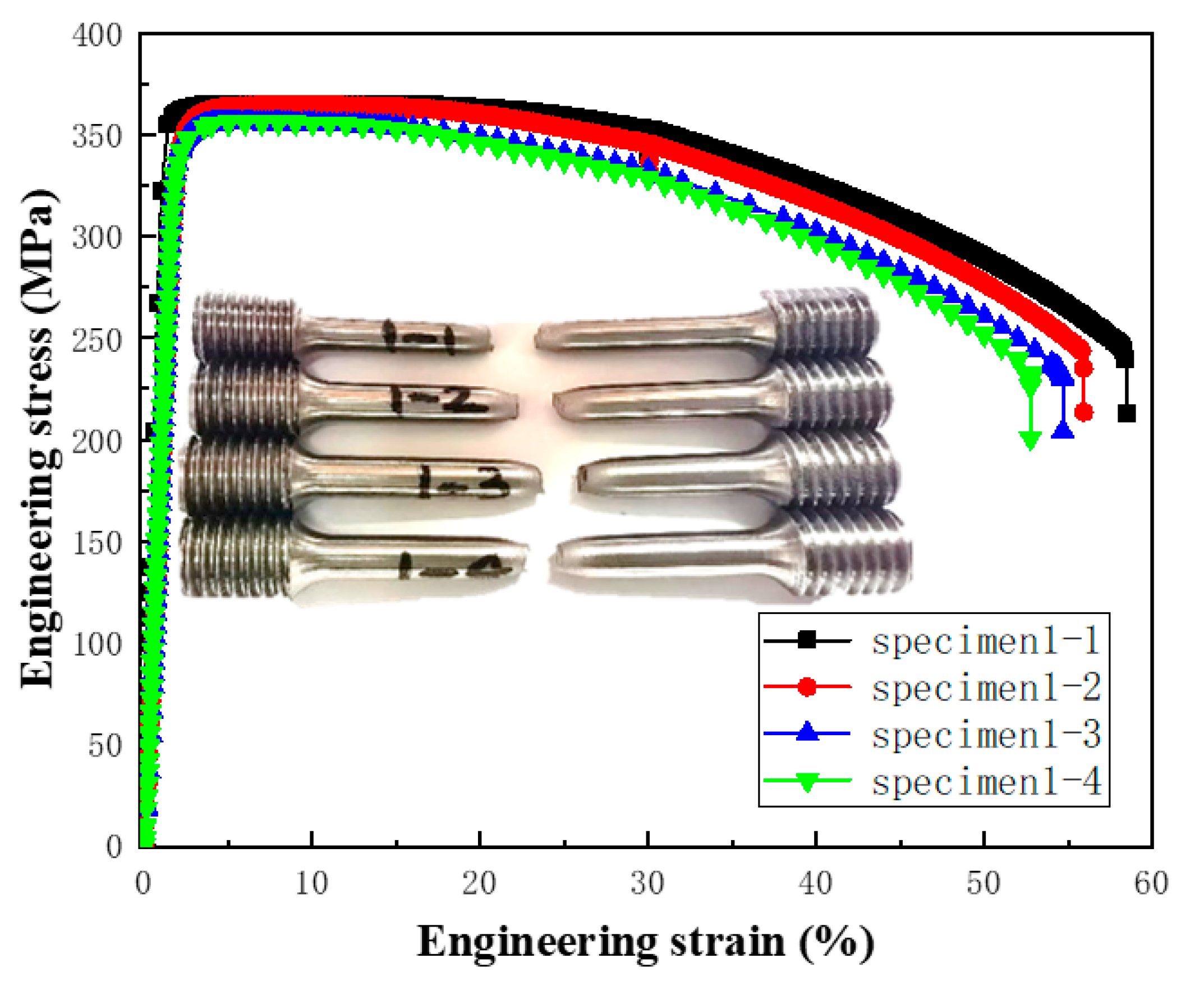
3.2. Quasi-Static Tensile Tests of Smooth Specimens

A series of quasi-static tensile tests were designed using smooth specimens. The detailed dimensions of the test specimens are illustrated in Figure 1. Two distinct strain rates, 0.001 s⁻¹ and 0.0001 s⁻¹, were selected to assess the material’s response under varying loading conditions. To ensure data accuracy and validation, two sets of tensile tests were conducted at each strain rate, with specimen numbers designated as 1–1 to 1–4 (specimens 1–2 and 1–4 are served as control tests).

Loads and displacements were recorded and calculated to derive the engineering stress–strain curves of Q235 steel, as presented in Figure 2.

The conventional nominal stress–strain curve, commonly employed in engineering contexts, possesses limitations in accurately portraying the complete constitutive behavior of steel as it undergoes plastic deformation phases. To achieve a more faithful representation of the material’s plastic deformation response under tensile loading, it becomes imperative to employ the true stress–strain curve. This true curve can be derived through the transformation of the engineering stress–strain curve, executed prior to the onset of necking within the specimen. The mathematical transformations, as expressed in Equations (12) and (13) [3], facilitate the derivation of said true stress–strain curve.

$$\sigma ={\sigma }^{\prime }\left(1+{\epsilon }^{\prime }\right)$$

(12)

$$\epsilon =\ln \left(1+{\epsilon }^{\prime }\right)$$

(13)

where, ${\sigma }^{\prime }$ and $\sigma$ are engineering stress and true stress, respectively, and ${\epsilon }^{\prime }$ and $\epsilon$ are engineering strain and true strain, respectively.

The morphology of the four fractured specimens is visually depicted in the figure, offering key insights into the fracture behavior of Q235 steel under quasi-static tensile conditions. Remarkably, fracture initiation predominantly occurred at the center of each specimen, resulting in distinct necking observed in the fracture region. The reduction of the area for specimens 1–1 to 1–4 were calculated using Equation (14) as follows: 58.53%, 56.51%, 56.31%, and 54.64%, respectively. In this equation, $A_0$ and $A_f$ denote the cross-sectional areas of the gauge section before and after the specimen’s fracture, respectively. Furthermore, the fracture surfaces exhibit a distinct 45-degree angle, offering compelling evidence of substantial plastic deformation during the tensile tests. The Elastic Modulus of Q235 steel was determined to be 200 GPa, and the average yield strength was precisely measured at 361.2 MPa, corresponding to the value of parameter $A$ in the J-C constitutive model.

$$\psi =\frac{A_0-A_f}{A_0}$$

(14)

A comprehensive fitting analysis was performed to establish the relationship between $\ln \left(\sigma -A\right)$ and $\ln \epsilon$, as illustrated in Figure 3. The fitting procedure yielded two essential parameters, $B$ = 526 MPa and $n$ = 0.58, characterizing the material’s response under quasi-static tensile conditions.

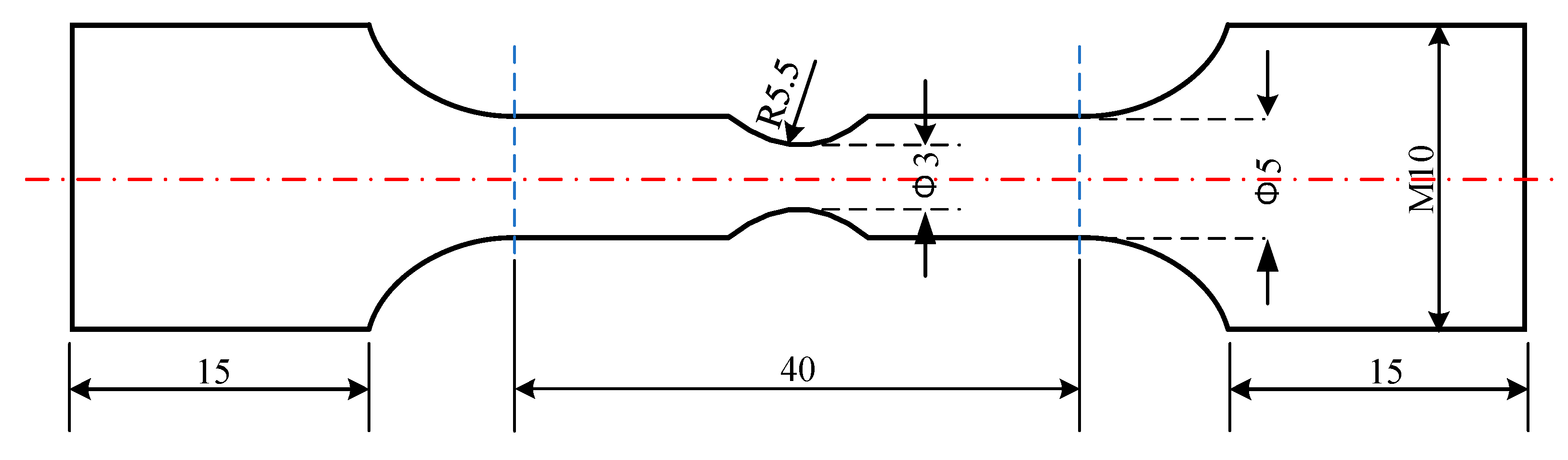
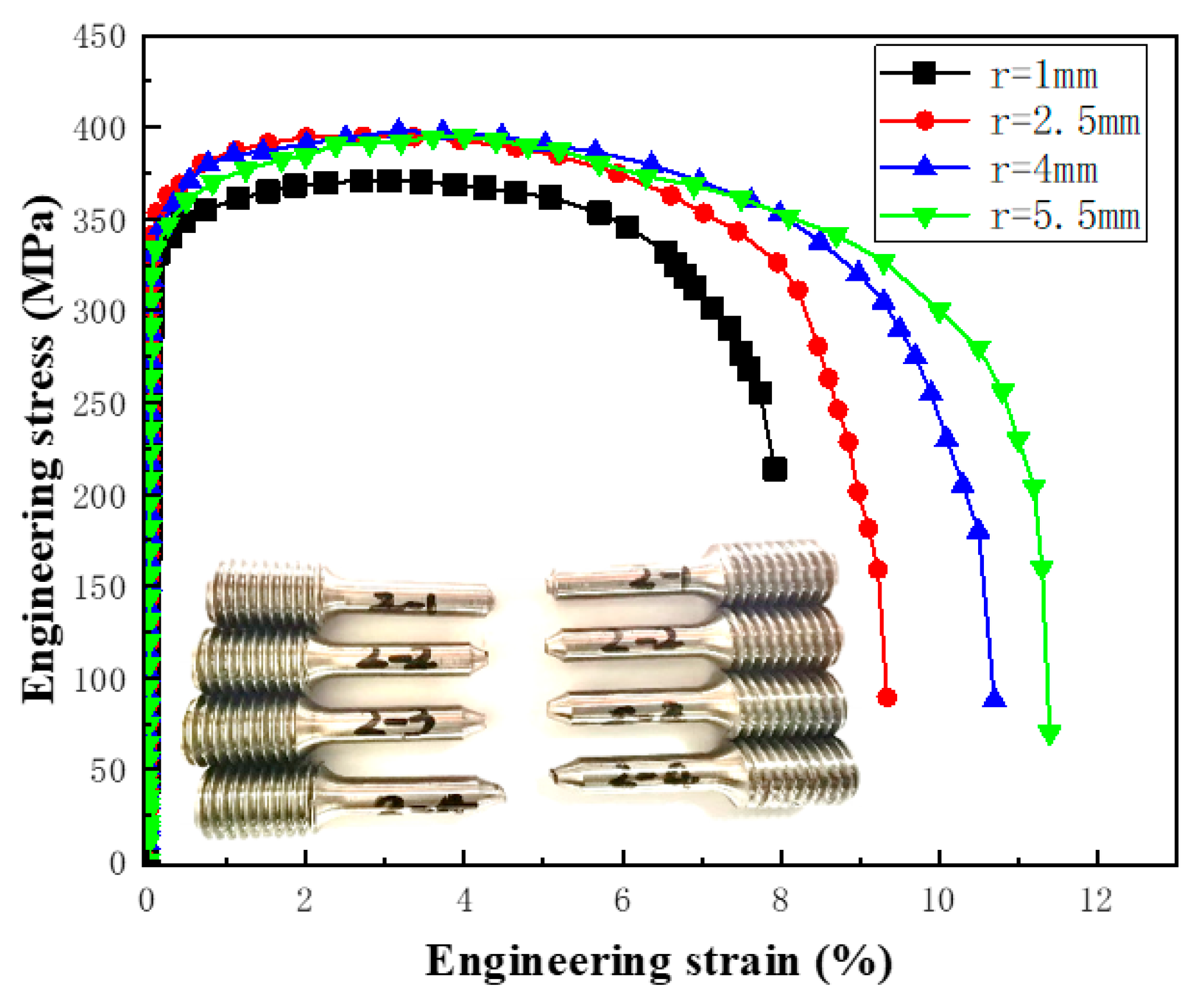
3.3. Tensile Tests of Notched Specimens

Tensile tests were conducted on specimens with different notch radii at the rod center to investigate the material’s behavior under various stress states. To obtain different stress triaxialities, four different notch radii were designed: 1 mm, 2.5 mm, 4 mm, and 5.5 mm, covering a wide range of stress states. The dimensions of the specimens are shown in Figure 4. The specimens were numbered as 2–1 to 2–8, with specimens 2–5 to 2–8 designated as control tests for comparative analysis. A constant tensile strain rate of 0.001 s⁻¹ was selected for all tests to ensure consistency and accuracy in the experimental setup.

Figure 5 presents the stress–strain curves of specimens with different notch radii. With increasing notch radius, the material exhibits improved plastic behavior.

In the tensile tests of smooth specimens, the stress triaxiality is −1/3. However, for the tensile tests of notched specimens, the stress triaxiality can be calculated by Equation (15):

$${\sigma }^{*}=-\frac{1}{3}-\ln \left(1+\frac{a}{2R}\right)$$

(15)

where, $a$ is the specimen radius, and $R$ is the notch radius.

Figure 6 presents the data of failure strain for different stress triaxiality conditions. The tensile tests results are shown in

Table 3. Tensile test results of notched specimens.

The Notch Radius /mm	Initial Specimen Diameter /mm	Specimen Diameter after Fracture /mm	The Initial Stress Triaxiality	The Stress Triaxiality after Fracture	Reduction of Area /%
1	3	2.55125	−0.8929	−0.8267	13.83
2.5	3	2.40375	−0.5957	−0.5487	17.89
4	3	2.2975	−0.5052	−0.4675	20.66
5.5	3	2.16875	−0.4612	−0.4274	23.85

. In quasi-static tensile tests, failure strain decreases as the stress triaxiality increases. Based on the data presented in Figure 6, a fitting analysis was performed using Equation (11) to determine the parameters $D_1$ to $D_3$, with values of $D_1$ = 0.2918, $D_2$ = 4.6156, and $D_3$ = 6.1566.

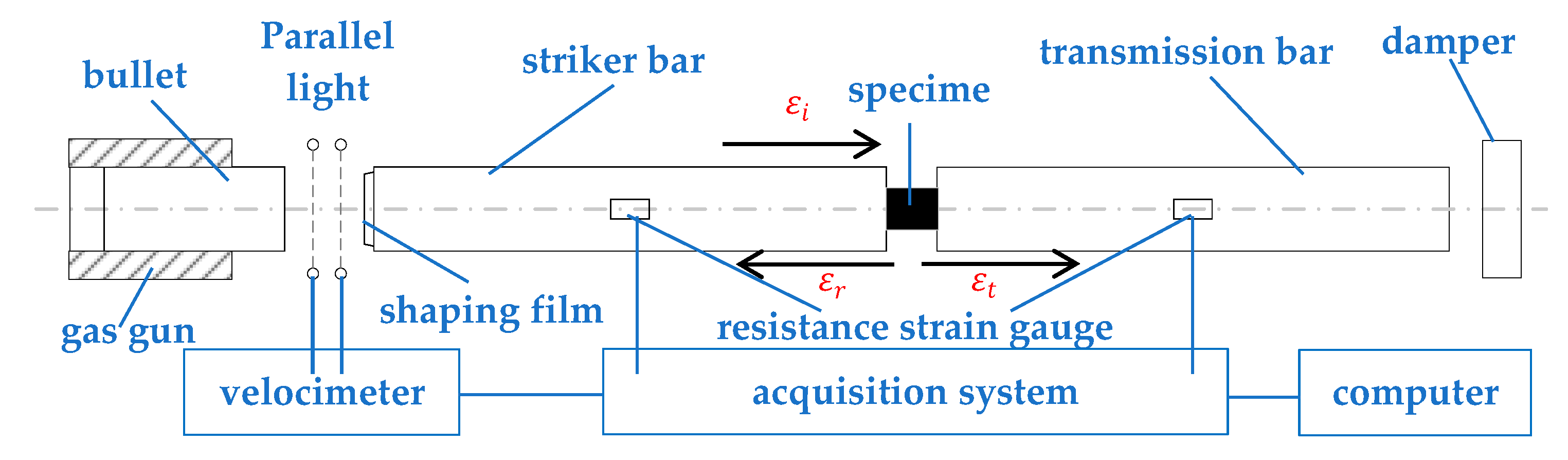
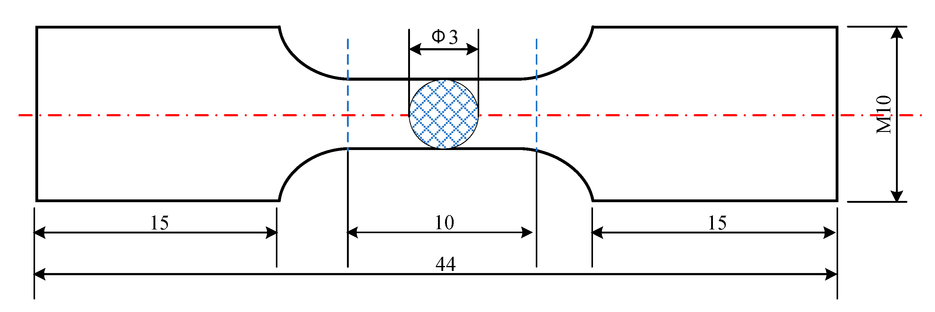
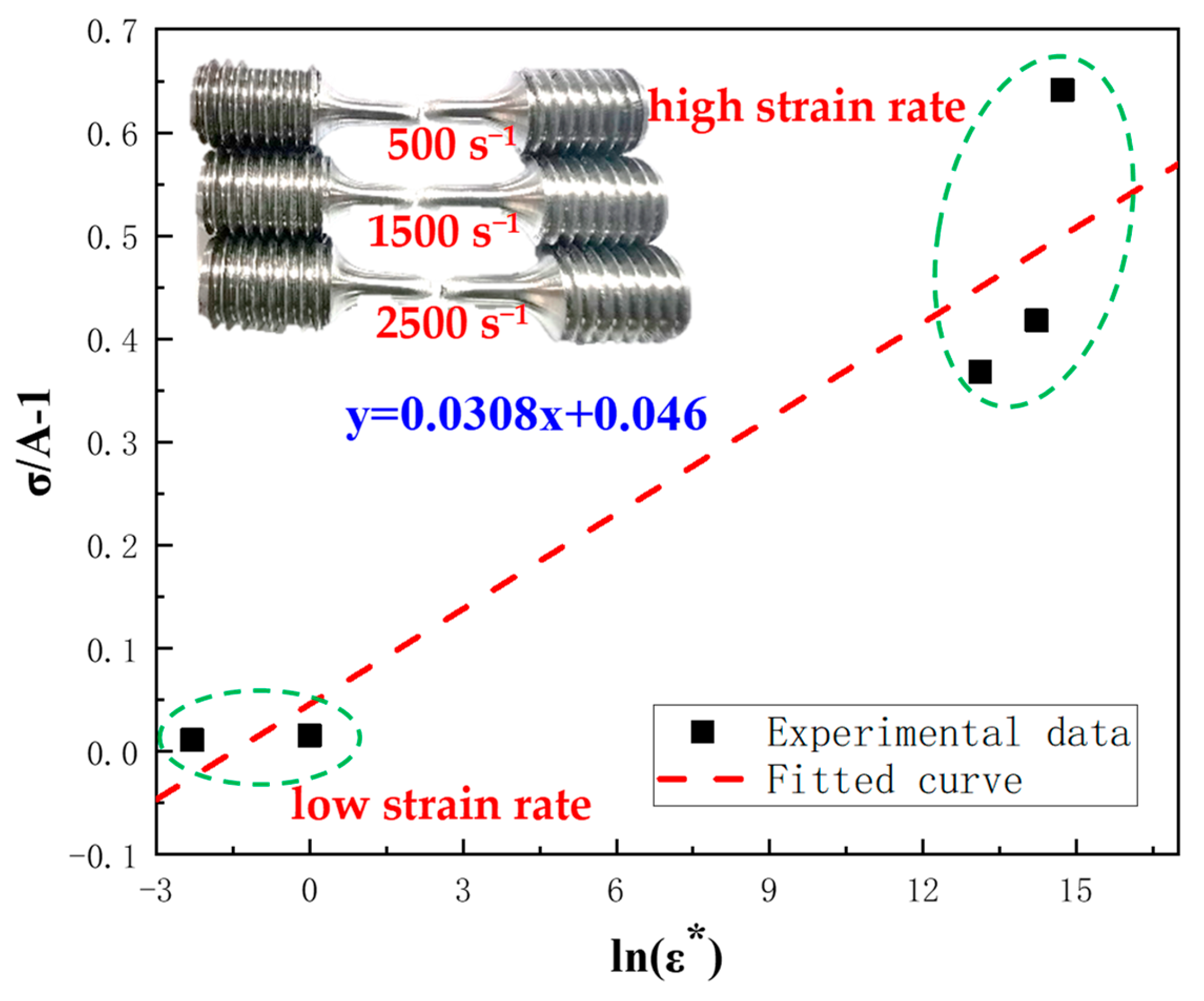
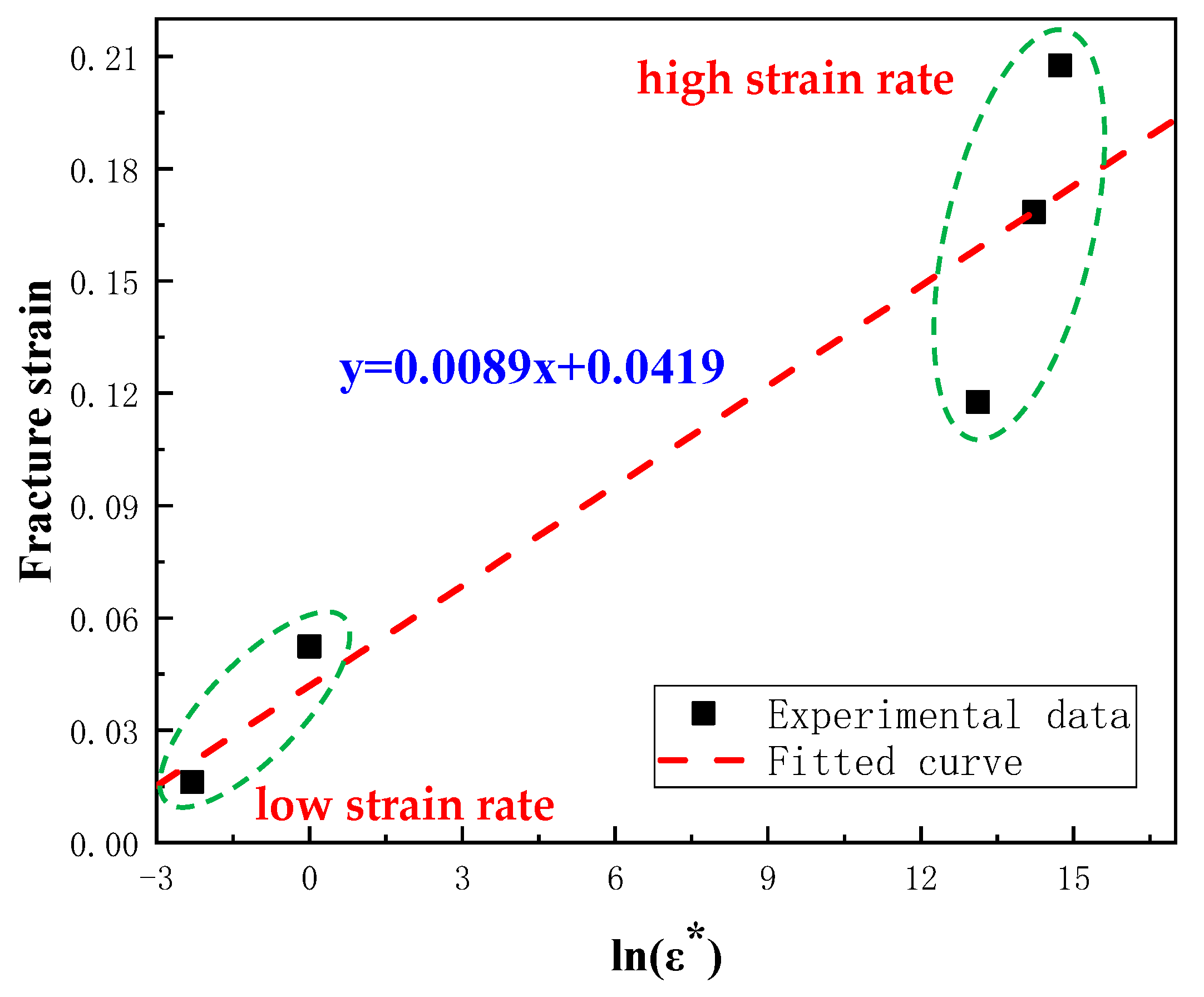
3.4. Hopkinson Tensile Test at Different Strain Rates

The split Hopkinson bar test is a widely employed technique for investigating the dynamic mechanical properties of metal materials, particularly their dynamic tensile behavior, at high strain rates. This versatile test method encompasses a broad strain-rate range, typically spanning from 10² to 10⁴ s⁻¹, enabling comprehensive analyses of material response under dynamic loading conditions. Through the measurement of stress–strain curves at various strain rates, this experiment aims to obtain the fundamental parameters required for the J-C material model.

To comprehensively characterize the dynamic tensile properties of Q235 steel, Hopkinson dynamic tensile tests were performed at three distinct strain rates: 500 s⁻¹, 1500 s⁻¹, and 2500 s⁻¹. The experimental principle is shown in Figure 7.

The test setup consists of three main components: the striker bar (or input bar), the specimen, and the transmission bar (or output bar). The striker bar is a high-strength bar that is struck by a projectile (usually a gas gun) to generate the stress wave. It is in contact with the specimen. The test material is in the form of a thin cylinder or tube placed between the striker bar and the transmission bar. When the striker bar is impacted, it transmits a stress wave to the specimen, inducing tension. A fraction of the pulse propagates through the specimen, inducing rapid plastic deformation. Simultaneously, a portion of the pulse traverses the specimen, permeating the transmission bar, where it is subsequently dissipated by the buffering mechanism. Additionally, a residual fraction is retro-reflected back through the striker bar. The transmission bar transmits the stress wave to a set of strain gauges or other measuring devices. These strain gauges measure the deformation of the specimen under tension, such as the incident strain ${\epsilon }_i$, the reflection strain ${\epsilon }_r$, and the transmission strain ${\epsilon }_t$. By analyzing the stress and strain data, the material’s dynamic tensile properties can be determined, such as stress–strain curves, strain-rate sensitivity, and fracture behavior at high strain rates.

The specimen dimensions are shown in Figure 8. Three distinct experimental series were conducted, encompassing a dual configuration wherein two series employed projectiles of 600 mm in length, subject to strain rates of 500 s⁻¹ and 1500 s⁻¹, respectively. Meanwhile, the third series featured a projectile of 400 mm length, subjected to a strain rate of 2500 s⁻¹. Notably, each experimental was repeated to ensure robustness of the results. Subsequent to data acquisition, the empirical findings were analyzed employing the venerable classical two-wave method as delineated in reference [36], culminating in the derivation of precise engineering stress–strain relationships. To counteract the potential influence stemming from transverse deformation of the specimens, Equations (12) and (13) were employed to effectuate a transformation of the recorded data, resulting in the extraction of true stress and strain manifestations.

At the reference strain rate $\dot{{\epsilon }_0}$ = 0.001 s⁻¹, the variation of Q235 steel’s equivalent stress and failure strain with the natural logarithm of the dimensionless strain rate $\ln {\epsilon }^{*}$ was plotted at a consistent plastic strain level. These plots are illustrated in Figure 9 and Figure 10, respectively. Our findings highlight the substantial influence of strain rate on Q235 steel’s equivalent stress and failure strain. Notably, the material displays distinct linear relationships at low and high strain rates. Particularly, at higher strain rates, the equivalent stress and failure strain exhibit heightened sensitivity to variations in strain rate.

Through fitting the equivalent stress and failure strain data at different strain rates, we successfully determined the values of the parameters $C$ and $D_4$, illustrated by the dashed lines in Figure 9 and Figure 10. The linear fitting outcomes revealed parameter values of $C$ = 0.0308 and $D_4$ = 0.0089.

4. Validation of the Johnson–Cook Constitutive Model and Failure Parameters through Numerical Simulations

4.1. The Finite Element Models

Finite element analysis (FEA) using the Johnson–Cook model enables the visualization of stress and strain distributions, as well as the prediction of potential defects like cracks or wrinkles. To validate the precision of the eight parameters proposed for the J-C constitutive model and failure model in the preceding section, numerical simulations of Q235 steel tensile tests were conducted.

A three-dimensional solid finite element model of the tensile specimen was developed, adhering to the dimensions as depicted in Figure 1. In the material property module, the Johnson–Cook strengthening model was chosen for plasticity, and the Johnson–Cook damage model was selected for ductile metal damage. The parameters are listed in

Table 4. J-C parameters of Q235 steel.

$\mathit{A}$	$\mathit{B}$	$\mathit{C}$	$\mathit{n}$	${\mathit{D}}_1$	${\mathit{D}}_2$	${\mathit{D}}_3$	${\mathit{D}}_4$
361.2 MPa	526 MPa	0.0308	0.58	0.2918	4.6156	6.1566	0.0089

, which were obtained from the tensile tests.

A failure displacement of 0.001 mm was set for damage evolution. The material density is 7850 kg/m³. Computational accuracy was ensured by setting the mesh size in the gauge section to 0.5 mm, with appropriate size increment in the grip section. The model comprised a total of 32,240 elements, as depicted in Figure 11.

Two reference points were set at the top and bottom ends of the specimen, respectively. Coupling constraints were applied between the reference points and the grip sections. While the bottom reference point was kept fixed, a controlled vertical upward velocity of 0.04 mm/s was applied to the top reference point.

To precisely determine the strain values, two reference points were selected on the gauge section of the model, as shown in Figure 11. The distance between the two points is 34 mm. Their displacements along the tensile direction were set in the History Output section. In addition, the reaction force of the top reference point was also output in the vertical direction.

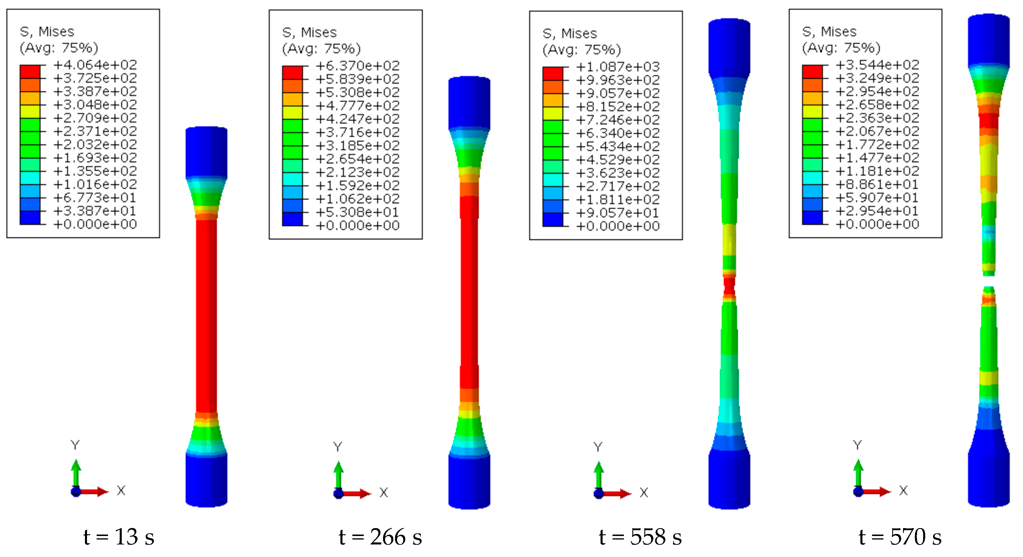
4.2. Finite Element Analysis

The explicit dynamic analysis was executed with a loading time of 684 s. Mass scaling technique was used in the analysis to improve the stability and efficiency of the simulation. This allows for larger time steps and can significantly reduce the computational cost. The scaling factor was set to 2 × 10⁴.

Figure 12 illustrates the variation curves of the internal energy and the kinetic energy throughout the tensile process. The maximum kinetic energy is 343 J, much less than 5% of the internal energy. Therefore, it is reasonable to set the scaling factor to 2 × 10⁴.

The equivalent stress contours at different stages are shown in Figure 13. At the beginning of tensile process, the equivalent stress at gauge section distributes uniformly and is relatively low. As time passes, the specimen gradually elongates while contracting in circumferential direction. The equivalent stress in the gauge range is no longer uniformly distributed and decreases from the center to both ends. When the time reaches 558 s, the center of the specimen is significantly necked with stress concentration. Subsequently, fracture occurs at 570 s.

The strain was calculated based on the relative change in displacement between the two points in Figure 11, before and after tensile loading, with respect to the original gauge length. Subsequently, the load-displacement curve obtained from the simulations was plotted and compared with the corresponding experimental results, demonstrating excellent agreement (Figure 14). Significant fluctuations were observed in the simulation results, shown at the end of the curve. This was due to the occurrence of specimen fracture at this point, and the fracture pattern showed distinct necking, consistent with the experimental results, thus confirming the accuracy of the J-C model parameters.

4.3. Discussions

The validated Johnson–Cook constitutive and damage models’ parameters can be directly applied to the simulation of marine pipeline damage under impact loads. By collecting existing experimental data or conducting tensile tests on different pipe materials, a Johnson–Cook model parameter database can be established. When defining material properties, opting for the Johnson–Cook plasticity and damage model facilitates automatic determination of deformation and fracture occurrences within the model. This choice contributes to a more authentic representation of the pipeline damage process. The identification of the critical damage threshold serves as the basis for establishing the ultimate load capacity of the pipeline. Expanding on this foundational knowledge, an exploration of the interaction between the pipeline, seabed, and water flow forms the groundwork for conducting parameter analyses. These analyses are instrumental in the development of a holistic dynamic damage assessment methodology for marine pipelines.

5. Conclusions

In this paper, quasi-static tensile tests on both smooth round bar and notched round bar and dynamic Hopkinson tensile rod tests were conducted for Q235 steel, which is a commonly used material in marine pipelines. The study successfully determined the eight parameters associated with the J-C constitutive model and failure model, characterizing the mechanical behavior of Q235 steel. The numerical simulations of Q235 steel tensile tests yielded results that corroborated the accuracy of the proposed eight parameters for the J-C constitutive model and failure model. The close agreement between the load–strain curves of the simulations and experimental results, coupled with the observation of distinct necking patterns during fracture, serves as strong evidence supporting the accuracy of the J-C model parameters. The study findings significantly enhance our comprehension of Q235 steel’s mechanical response and failure behavior, especially in diverse loading scenarios, including dynamic events. The insights provide essential inputs for the design and assessment of marine pipelines and other engineering structures, ensuring their reliability and safety in dynamic environments.

References

1. Gao, Q.; Duan, M.; Liu, X.; Wang, Y.; Jia, X.; An, C.; Zhang, T. Damage assessment for submarine photoelectric composite cable under anchor impact. Appl. Ocean. Res. 2018, 73, 42–58. [Google Scholar] [CrossRef]
2. Longva, V.; Sævik, S.; Levold, E.; Ilstad, H. Dynamic simulation of subsea pipeline and trawl board pull-over interaction. Mar. Struct. 2013, 34, 156–184. [Google Scholar] [CrossRef]
3. Ren, J.; Wang, C.; Zahng, X.; Suo, T.; Li, Y.; Tang, Z. Johnson-Cook constitutive model and failure parameters determination of B280VK high-strength steel. J. Plast. Eng. 2023, 30, 116–125. [Google Scholar]
4. Vannucchi de Camargo, F. Survey on Experimental and Numerical Approaches to Model Underwater Explosions. J. Mar. Sci. Eng. 2019, 7, 15. [Google Scholar] [CrossRef]
5. Ellinas, C.P. Ultimate strength of damaged tubular bracing members. J. Struct. Eng. 1984, 110, 245–259. [Google Scholar] [CrossRef]
6. Wierzbicki, T.; Suh, M.S. Indentation of tubes under combined loading. Int. J. Mech. Sci. 1988, 30, 229–248. [Google Scholar] [CrossRef]
7. Bai, Y.; Pedersen, P.T. Elastic-plastic behaviour of offshore steel structures under impact loads. Int. J. Impact Eng. 1993, 13, 99–115. [Google Scholar] [CrossRef]
8. Wang, H.M. Action of Ship Anchoring on Submarine Pipeline in Bohai Bay. Navig. China 2015, 38, 56–59+68. [Google Scholar]
9. DNVGL-ST-F101; Submarine Pipeline Systems. DNV: Bærum, Norway, 2021.
10. DNVGL-RP-F107; Risk Assessment of Pipeline Protection. DNV: Bærum, Norway, 2017.
11. Chen, K.; Shen, W.Q. Further experimental study on the failure of fully clamped steel pipes. Int. J. Impact Eng. 1998, 21, 177–202. [Google Scholar] [CrossRef]
12. Palmer, A.; Neilson, A.; Sivadasan, S. Impact resistance of pipelines and the loss-of-containment limit state. In Proceedings of the International Pipeline Pigging Integrity Assessment and Repair Conference, Calgary, AB, Canada, 4–8 October 2004. [Google Scholar]
13. Palmer, A.; Touhey, M.; Holder, S.; Anderson, M.; Booth, S. Full-scale impact tests on pipelines. Int. J. Impact Eng. 2006, 32, 1267–1283. [Google Scholar] [CrossRef]
14. Zhang, R. Dynamic Response and Failure Mechanism of Structural Tubular Steel Members Subjected to Transverse Impact. Ph.D. Thesis, Harbin Institute of Technology, Shenzhen, China, 2018. [Google Scholar]
15. Zeinoddini, M.; Harding, J.E.; Parke, G.A.R. Effect of impact damage on the capacity of tubular steel members of offshore structures. Mar. Struct. 1998, 11, 141–157. [Google Scholar] [CrossRef]
16. Yan, S.W.; Tian, Y.H. Analysis of pipeline damage to impact load by dropped objects. Trans. Tianjin Univ. 2006, 12, 138–141. [Google Scholar]
17. Huang, Q.F.; Guo, H.Y.; Li, W. Numerical simulation and experimental study on the damage of submarine pipeline impacted by dropped objects. Ocean. Eng. 2018, 36, 84–88. [Google Scholar]
18. Zhang, D.N. A modified Johnson-Cook model of dynamic tensile behaviors for 7075-T6 aluminum alloy. J. Alloys Compd. 2015, 619, 186–194. [Google Scholar] [CrossRef]
19. Banerjee, A.; Dhar, S.; Acharyya, S.; Datta, D.; Nayak, N. Determination of Johnson cook material and failure model constants and numerical modelling of Charpy impact test of armour steel. Mater. Sci. Eng. A 2015, 640, 200–209. [Google Scholar] [CrossRef]
20. Cao, Y.; Zhen, Y.; Song, M.; Yi, H.; Li, F.; Li, X. Determination of Johnson–Cook parameters and evaluation of Charpy impact test performance for X80 pipeline steel. Int. J. Mech. Sci. 2020, 179, 105627. [Google Scholar] [CrossRef]
21. Wang, Z.; Hu, Z.; Liu, K.; Chen, G. Application of a material model based on the Johnson-Cook and Gurson-Tvergaard-Needleman model in ship collision and grounding simulations. Ocean. Eng. 2020, 205, 106768. [Google Scholar] [CrossRef]
22. Wang, X.M.; Shi, J. Validation of Johnson-Cook plasticity and damage model using impact experiment. Int. J. Impact Eng. 2023, 60, 67–75. [Google Scholar] [CrossRef]
23. Aktürk, M.; Boy, M.; Gupta, M.K.; Waqar, S.; Krolczyk, G.M.; Korkmaz, M.E. Numerical and experimental investigations of built orientation dependent Johnson-Cook model for selective laser melting manufactured AlSi10Mg. J. Mater. Res. Technol. 2021, 15, 6244–6259. [Google Scholar] [CrossRef]
24. Deshpande, V.M.; Chakraborty, P.; Chakraborty, T.; Tiwari, V. Application of copper as a pulse shaper in SHPB tests on brittle materials-experimental study, constitutive parameters identification, and numerical simulations. Mech. Mater. 2022, 171, 104336. [Google Scholar] [CrossRef]
25. Daoud, M.; Chatelain, J.F.; Bouzid, A. Effect of rake angle-based Johnson-Cook material constants on the prediction of residual stresses and temperatures induced in Al2024-T3 machining. Int. J. Mech. Sci. 2017, 122, 392–404. [Google Scholar] [CrossRef]
26. Chao, Z.L.; Jiang, L.T.; Chen, G.Q.; Zhang, Q.; Zhang, N.B.; Zhao, Q.Q.; Pang, B.J.; Wu, G.H. A modified Johnson-Cook model with damage degradation for B4Cp/Al composites. Compos. Struct. 2022, 282, 115029. [Google Scholar] [CrossRef]
27. Liu, Y.; Li, M.; Ren, X.W.; Xiao, Z.B.; Zhang, X.Y.; Huang, Y.C. Flow stress prediction of Hastelloy C-276 alloy using modified Zerilli-Armstrong, Johnson-Cook and Arrhenius-type constitutive models. Trans. Nonferrous Met. Soc. China 2020, 30, 3031–3042. [Google Scholar] [CrossRef]
28. Xie, G.; Yu, X.; Gao, Z.; Xue, W.; Zheng, L. The modified Johnson-Cook strain-stress constitutive model according to the deformation behaviors of a Ni-W-Co-C alloy. J. Mater. Res. Technol. 2022, 20, 1020–1027. [Google Scholar] [CrossRef]
29. Wei, G.; Zhang, W.; Deng, Y.F. Identification and validation of constitutive parameters of 45 Steel based on J-C model. J. Vib. Shock. 2019, 38, 173–178. [Google Scholar]
30. Zhu, Y. Research on Dynamic Constitutive Relationship of Q355B Steel Based on Johnson-Cook Model. Ph.D. Thesis, Harbin University of Science and Technology, Harbin, China, 2019. [Google Scholar]
31. Chen, J.L.; Shu, W.Y.; Li, J.W. Experimental study on dynamic mechanical property of Q235 steel at different strain rates. J. Tongji Univ. 2016, 44, 1071–1075. [Google Scholar]
32. Chen, X.W.; Wei, L.M.; Li, J.C. Experimental research on the long rod penetration of tungsten-fiber/Zr-based metallic glass matrix composite into Q235 steel target. Int. J. Impact Eng. 2015, 79, 102–116. [Google Scholar] [CrossRef]
33. Guo, Z.T.; Gao, B.; Guo, Z.; Zhang, W. Dynamic constitutive relation based on J-C model of Q235 steel. Explos. Shock. Waves 2018, 38, 804–810. [Google Scholar]
34. Shokry, A.; Gowid, S.; Mulki, H.; Kharmanda, G. On the Prediction of the Flow Behavior of Metals and Alloys at a Wide Range of Temperatures and Strain Rates Using Johnson–Cook and Modified Johnson–Cook-Based Models: A Review. Materials 2023, 16, 1574. [Google Scholar] [CrossRef]
35. Sirigiri VK, R.; Gudiga, V.Y.; Gattu, U.S.; Suneesh, G.; Buddaraju, K.M. A review on Johnson Cook material model. Mater. Today Proc. 2022, 62, 3450–3456. [Google Scholar] [CrossRef]
36. Carra, F.; Charrondiere, C.; Guinchard, M.; Sacristan de Frutos, O. Design and construction of an instrumentation system to capture the response of advanced materials impacted by intense proton pulses. Shock. Vib. 2021, 2021, 8855582. [Google Scholar] [CrossRef]
Figure 1. The dimensions of smooth tensile specimens (Unit: mm).
Jmse 11 01666 g001
Figure 2. Stress–strain curves of smooth round bar quasi-static tensile tests.
Jmse 11 01666 g002
Figure 3. ln σ A - ln ε fitted curves.
Jmse 11 01666 g003
Figure 4. The dimensions of the notched specimen (Unit: mm).
Jmse 11 01666 g004
Figure 5. Stress–strain curve of specimens with different notches.
Jmse 11 01666 g005
Figure 6. Failure strain versus stress-state curve.
Jmse 11 01666 g006
Figure 7. Test principle of split Hopkinson tensile bar device.
Jmse 11 01666 g007
Figure 8. The dimensions of the Hopkinson tensile specimens (Unit: mm).
Jmse 11 01666 g008
Figure 9. The fitted curve of equivalent stress vs. dimensionless strain rate.
Jmse 11 01666 g009
Figure 10. The fitted curve of failure strain vs. dimensionless strain rate.
Jmse 11 01666 g010
Figure 11. The meshed model.
Jmse 11 01666 g011
Figure 12. Curves of internal energy and kinetic energy.
Jmse 11 01666 g012
Figure 13. Contours of equivalent stress at different stages.
Jmse 11 01666 g013
Figure 14. Comparison of load–strain curves between experimental and numerical results.
Jmse 11 01666 g014