Particle Filter Based on Harris Hawks Optimization Algorithm for Underwater Visual Tracking

Abstract

Due to the complexity of the underwater environment, tracking underwater targets via traditional particle filters is a challenging task. To resolve the problem that the tracking accuracy of a traditional particle filter is low due to the sample impoverishment caused by resampling, in this paper, a new tracking algorithm using Harris-hawks-optimized particle filters (HHOPF) is proposed. At the same time, the problem of particle filter underwater target feature construction and underwater target scale transformation is addressed, the corrected background-weighted histogram method is introduced into underwater target feature recognition, and the scale filter is combined to realize target scaling transformation during tracking. In addition, to enhance the computational speed of underwater target tracking, this paper constructs a nonlinear escape energy using the Harris hawks algorithm in order to balance the exploration and exploitation processes. Based on the proposed HHOPF tracker, we performed detection and evaluation using the Underwater Object Tracking (UOT100) vision database. The proposed method is compared with evolution-based tracking algorithms and particle filters, as well as with recent tracker-based correlation filters and some other state-of-the-art tracking methods. By comparing the results of tracking using the test data sets, it is determined that the presented algorithm improves the overlap accuracy and tracking accuracy by 11% compared with other algorithms. The experiments demonstrate that the presented HHOPF visual tracking provides better tracking results.

1. Introduction

With the progress in research on computer vision, visual tracking has become a key research problem. At present, visual tracking has been used in various applications, such as vision-based robotics [1], surveillance systems [2], and ship tracking [3]. The above shows that a significant amount of work has been carried out on visual tracking, but most of it has been conducted on land-based targets; although most of the world is covered by the ocean, less work has been performed on underwater monitoring. Therefore, the present demand is gradually focusing on the design and development of underwater monitoring systems, and the main research considerations of underwater monitoring systems are target detection [4,5] and tracking [6].

Due to the quality of the marine environment and the hardware problems of the main equipment, it is easy to produce fog, occlusion, poor contrast, and improper lighting [7], which makes the tracking of underwater scenes extremely challenging. Because of these problems, in addition to improving the equipment hardware, numerous scholars have made a variety of improvements to the tracking method to adapt it to additional application scenarios.

In recent years, visual target tracking based on correlation filters (CF) and Siamese networks has made significant progress. Wang et al. [8] improved the kernel correlation filter (KCF) by using a dynamic continuous change scale and adaptive filter update strategy which can better predict the position of an underwater target; better tracking effects can be achieved with this improvement. Faced with the complexity of the underwater environment, Wu et al. [9] presented an improved Siamese network which introduced a lightweight network and hybrid excitation model to reduce the computational complexity and enhance the network’s accuracy to achieve better underwater target tracking. Hong et al. [10] proposed an improved YOLOv4 algorithm that simplifies the feature extraction layer network and uses a residual network instead of continuous convolution operation, thereby improving the poor real-time operation and low accuracy of multi-ship target tracking.

Although many deep-learning methods are now applied to underwater environments, due to the characteristics of deep-learning training, it is currently difficult to track targets in real-time using underwater equipment. Currently, generative tracking methods such as particle filters are still the ideal choice for tracking methods used in underwater equipment. Particle filter (PF) algorithms have become some of the most widely used algorithms because of their advantages in the face of nonlinear problems, but particle filters also have some problems with respect to visual tracking. Therefore, the improvement in particle filter tracking algorithms plays an important role in improving the application of underwater equipment.

Currently, the use of a particle filter in tracking is influenced by three main themes: a consistent observation model, a precise motion model, and sample impoverishment. These thematic influences are generally considered the main idea for investigating particle filtering results. To solve these problems, this paper presented a particle filter method based on Harris hawks optimization (HHO). This filter contains the exploration and exploitation process of an optimization algorithm for a sample impoverishment problem in order to resolve the inherent problems of the particle filter and improve target tracking results. The main contributions of this work are:

• To resolve the problem of sample impoverishment caused by continuous resampling during the tracking process of the particle filter. The HHOPF algorithm is proposed to guide the swarm of particles to move to the region of high-likelihood probability density before the resampling process in order to ensure the diversity of samples.
• To enhance the capability of the algorithm in underwater target feature extraction, this paper introduces a corrected background-weighted histogram to improve the target feature extraction. Meanwhile, we propose a method combining a scale filter and particle filter to solve the target scale transformation, which improves the target tracking method’s performance.
• To improve the tracking performance, a new nonlinear escape energy is constructed for use in the Harris hawks algorithm so that it can balance the exploration and exploitation processes, better carry out global exploration and local development, and improve tracking results.
• The performance of the proposed HHOPF algorithm is qualitatively and quantitatively analyzed in comparison with other tracking algorithms, including particle filters based on evolutionary optimization, recent correlation filters, and other advanced tracking algorithms.

The rest of the paper is introduced as follows, and the details will be expanded upon in the corresponding sections. Section 2 introduces the related works regarding particle filter improvement. Section 3 introduces the particle filter (PF) and Harris hawks optimization algorithm (HHO). Section 4 explains the presented Harris-hawks-optimized particle filter (HHOPF). In Section 5, the presented tracker is analyzed in combination with other advanced tracking methods, and the tracking experimental results are discussed. Section 6 provides a summary of the paper and a future work plan.

2. Related Work

Given the existing problems of the particle filter, its improvement strategies mainly include improvement based on the observation model, improvement based on the motion model, and improvement based on sample impoverishment.

2.1. Improved Particle Filter Based on the Observation Model

In visual target tracking, the observation model of the particle filter is the expression of the characteristic information of the tracking target. If the observation model is well constructed, the characteristic information of the tracking target is closer to that of the real target, so that better tracking can be obtained. Therefore, to build a more robust observation model, researchers have changed from the initial color histogram representation of the target information to the current multi-feature [11] fusion in order to construct an observation model to represent the feature information of the target. For example, Dai et al. [12] proposed a multi-feature fusion method combining a color feature and an LBP texture feature to address the object occlusion and deformation in some simple scenes. The observation model of the particle filter constructed using the multi-feature fusion method can enhance the tracking performance but also increase the computational complexity.

2.2. Improved Particle Filter Based on the Motion Model

The motion model of the particle filter affects the tracking performance by influencing the prediction of the target position. The different motion characteristics of the tracking target can be described as translation, rotation, and the change in object size. At present, the particle filter adopts a constant velocity motion model for the translation motion and a random walk model for the rotation and scaling. In addition, Brasnett et al. [13] proposed a multi-component state motion model to track the target by combining the constant velocity motion model and the random walk model in a particle filter. However, due to the complexity of the practical application scenarios, it is still difficult to have a unified motion model that satisfies all environmental conditions.

2.3. Improved Particle Filter Based on Sample Impoverishment

In the particle filter, the weighted sum of the sample particles of the simulated target reflects the real state of the target, and the sampling quality of the sample particles directly affects the tracking result. Given sample impoverishment in the particle filter, some researchers reduce sample impoverishment by improving the resampling process, such as in adaptive resampling [14], systematic resampling, and residual resampling. Due to the fact that the particles cannot be restored, most of these methods solve the problem only to a certain extent. Other researchers solve the sample impoverishment by approximating probability density functions (PDF). In this category, researchers proposed an unscented particle filter and an extended Kalman particle filter [15]. However, under the probability density function proposed in the above method, the obtained results do not satisfy the requirements and introduce additional computational power.

In recent years, with the application of different evolutionary optimization algorithms in various scenarios [16,17,18], some researchers have studied them in combination with visual tracking problems and made significant progress. By combining an evolutionary optimization algorithm with the particle filter, the researchers [19,20] found that the evolutionary algorithm does not depend on the prior knowledge of the particle filter, and can be explored and exploited in the face of uncertainty so that the particles show arbitrariness. Based on this characteristic, it can improve the particle impoverishment problem by combining the particle filter with an evolutionary optimization algorithm. However, the above work is tested in the case of a nonlinear function, without further verification of the video sequences, so there are shortcomings. To resolve the problem of sample impoverishment of the particle filter in target tracking, an optimized auxiliary particle filter algorithm based on spider monkey was proposed in the literature [21]. Nenavath et al. [22] presented guidance regarding particle position by using a sine cosine optimization algorithm. Currently, there are still some problems with respect to the work: (1) The swarm optimization algorithm has a poor convergence ability and little optimization of parameters. (2) In the face of the target transformation, the particle filter takes a long time to estimate the scale of all particles. (3) The particle filter does not consider the background information, so errors are easily caused in the tracking.

3. Particle Filter and Harris Hawks Optimization Algorithm

The proposed HHOPF mainly consists of two parts: one is the tracking framework of the improved particle filter, and the other is the improved Harris hawks optimization algorithm. Next, we introduce the principle of the initial state of these two major parts and explain their application in the proposed algorithm.

3.1. Particle Filter

A particle filter is a recursive Bayesian filter algorithm based on the Monte Carlo method. The particle filter can be used in any state-space description of a system, the core of which is to construct a posteriori probability density function that reflects the real particle distribution. A particle filter mainly has two steps:

• Prediction: Use a motion model to predict the state.
• Update: Use an observation model to update the status.

Recursively apply these steps to obtain the probability density function $\mathrm{p}\left({\mathrm{x}}_{\mathrm{k}}|{\mathrm{y}}_{1:\mathrm{k}}\right)$.

In a particle filter, a posteriori probability density $\mathrm{p}\left({\mathrm{x}}_{\mathrm{k}}|{\mathrm{y}}_{1:\mathrm{k}}\right)$ is approximately a finite set of N samples (particles) ${\{{\mathrm{x}}_{\mathrm{k}}^{\mathrm{i}},{\mathrm{w}}_{\mathrm{k}}^{\mathrm{i}}\}}_{\mathrm{i}=0}^{\mathrm{N}}$, where ${\mathrm{w}}_{\mathrm{k}}^{\mathrm{i}}$ is the importance weight:

$$\mathrm{p}\left({\mathrm{x}}_{\mathrm{k}}|{\mathrm{y}}_{1:\mathrm{k}}\right)=\sum _{\mathrm{i}=1}^{\mathrm{N}}{\mathrm{w}}_{\mathrm{k}}^{\mathrm{i}}\mathsf{\delta }\left({\mathrm{x}}_{\mathrm{k}}-{\mathrm{x}}_{\mathrm{k}}^{\mathrm{i}}\right)$$

(1)

where ${\mathrm{y}}_{1:\mathrm{k}}$ is the set of the observed values accumulated with time k, that is ${\mathrm{y}}_{1:\mathrm{k}}=\{{\mathrm{y}}_1,{\mathrm{y}}_2,\dots ,{\mathrm{y}}_{\mathrm{k}}\}$.

However, in the actual process of using the particle filter, it is often not possible to sample straightway from the PDF of the target state, because the PDF $\mathrm{p}\left({\mathrm{x}}_{\mathrm{k}}|{\mathrm{y}}_{1:\mathrm{k}}\right)$ will be multi-variable or other distribution cases that are not standard. Thus, the proposed density function $\mathrm{q}\left({\mathrm{x}}_{\mathrm{k}}^{\mathrm{i}}|{\mathrm{x}}_{\mathrm{k}-1}^{\mathrm{i}},{\mathrm{y}}_{\mathrm{k}}\right)$ is proposed, and the particles are sampled. To better describe the target state, the probability distribution of the proposed density function is frequently set to be the same as $\mathrm{p}\left({\mathrm{x}}_{\mathrm{k}}|{\mathrm{y}}_{1:\mathrm{k}}\right)$. In importance weight, the weight is updated by Formula (2):

$${\mathrm{w}}_{\mathrm{k}}^{\mathrm{i}}\propto {\mathrm{w}}_{\mathrm{k}-1}^{\mathrm{i}}\frac{\mathrm{p}\left({\mathrm{y}}_{\mathrm{k}}|{\mathrm{x}}_{\mathrm{k}}^{\mathrm{i}}\right)\mathrm{p}\left({\mathrm{x}}_{\mathrm{k}}^{\mathrm{i}}|{\mathrm{x}}_{\mathrm{k}-1}^{\mathrm{i}}\right)}{\mathrm{q}\left({\mathrm{x}}_{\mathrm{k}}^{\mathrm{i}}|{\mathrm{x}}_{\mathrm{k}-1}^{\mathrm{i}},{\mathrm{y}}_{\mathrm{k}}\right)}$$

(2)

In a particle filter with the tracking process, except for a few particles the weight of other particles gradually becomes negligible. Therefore, substantial computation is wasted on updating the invalid particles (small-weight particles), which can gravely affect the performance of the particle filter. To resolve this problem, the resampling process is introduced. The resampling process consists of sampling the particle set ${\left\{{\mathrm{x}}_{\mathrm{k}}^{\mathrm{i}}|{\mathrm{w}}_{\mathrm{k}}^{\mathrm{i}}\right\}}_{\mathrm{i}=1}^{\mathrm{N}}$ again, according to the weights of the particles. During the sampling process, the particles with a larger weight are repeatedly extracted, while those with a smaller weight are eliminated.

Although the resampling process can eliminate the effect of the smaller weighted particles, the resampling procedure can also introduce a new negative problem, namely sample impoverishment. This is because throughout the multiple resampling processes, the excessive replication of the high-weight particles reduces the number of meaningful particles, resulting in a serious reduction in the effective information in the new particle set. In a particle filter, the effective particle number is defined as follows:

$$\mathrm{N}\mathrm{e}\mathrm{f}\mathrm{f}=\frac{1}{{\sum }_{\mathrm{i}=1}^{\mathrm{N}}{\left({\mathrm{w}}_{\mathrm{k}}^{\mathrm{i}}\right)}^2}$$

(3)

In target tracking, we describe the target state by the particle state. The number of effective particles of the PF is severely reduced after repeated recursive calculations in the process of prediction and updating, so it is difficult for the particle set obtained after resampling to reflect the target state. Therefore, to resolve this problem, the HHO algorithm is combined to achieve better target state estimation by guiding the particle motion.

3.2. Harris Hawks Optimization Algorithm

Harris hawks optimization algorithm is an intelligent swarm optimization algorithm proposed by Heidari et al. [23]. It mimics the behavior of a rabbit-hunting hawk, which responds to the different states of the rabbit and its escape strategies to ensure its hunt. The process of the principle includes the location update in the exploration process and four convergence strategies in the exploitation process.

Its behavior is as follows:

$$\mathrm{E}=2{\mathrm{E}}_0\left(1-\frac{\mathrm{t}}{\mathrm{T}}\right)$$

(4)

where $\mathrm{E}$ represents the the prey’s energy, $\mathrm{T}$ is the maximum iterations, and ${\mathrm{E}}_0$ is the initial state’s energy.

If $\left|\mathrm{E}\right|\ge 1$ enters the exploration phase, then search for the target; if $\left|\mathrm{E}\right|<1$ enters the exploitation phase, then approach the target for capture.

(1)

Exploration phase ($\left|\mathrm{E}\right|\ge 1$):

$$\mathrm{X}\left(\mathrm{t}+1\right)=\left\{\begin{array}{ll}{\mathrm{X}}_{\mathrm{r}\mathrm{a}\mathrm{n}\mathrm{d}}\left(\mathrm{t}\right)-{\mathrm{r}}_1\left|{\mathrm{X}}_{\mathrm{r}\mathrm{a}\mathrm{n}\mathrm{d}}\left(\mathrm{t}\right)-2{\mathrm{r}}_2\mathrm{X}\left(\mathrm{t}\right)\right|& \mathrm{q}\ge 0.5\\ \left({\mathrm{X}}_{\mathrm{r}\mathrm{a}\mathrm{b}\mathrm{b}\mathrm{i}\mathrm{t}}\left(\mathrm{t}\right)-{\mathrm{X}}_{\mathrm{m}}\left(\mathrm{t}\right)\right)-{\mathrm{r}}_3\left(\mathrm{L}\mathrm{B}+{\mathrm{r}}_4\left(\mathrm{U}\mathrm{B}-\mathrm{L}\mathrm{B}\right)\right)& \mathrm{q}\le 0.5\end{array}\right.$$

(5)

where $\mathrm{X}\left(\mathrm{t}\right)$ is the position vector of the hawk in the current iteration, ${\mathrm{X}}_{\mathrm{r}\mathrm{a}\mathrm{b}\mathrm{b}\mathrm{i}\mathrm{t}}\left(\mathrm{t}\right)$ is the position vector of the rabbit, ${\mathrm{r}}_1,{\mathrm{r}}_2,{\mathrm{r}}_3,{\mathrm{r}}_4$, and $\mathrm{q}$ are updated in each iteration and their values are random numbers in (0, 1), $\mathrm{L}\mathrm{B}$ and $\mathrm{U}\mathrm{B}$, respectively, represent the upper and lower boundaries of variable coordinates in the iteration process of the algorithm, ${\mathrm{X}}_{\mathrm{r}\mathrm{a}\mathrm{n}\mathrm{d}}\left(\mathrm{t}\right)$ is a random individual selected from the hawks, and ${\mathrm{X}}_{\mathrm{m}}$ is the mean of the positions of all hawks.

(2)

Exploitation phase ($\left|\mathrm{E}\right|<1$):

Let r be the probability that the rabbit successfully escapes (r < 0.5) or the probability that the rabbit does not (r > 0.5).

(1)

Soft besiege $\left(\mathrm{r}\ge 0.5 \mathrm{a}\mathrm{n}\mathrm{d} \left|\mathrm{E}\right|\ge 0.5\right)$:

$$\mathrm{X}\left(\mathrm{t}+1\right)=∆\mathrm{X}\left(\mathrm{t}\right)-\mathrm{E}\left|\mathrm{J}{\mathrm{X}}_{\mathrm{r}\mathrm{a}\mathrm{b}\mathrm{b}\mathrm{i}\mathrm{t}}\left(\mathrm{t}\right)-\mathrm{X}\left(\mathrm{t}\right)\right|$$

(6)

$$∆\mathrm{X}\left(\mathrm{t}\right)={\mathrm{X}}_{\mathrm{r}\mathrm{a}\mathrm{b}\mathrm{b}\mathrm{i}\mathrm{t}}\left(\mathrm{t}\right)-\mathrm{X}\left(\mathrm{t}\right)$$

(7)

where $∆\mathrm{X}\left(\mathrm{t}\right)$ is the difference between the position vector of the prey in the current iteration and iteration t, ${\mathrm{r}}_5$ is the random digit in (0,1), and $\mathrm{J}=2(1-{\mathrm{r}}_5)$ expresses the random jump intensity J.

(2)

Hard besiege $(\mathrm{r}\ge 0.5 \mathrm{a}\mathrm{n}\mathrm{d} \left|\mathrm{E}\right|<0.5)$:

$$\mathrm{X}\left(\mathrm{t}+1\right)={\mathrm{X}}_{\mathrm{r}\mathrm{a}\mathrm{b}\mathrm{b}\mathrm{i}\mathrm{t}}\left(\mathrm{t}\right)-\mathrm{E}\left|∆\mathrm{X}\left(\mathrm{t}\right)\right|$$

(8)

(3)

Soft besiege with progressive rapid dives $\left(\mathrm{r}<0.5 \mathrm{a}\mathrm{n}\mathrm{d} \left|\mathrm{E}\right|\ge 0.5\right)$:

$$\mathrm{X}\left(\mathrm{t}+1\right)=\left\{\begin{array}{cc}\mathrm{Y}& \mathrm{if}\mathrm{F}\left(\mathrm{Y}\right)<\mathrm{F}\left(\mathrm{X}\left(\mathrm{t}\right)\right)\\ \mathrm{Z}& \mathrm{if}\mathrm{F}\left(\mathrm{Z}\right)<\mathrm{F}\left(\mathrm{X}\left(\mathrm{t}\right)\right)\end{array}\right.$$

(9)

$$\mathrm{Y}={\mathrm{X}}_{\mathrm{r}\mathrm{a}\mathrm{b}\mathrm{b}\mathrm{i}\mathrm{t}}\left(\mathrm{t}\right)-\mathrm{E}\left|\mathrm{J}{\mathrm{X}}_{\mathrm{r}\mathrm{a}\mathrm{b}\mathrm{b}\mathrm{i}\mathrm{t}}\left(\mathrm{t}\right)-\mathrm{X}\left(\mathrm{t}\right)\right|$$

(10)

$$\mathrm{Z}=\mathrm{Y}+\mathrm{S}\times \mathrm{L}\mathrm{F}\left(\mathrm{D}\right)$$

(11)

$$\mathrm{L}\mathrm{F}\left(\mathrm{x}\right)=0.01\times \frac{\mathrm{u}\times \mathsf{\sigma }}{{\left|\mathrm{v}\right|}^{\frac{1}{\mathsf{\beta }}}},\mathsf{\sigma }={\left(\frac{\mathsf{\Gamma }\left(1+\mathsf{\beta }\right)\times \sin \frac{\mathsf{\pi }\mathsf{\beta }}{2}}{\mathsf{\Gamma }\left(\frac{1+\mathsf{\beta }}{2}\right)\times \mathsf{\beta }\times 2^{\left(\frac{\mathsf{\beta }-1}{2}\right)}}\right)}^{\frac{1}{\mathsf{\beta }}}$$

(12)

where $\mathrm{D}$ is the dimension, $\mathrm{S}$ is a random vector of size $1\times \mathrm{D}$, and ${\mathrm{L}}_{\mathrm{f}}$ is the levy flight function. $\mathrm{u},\mathsf{\upsilon }$ is a random value within (0, 1) and β is the default constant set at 1.5.

(4)

Hard besiege with progressive rapid dives $(\mathrm{r}<0.5 \mathrm{a}\mathrm{n}\mathrm{d} \left|\mathrm{E}\right|<0.5)$:

$$\mathrm{X}\left(\mathrm{t}+1\right)=\left\{\begin{array}{cc}\mathrm{Y}& \mathrm{if}\mathrm{F}\left(\mathrm{Y}\right)<\mathrm{F}\left(\mathrm{X}\left(\mathrm{t}\right)\right)\\ \mathrm{Z}& \mathrm{if}\mathrm{F}\left(\mathrm{Z}\right)<\mathrm{F}\left(\mathrm{X}\left(\mathrm{t}\right)\right)\end{array}\right.$$

(13)

$$\mathrm{Y}={\mathrm{X}}_{\mathrm{r}\mathrm{a}\mathrm{b}\mathrm{b}\mathrm{i}\mathrm{t}}\left(\mathrm{t}\right)-\mathrm{E}\left|\mathrm{J}{\mathrm{X}}_{\mathrm{r}\mathrm{a}\mathrm{b}\mathrm{b}\mathrm{i}\mathrm{t}}\left(\mathrm{t}\right)-{\mathrm{X}}_{\mathrm{m}}\left(\mathrm{t}\right)\right|$$

(14)

$$\mathrm{Z}=\mathrm{Y}+\mathrm{S}\times \mathrm{L}\mathrm{F}\left(\mathrm{D}\right)$$

(15)

where ${\mathrm{X}}_{\mathrm{m}}\left(\mathrm{t}\right)$ is obtained using the formula ${\mathrm{X}}_{\mathrm{m}}\left(\mathrm{t}\right)=\frac{1}{\mathrm{N}}{\sum }_{\mathrm{i}=1}^{\mathrm{N}}{\mathrm{X}}_{\mathrm{i}}\left(\mathrm{t}\right)$.

In the proposed algorithm, if the number of effective particles in the PF is reduced, the particles will fail to reflect the real target state. To address this problem, we will enter the iterative optimization process of the optimization algorithm. In this process, we treat the prey and predators as particles, simulating the process of exploration and exploitation. In this way, the position of the particles can be optimized to improve the target state expression. The details of the HHOPF algorithm are explained in the following.

4. Visual Tracking Based on Harris Hawks Optimized Particle Filter

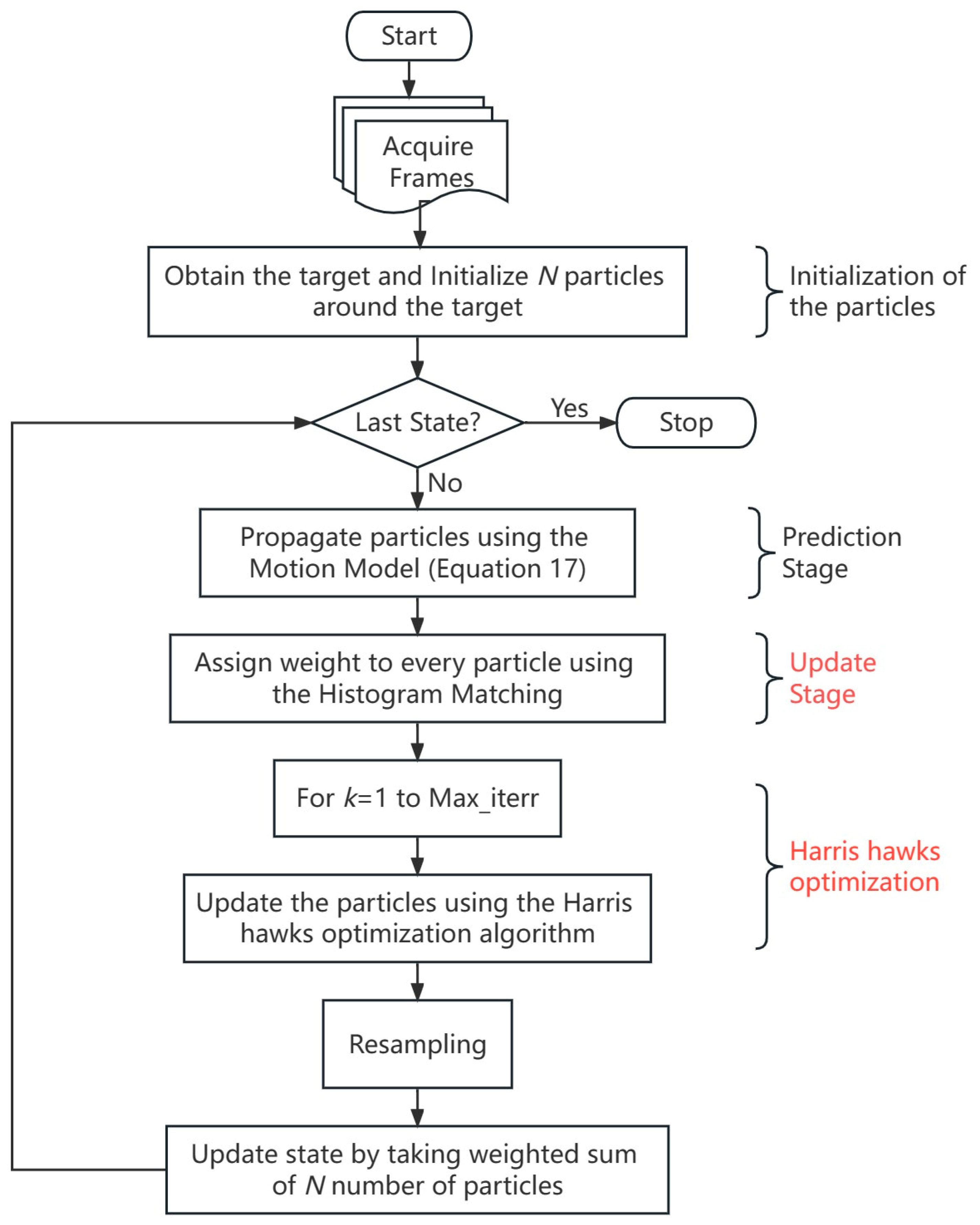
In this section, we describe a detailed explanation of our presented HHOPF algorithm. In the update status and Harris hawks optimization part, the principle of the proposed innovation points is expounded. The simplified schematic diagram is shown in Figure 1.

Figure 1. The simplified schematic diagram of the HHOPF.

4.1. Motion Model

With the continuous development of the tracking methods, researchers have also made continuous improvements to the motion models. Now, common motion models include constant velocity (CV), constant acceleration (CA), random walk (RW), and multi-component state models. In our experiments, we guide the motion of the target object state via a model of constant velocity motion. The instantaneous state expression for the target object can be obtained using $\left(\mathbf{x},\dot{\mathbf{x}},\mathbf{y},\dot{\mathbf{y}}\right)$, including $\left(\mathbf{x},\mathbf{y}\right)$, and $\left(\dot{\mathbf{x},}\dot{\mathbf{y}}\right)$, which are the 2D center coordinates and velocity of the target object, respectively. Equation (16) expresses the target state:

$$\mathbf{X}=\left(\mathbf{x},\dot{\mathbf{x}},\mathbf{y},\dot{\mathbf{y}}\right)$$

(16)

Equations are used to evaluate the motion state and the likelihood that the motion of the object is expected to spread at any time:

$${\mathbf{X}}_{\mathbf{k}+\mathbf{1}}=\mathbf{E}{\mathbf{X}}_{\mathbf{k}}+{\mathsf{\eta }}_{\mathbf{k}};\hspace{1em}\hspace{1em}{\mathsf{\eta }}_{\mathbf{k}}~\left(0,\mathbf{M}\right)$$

(17)

$$\mathbf{E}=\left[\begin{array}{cc}\left(\begin{array}{cc}1& \mathrm{B}\\ 0& 1\end{array}\right)& 0_{2\times 2}\\ 0_{2\times 2}& \left(\begin{array}{cc}1& \mathrm{B}\\ 0& 1\end{array}\right)\end{array}\right]$$

The covariance matrix in the constant velocity state motion model can be expressed as follows:

$$\mathbf{M}=\left[\begin{array}{cc}{\mathbf{M}}_{\mathbf{x}}& 0_{2\times 2}\\ 0_{2\times 2}& {\mathbf{M}}_{\mathbf{y}}\end{array}\right]$$

${\mathsf{\eta }}_{\mathbf{k}}$ is a Gaussian white noise with zero mean, $\mathrm{B}$ is the interval in which the sample is taken, and $\mathbf{M}$ has determined the covariance of value $({\mathsf{\sigma }}_{\mathrm{x}}^2,{\mathsf{\sigma }}_{\mathrm{y}}^2)$.

4.2. Observation Model

4.2.1. Representation of the Target

In target tracking, it is common to divide the target object into a range of boxes in a frame to express the target and use a color histogram to express the information about the object. The object region is regularized into n pixels and is denoted by ${\left\{{\mathrm{x}}_{\mathrm{i}}^{\mathrm{*}}\right\}}_{\mathrm{i}=1,2,\dots ,\mathrm{n}}$. We can obtain the object model via the following equation:

$$\widehat{\mathrm{q}}={\left\{{\widehat{\mathrm{q}}}_{\mathrm{u}}\right\}}_{\mathrm{u}=1,2,\dots ,\mathrm{m}}$$

(18)

$${\widehat{\mathrm{q}}}_{\mathrm{u}}=\mathrm{C}\sum _{\mathrm{i}=1}^{\mathrm{n}}\mathrm{k}\left(‖{\mathrm{x}}_{\mathrm{i}}^{\mathrm{*}}‖\right)·\mathsf{\delta }\left[\mathrm{b}\left({\mathrm{x}}_{\mathrm{i}}^{\mathrm{*}}\right)-\mathrm{u}\right]$$

(19)

where $\widehat{\mathrm{q}}$ is the object model and ${\widehat{\mathrm{q}}}_{\mathrm{u}}$ is the possibility that the U-th element of $\mathrm{b}\left({\mathrm{x}}_{\mathrm{i}}^{\mathrm{*}}\right)$ belongs to the histogram of pixel ${\mathrm{x}}_{\mathrm{i}}^{\mathrm{*}}$.

4.2.2. Corrected Background-Weighted Histogram

In target tracking, scholars have shown that the ability to accurately locate the target will be affected if the representational information between the object and the background is close. Therefore, considering the treatment of the background information, a corrected background-weighted histogram strategy is introduced, which can improve the accurate localization of the target by constraining the target background elements. After the target histogram is corrected, the target model is shown in Equation:

$${\widehat{\mathrm{q}}}_{\mathrm{u}}={\mathrm{C}}_1{\mathsf{\upsilon }}_{\mathrm{u}}\sum _{\mathrm{i}=1}^{\mathrm{n}}\mathrm{k}\left({‖{\mathrm{x}}_{\mathrm{i}}^{\mathrm{*}}‖}^2\right)·\mathsf{\delta }\left[\mathrm{b}\left({\mathrm{x}}_{\mathrm{i}}^{\mathrm{*}}\right)-\mathrm{u}\right]$$

(20)

The regularization constant is:

$${\mathrm{C}}_1=\frac{1}{{\sum }_{\mathrm{i}=1}^{\mathrm{n}}\mathrm{k}\left({‖{\mathrm{x}}_{\mathrm{i}}^{\mathrm{*}}‖}^2\right){\sum }_{\mathrm{u}=1}^{\mathrm{m}}{\mathsf{\upsilon }}_{\mathrm{u}}\mathsf{\delta }\left[\mathrm{b}\left({\mathrm{x}}_{\mathrm{i}}^{\mathrm{*}}\right)-\mathrm{u}\right]}$$

(21)

The target candidate model expression is:

$${\widehat{\mathrm{p}}}_{\mathrm{u}}={\mathrm{C}}_{\mathrm{h}}{\mathsf{\upsilon }}_{\mathrm{u}}\sum _{\mathrm{i}=1}^{{\mathrm{n}}_{\mathrm{h}}}\mathrm{k}\left({‖\frac{\mathrm{y}-{\mathrm{x}}_{\mathrm{i}}}{\mathrm{h}}‖}^2\right)·\mathsf{\delta }\left[\mathrm{b}\left({\mathrm{x}}_{\mathrm{i}}\right)-\mathrm{u}\right]$$

(22)

$${\mathrm{C}}_{\mathrm{h}}=\sum _{\mathrm{i}=1}^{{\mathrm{n}}_{\mathrm{h}}}\mathrm{k}\left({‖\frac{\mathrm{y}-{\mathrm{x}}_{\mathrm{i}}}{\mathrm{h}}‖}^2\right)\sum _{\mathrm{u}=1}^{\mathrm{m}}{\mathsf{\upsilon }}_{\mathrm{u}}\mathsf{\delta }\left[\mathrm{b}\left({\mathrm{x}}_{\mathrm{i}}\right)-\mathrm{u}\right]$$

(23)

$$\sum _{\mathrm{i}=1}^{\mathrm{m}}{\widehat{\mathrm{O}}}_{\mathrm{u}}=1$$

(24)

$${\mathsf{\upsilon }}_{\mathrm{u}}=\mathrm{m}\mathrm{i}\mathrm{n}\left(\frac{\widehat{\mathrm{O}}}{{\widehat{\mathrm{O}}}_{\mathrm{u}}},1\right)$$

(25)

where $\widehat{\mathrm{O}}$ is the background statistics ${\left\{{\widehat{\mathrm{O}}}_{\mathrm{u}}\right\}}_{\mathrm{u}=1,2,\dots ,\mathrm{m}}$ of the non-zero minimum value.

In the corrected condition, the expression of the current weight distribution is as follows:

$${\mathrm{w}}_{\mathrm{i}}^{\prime }=\sqrt{{\mathsf{\upsilon }}_{\mathrm{u}}{\mathrm{w}}_{\mathrm{i}}}$$

(26)

The equation simulates the connection established by the weight of the traditional target image (${\mathrm{w}}_{\mathrm{i}}$) and the weight calculated by correcting the background-weighted target image (${\mathrm{w}}_{\mathrm{i}}^{\prime }$). If the background information described by the standard object is used, the weight of the object image is ${\mathrm{w}}_{\mathrm{i}}^{\prime }$ with the ${\mathsf{\upsilon }}_{\mathrm{u}}$ correction. Otherwise, ${\mathsf{\upsilon }}_{\mathrm{u}}$ will be 1 and the weight of the target image will be ${\mathrm{w}}_{\mathrm{i}}$.

4.3. Scale Filter

In the face of the problem of underwater target scale change, we combine the scale filter proposed in DSST [24] to determine the target scale information. The location information of the underwater target is provided by the HHOPF. On this basis, we perform a rapid target scale estimation for this location. The principle is to use one-dimensional CF to compute the target size, and the training sample f is pinched from the target center. Assuming that the object center of the current frame is displayed as $\mathrm{M}\times \mathrm{N}$ and the scale is S, we label the target center size of window ${\mathrm{a}}^{\mathrm{n}}\mathrm{M}\times {\mathrm{a}}^{\mathrm{n}}\mathrm{N}$ as ${\mathrm{J}}^{\mathrm{n}}$. Where $\mathrm{a}$ is the scaling factor, and the value range of $\mathrm{n}$ is shown in Equation (27):

$$\mathrm{n}\in \left\{\left[\frac{-\mathrm{S}-1}{2}\right],\dots ,\left[\frac{\mathrm{S}-1}{2}\right]\right\}$$

(27)

The value of training sample $\mathrm{f}\left(\mathrm{n}\right)$ at scale level n is the D-dimensional feature descriptor of ${\mathrm{J}}^{\mathrm{n}}$.

Based on the corresponding values of the different scales, the maximum corresponding value of the scale is picked as the final result of the current frame scale estimation in object tracking, as shown in Figure 2.

Figure 2. Example of scale filtering.

Due to the slight transformation of continuous frames, we only carry out the scaling calculation for the target final state value generated by the HHOPF. Compared with the scaling estimation for each propagating particle in the previous particle filter motion model, this method can obtain a faster computation speed and more accurate scaling estimation results.

4.4. Construction of Nonlinear Escape Energy

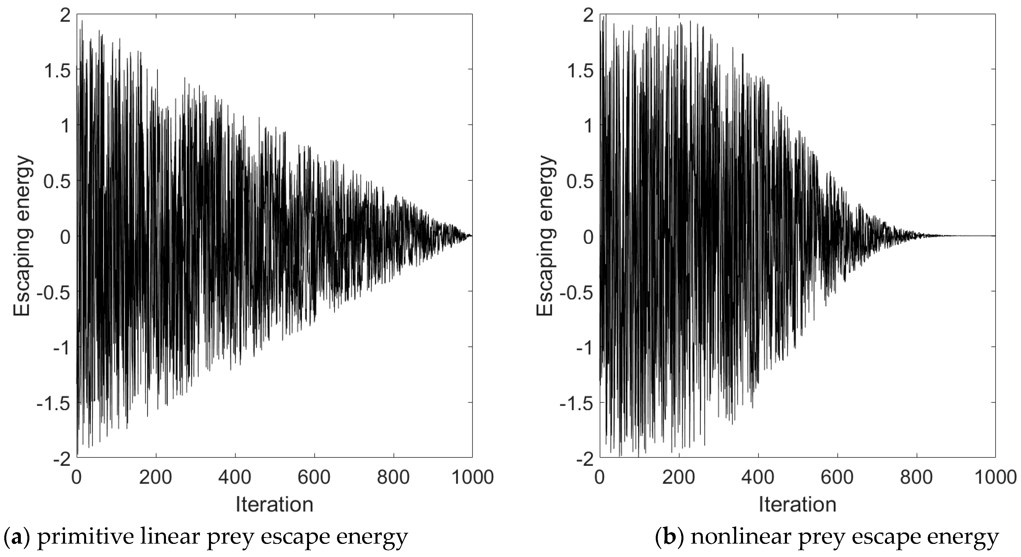
In the HHO algorithm, the prey’s energy is an essential parameter to guide the update of the position of the particle. Its original escape energy is shown in Equation (4): $\mathrm{E}=2{\mathrm{E}}_0\left(1-\frac{\mathrm{t}}{\mathrm{T}}\right)$, which presents a linear feature. However, in the actual tracking process of the target, the HHO algorithm should show better search ability in the exploration phase and can locate the optimal position faster in the exploitation phase. Therefore, we construct a nonlinear function in the form of cos, which can ensure the exploration and exploitation process better, in order to achieve better convergence accuracy and improve convergence speed. The formula is:

$$\mathrm{E}=\left(2{\mathrm{E}}_0-1\right)\ast \left\{\cos \left[{\left(\frac{\mathrm{t}}{\mathrm{T}}\right)}^{\left(2-\frac{2\mathrm{t}}{\mathrm{T}}\right)}\mathsf{\pi }\right]+1\right\}$$

(28)

where $\mathrm{t}$ is the current iteration and $\mathrm{T}$ is the total iteration number.

The comparison of the proposed nonlinear energy with the original linear energy diagram is shown in Figure 3. Moreover, it is verified on the functions F1 and F21 mentioned in the literature [23] under the same conditions, and the calculation time is 0.92 s, 1.35 s and 0.90 s, 1.32 s, respectively, under linear energy and nonlinear energy conditions. The results show that the nonlinear escape energy improves the calculation speed to some extent. It can be seen from Figure 3b that, compared with Figure 3a, the method has a better search ability in the exploration stage and a stronger local exploitation ability in the exploitation stage.

Figure 3. Comparison of prey escape energy.

4.5. Weight Compensation of Particles

In the HHOPF algorithm, the set of particles with weight propagated by the motion equation is the predicted particle set, which represents the predicted density function $\mathrm{p}\left({\mathrm{x}}_{\mathrm{k}}\right|{\mathrm{y}}_{\mathrm{k}-1})$. After determining that the effective number of the particles satisfies the optimization condition, iterative optimization is performed. The core idea is to use the HHO to enhance the distribution of the particles, so that the particles move along the orientation of the high-likelihood region, to increase the precision of the particle state estimation. At this time, the HHO changes each particle’s position. If the weight is not corrected, the particle set will not be $\mathrm{p}\left({\mathrm{x}}_{\mathrm{k}}\right|{\mathrm{Z}}_{\mathrm{k}-1})$, and the theoretical basis of the Bayesian filter is lost. To resolve this problem, the importance sampling method is used to resolve the weight compensation of the optimized particle. When the particle position is changed by the optimization algorithm, the weight is compensated accordingly. The corresponding formula is as follows:

$${\mathrm{R}}_{\mathrm{k}}^{\mathrm{i}}=\frac{\mathrm{p}\left({\mathrm{x}}_{\mathrm{k}}^{\mathrm{i}}|{\mathrm{y}}_{\mathrm{k}-1}\right)}{\mathrm{g}\left({\mathrm{x}}_{\mathrm{k}}^{\mathrm{i}}\right)}$$

(29)

where ${\mathrm{R}}_{\mathrm{k}}^{\mathrm{i}}$ is the weight compensation rate of the particle $\mathrm{i}$ and $\mathrm{g}\left({\mathrm{x}}_{\mathrm{k}}\right)$ is the probability density function characterized by the optimized particle set.

In the combination formula ${\mathrm{w}}_{\mathrm{k}}^{\mathrm{i}}\propto {\mathrm{w}}_{\mathrm{k}-1}^{\mathrm{i}}\frac{\mathrm{p}\left({\mathrm{y}}_{\mathrm{k}}|{\mathrm{x}}_{\mathrm{k}}^{\mathrm{i}}\right)\mathrm{p}\left({\mathrm{x}}_{\mathrm{k}}^{\mathrm{i}}|{\mathrm{x}}_{\mathrm{k}-1}^{\mathrm{i}}\right)}{\mathrm{q}\left({\mathrm{x}}_{\mathrm{k}}^{\mathrm{i}}|{\mathrm{x}}_{\mathrm{k}-1}^{\mathrm{i}},{\mathrm{y}}_{\mathrm{k}}\right)}$, the weight compensation updating formula of the optimized particles is as follows:

$${\mathrm{w}}_{\mathrm{k}}^{\mathrm{i}}\propto {\mathrm{w}}_{\mathrm{k}-1}^{\mathrm{i}}{\mathrm{R}}_{\mathrm{k}}^{\mathrm{i}}\frac{\mathrm{p}\left({\mathrm{y}}_{\mathrm{k}}|{\mathrm{x}}_{\mathrm{k}}^{\mathrm{i}}\right)\mathrm{p}\left({\mathrm{x}}_{\mathrm{k}}^{\mathrm{i}}|{\mathrm{x}}_{\mathrm{k}-1}^{\mathrm{i}}\right)}{\mathrm{q}\left({\mathrm{x}}_{\mathrm{k}}^{\mathrm{i}}|{\mathrm{x}}_{\mathrm{k}-1}^{\mathrm{i}},{\mathrm{y}}_{\mathrm{k}}\right)}\hspace{1em}{\mathrm{w}}_{\mathrm{k}}^{\mathrm{i}}\propto {\mathrm{w}}_{\mathrm{k}-1}^{\mathrm{i}}{\mathrm{R}}_{\mathrm{k}}^{\mathrm{i}}\mathrm{p}\left({\mathrm{y}}_{\mathrm{k}}|{\mathrm{x}}_{\mathrm{k}}^{\mathrm{i}}\right)$$

(30)

In this way, the particle distribution ${\{{\mathrm{x}}_{\mathrm{k}}^{\mathrm{i}},{\mathrm{w}}_{\mathrm{k}}^{\mathrm{i}}\}}_{\mathrm{i}=1}^{\mathrm{N}}$ is approximately still subject to ${\{{\mathrm{x}}_{\mathrm{k}}^{\mathrm{i}},{\mathrm{w}}_{\mathrm{k}}^{\mathrm{i}}\}}_{\mathrm{i}=1}^{\mathrm{N}}$. At this point, the Harris hawks optimization algorithm does not modify the probability model, only optimizes the quality of the samples, theoretically ensuring the recursive framework of the Bayesian filter. And the description of the target state weights is more accurate.

4.6. The Proposed Algorithm

The research provides a new method for underwater target tracking by particle filter. The underwater visual object tracking structure of the proposed Harris hawks optimized particle filter is shown in the flow chart of Figure 4, which shows the overall logic and steps of the HHOPF tracking.

Figure 4. Flowchart of the proposed HHOPF tracking method.

First, we can obtain the overall data set containing the tracking target. Then, the real location of the initial frame target is generally given, and its features are extracted to build our observation model. After that, we first identify the target and initialize it, and perform corrected background-weighted histogram processing to reduce the background information and to continuously track the object in the remaining image frames. Before tracking, the observation model initializes particles (number of particles N) as candidates and assigns weight to each candidate particle object. Moreover, each candidate particle has its state path and moves via the motion model. In the subsequent trace, the particle weights are updated using the Bhattacharyya coefficient. It is common to use the Bhattacharyya coefficient to compare the two histograms, as shown in Equation (31):

$$\mathrm{B}\left({\mathrm{h}}_1,{\mathrm{h}}_2\right)=1-\sum _{\mathrm{i}=1}^{\mathrm{n}}\sqrt{{\mathrm{h}}_1\left(\mathrm{i}\right){\mathrm{h}}_2\left(\mathrm{i}\right)}$$

(31)

where ${\mathrm{h}}_1$ and ${\mathrm{h}}_2$ are associated histograms. When the histograms of ${\mathrm{h}}_1$ and ${\mathrm{h}}_2$ are similar, the results of $\mathrm{B}\left({\mathrm{h}}_1,{\mathrm{h}}_2\right)$ are significant.

To solve the sample impoverishment problem in the particle filter, we use the improved HHO algorithm built with nonlinear energy to optimize the particles before resampling them, so that the particles shift towards the high probability density area. After that, all particle states are weighted-sum and a new weight is assigned to the particles to measure the new target state in subsequent frames. Object tracking is improved by increasing or decreasing the Bhattacharyya coefficient $\mathrm{B}\left({\mathrm{h}}_1,{\mathrm{h}}_2\right)$. The tracing process is complete from the first frame until all available frames are completed.

5. Experimental Results and Discussion

In this section, we begin with a brief representation of the experimental environment. After that, we express the criteria to judge the tracking performance and analyze the performance of the proposed tracking algorithm under different constraints. The details are discussed below.

5.1. Experiment Settings

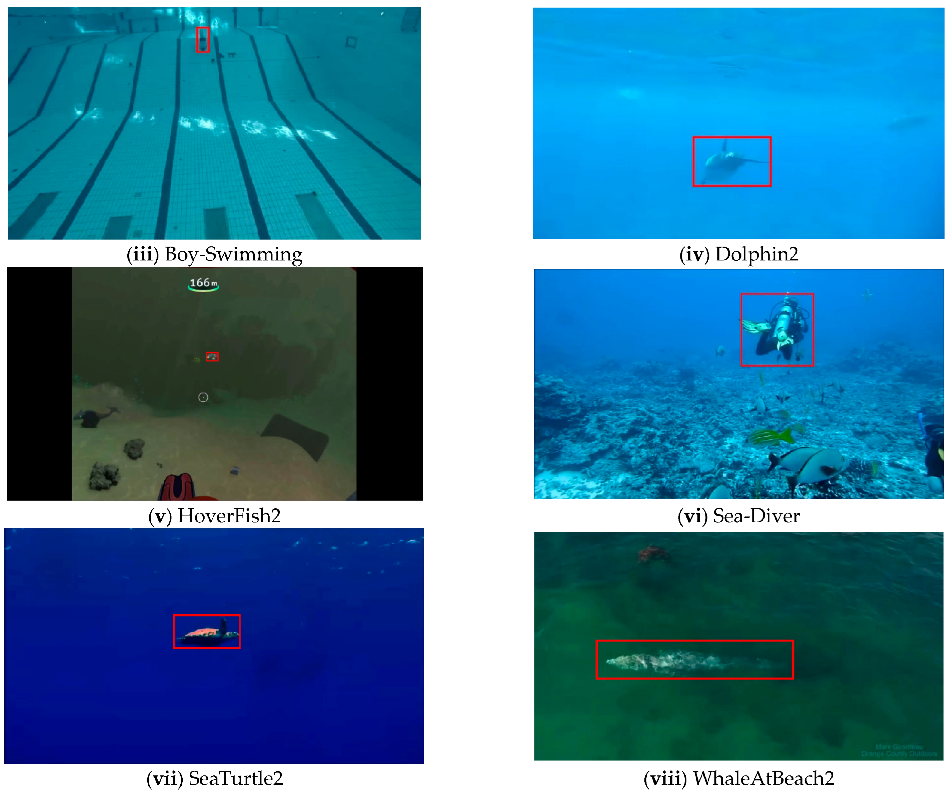
To evaluate the HHOPF algorithm, we conducted experiments using part of the reference data sets in UOT100 (Note: the datasets were obtained from the website https://www.kaggle.com/datasets/landrykezebou/uot100-underwater-object-tracking-dataset, accessed on 1 December 2022). Table 1 shows some information about the data sets. Figure 5 shows some snapshots of these data sets. The experiments were conducted using MATLAB R2020a on the following machines: Intel (R) Core (TM) i5-9300H CPU @ 2.40 GHz, 8.00 GB RAM (Note: the manufacturer's name is Hewlett-Packard (HP), USA).

Table 1. Trace sample properties.

Datasets	Frame Numbers	Challenging Factors
Little-Monster	583	Scale Variation, Deformation, In-Plane Rotation, Background Clutter
BlueFish2	593	Scale Variation, Occlusion, Deformation, In-Plane Rotation, Background Clutter
Boy-Swimming	648	Illumination Variation, Scale Variation, Deformation
Dolphin2	390	Illumination Variation, Scale Variation, Deformation, Occlusion, In-Plane Rotation
HoverFish2	449	Scale Variation, Deformation, Low Resolution, In-Plane Rotation
Sea-Diver	818	Scale Variation, Deformation, Background Clutter
SeaTurtle2	823	Scale Variation, Deformation, In-Plane Rotation
WhaleAtBeach2	317	Illumination Variation, Scale Variation, In-Plane Rotation, Background Clutter

Figure 5. Sequence of images used for visual tracking evaluation.

5.2. Use Other Advanced Methods for Evaluation

By associating the HHOPF algorithm with other evolution-based methods (PF, PSOPF, FAPF [25], SMOPF), the strength of the HHOPF tracker was evaluated. We further explained the tracking performance of the HHOPF by comparing it with other contemporary advanced tracking methods: Adaptive spatial regularization correlation filter (ASRCF) [26], Spatial-temporal regularized correlation filters (STRCF) [27], Automatic spatio-temporal regularization (Auto-Track) [28], Unsupervised deep tracking (UDT) [29], Occlusion-aware real-time object tracking (ROT) [30], Multi-cue correlation filters (MCCT) [31], and Aberrance repressed correlation filters (ARCF) [32].

5.3. Qualitative and Quantitative Analysis

Each data set in the UOT100 is affected by more than a single factor and has numerous challenging factors. We evaluated the tracking method in terms of data challenges. First, after analyzing and comparing the HHOPF tracker with the other proposed evolution-based methods, our tracker is superior to other trackers in facing various difficulties, as shown in Figure 6.

Figure 6. Different tracking in video sequence set (Little-Monster, BlueFish2. Boy-Swimming, Dolphin2, HoverFish2, Sea-Diver, SeaTurtle2, WhaleAtBeach2) tracking results.

In the face of background clutter and scaling, for example, with BlueFish2 and WhaleAtBeach2, the proposed algorithm can quickly relocate the target position after background clutter occurs, but other algorithms may fail to track the target due to the influence of incorrect background information. Another example is in the case of rapid movement in the Little-Monster data set. After setting the unified equation of motion, it can be found that the presented method can track the object in all frames, but other methods cannot keep track of the target. The main reason is that, in the process of the target’s rapid movement due to the continuous introduction of extra background information, although it can roughly track the target, the overall tracking result is not excellent. In the last example, in the Sea-Diver data set, the main problems include the slight target deformation and scale change, as well as the background interference in the short frames. In the beginning, all the comparison methods can track the target correctly, but when the target has a slight deformation, the tracking algorithm changes the tracking box accordingly due to the extracted feature information. Among them, FAPF makes the tracking box shrink accordingly due to the extracted information, while SMOPF makes the tracking box expand to a certain extent. After that, the information stored in the tracking box leads to errors in the subsequent tracking results. In the final result, it can be found that, although the tracking box of the comparison method contains the target, there will be a large error in the accuracy, while the tracking box of the presented algorithm is relatively closer to the real box size. The results of the study in Figure 6 show that the HHOPF method is better than other comparative evolution-based methods.

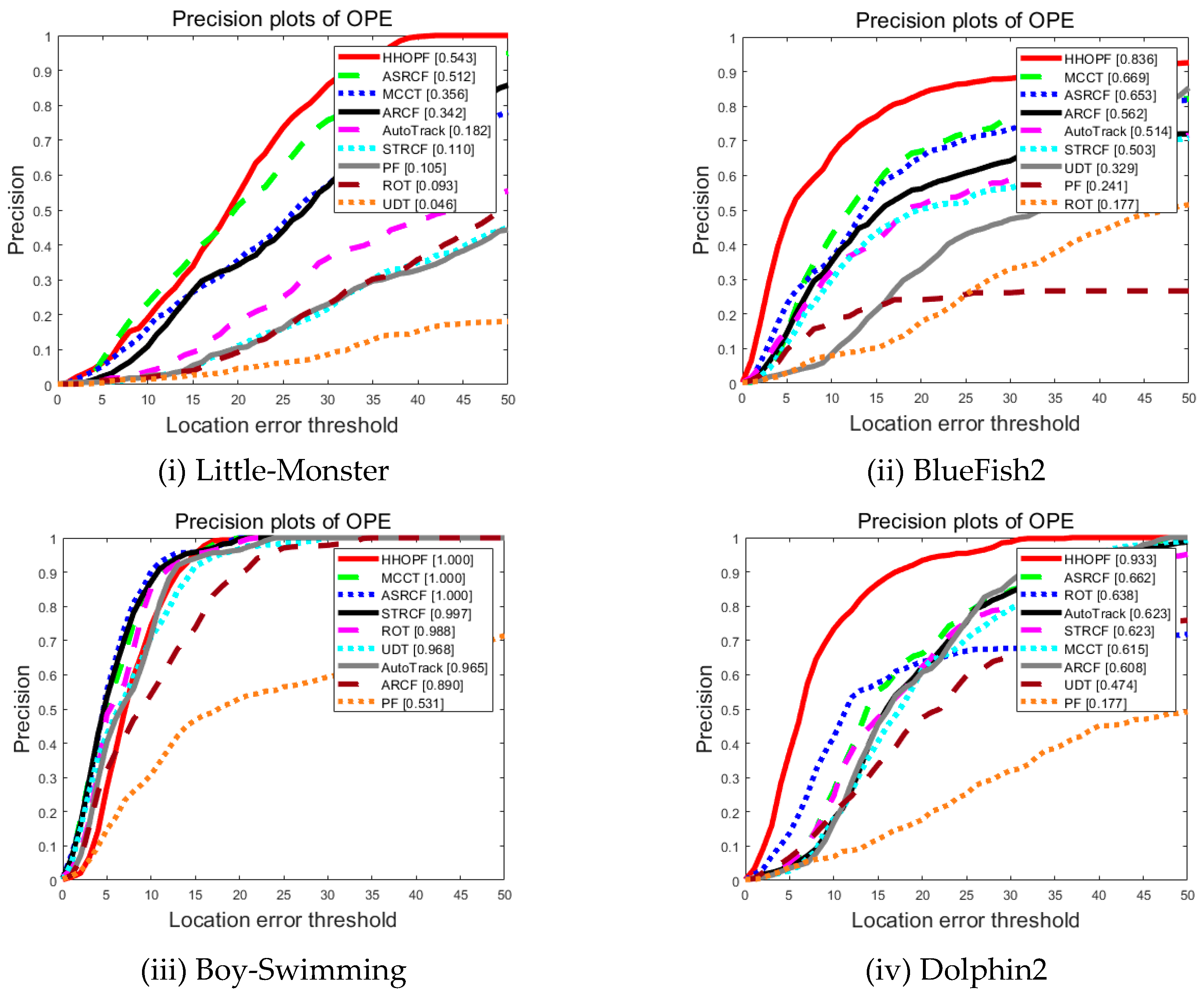
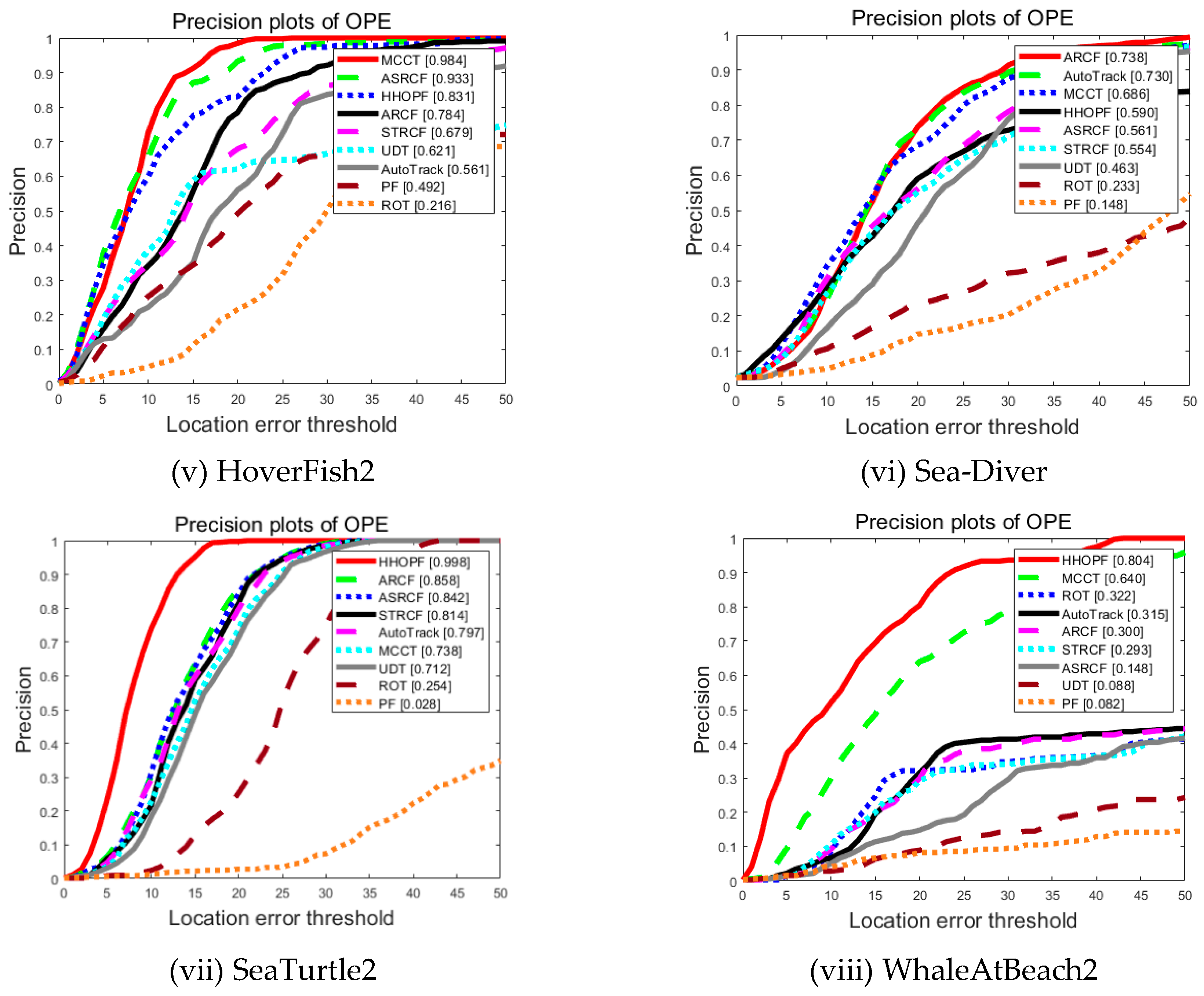
In this paper, we use tracking accuracy and overlap accuracy to correlate the proposed HHOPF tracking method with other advanced tracking techniques from recent years. Equation (32) defines the central error, and the tracking accuracy is defined as Equation (33):

$$\mathrm{C}\mathrm{L}\mathrm{E}\left(\mathrm{t}\right)=\sqrt{{\left({\mathrm{x}}_{\mathrm{T}}^{\mathrm{t}}-{\mathrm{x}}_{\mathrm{G}}^{\mathrm{t}}\right)}^2-{\left({\mathrm{y}}_{\mathrm{T}}^{\mathrm{t}}-{\mathrm{y}}_{\mathrm{G}}^{\mathrm{t}}\right)}^2}$$

(32)

$$\mathrm{D}\mathrm{P}\left(\mathrm{t}\right)=\frac{{\sum }_{\mathrm{t}=1}^{\mathrm{n}}\mathrm{C}\mathrm{o}\mathrm{u}\mathrm{n}\mathrm{t}\left[\mathrm{C}\mathrm{L}\mathrm{E}\left(\mathrm{t}\right)<20\right]}{\mathrm{n}}$$

(33)

where $({\mathrm{x}}_{\mathrm{G}}^{\mathrm{t}},{\mathrm{y}}_{\mathrm{G}}^{\mathrm{t}})$ expresses the true center position of the target box, $({\mathrm{x}}_{\mathrm{T}}^{\mathrm{t}},{\mathrm{y}}_{\mathrm{T}}^{\mathrm{t}})$ expresses the center position of the proposed tracking algorithm obtained, t is the current frame, and n is the total frames.

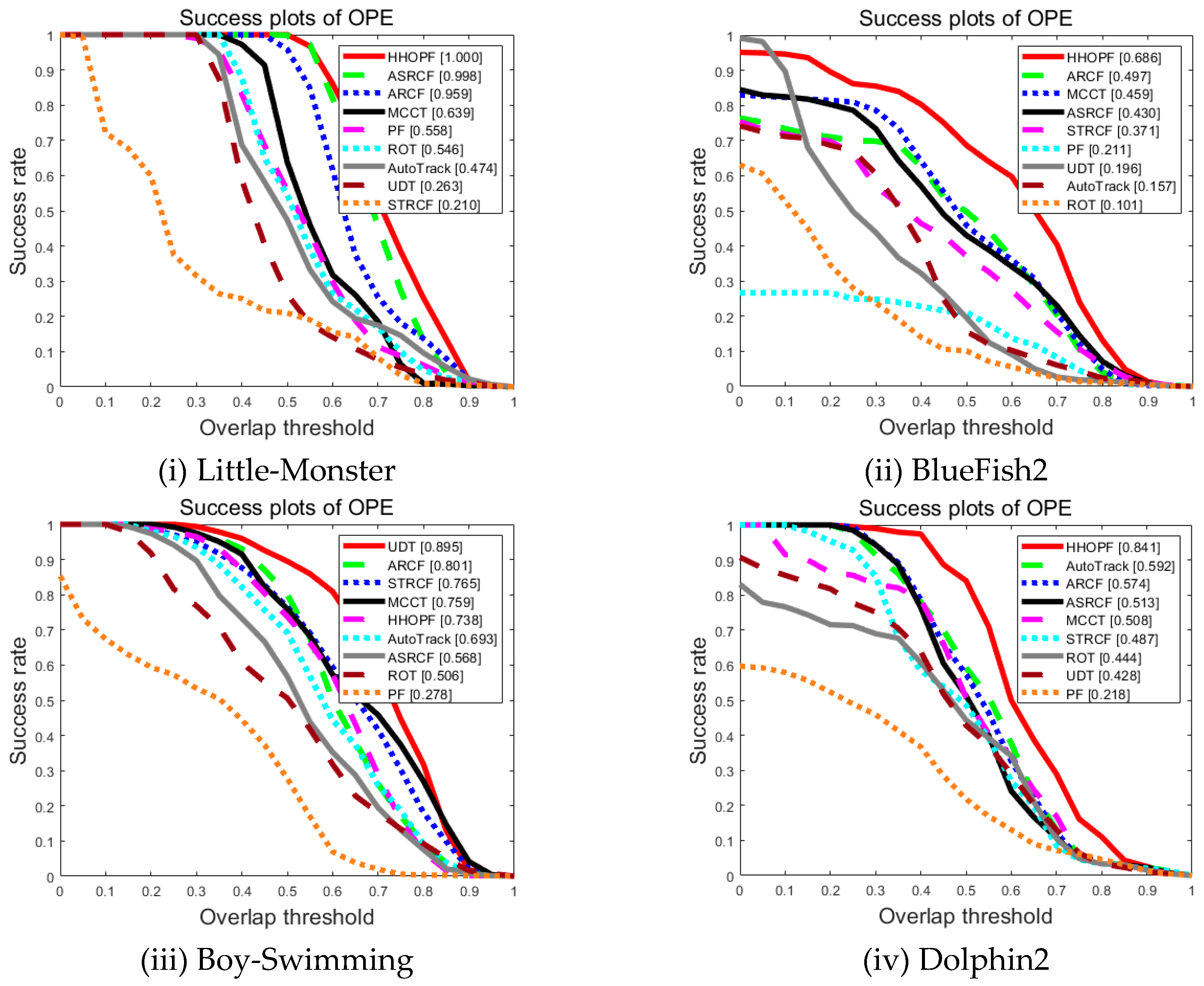
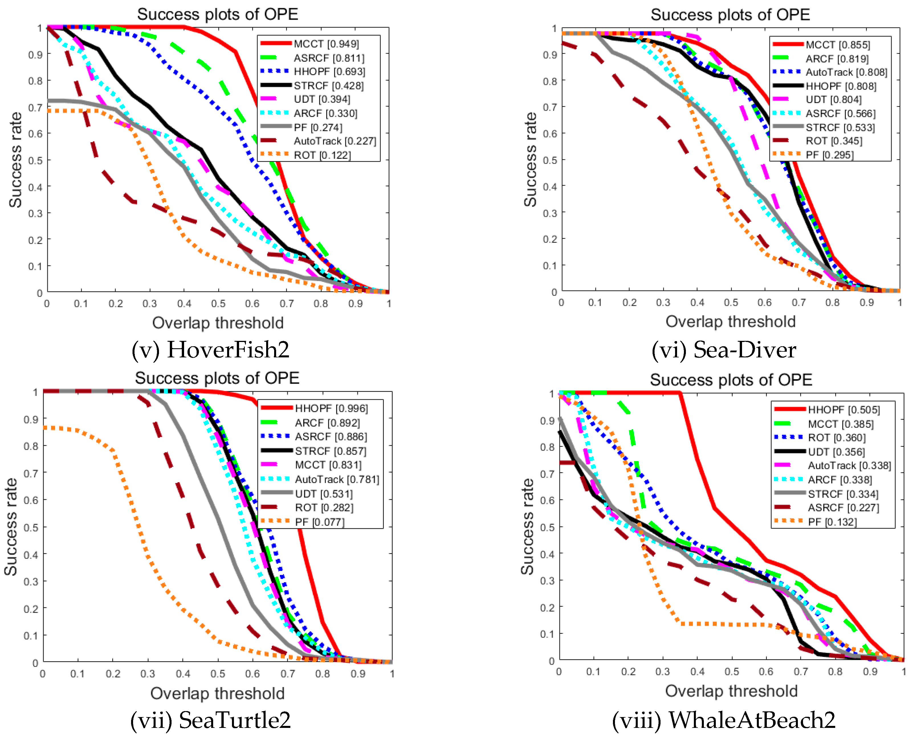
The tracking accuracy is the proportion of frames with a center location error of less than 20 pixels in the sequence data set. Table 2 shows the tracking accuracy of these trackers. We can see that the best trackers are expected to have a small central error value. In addition, we also use overlap accuracy to evaluate the proposed tracking algorithm and its competing trackers. The overlap rate between the predicted frame and the real frame per frame is Equation (34), and the overlap accuracy is defined as Equation (35):

$$\mathrm{O}\mathrm{R}\left(\mathrm{t}\right)=\frac{\mathrm{a}\mathrm{r}\mathrm{e}\mathrm{a}\left({\mathrm{R}}_{\mathrm{T}}^{\mathrm{t}}\cap {\mathrm{R}}_{\mathrm{G}}^{\mathrm{t}}\right)}{\mathrm{a}\mathrm{r}\mathrm{e}\mathrm{a}\left({\mathrm{R}}_{\mathrm{T}}^{\mathrm{t}}\cup {\mathrm{R}}_{\mathrm{G}}^{\mathrm{t}}\right)}$$

(34)

$$\mathrm{O}\mathrm{P}\left(\mathrm{t}\right)=\frac{{\sum }_{\mathrm{i}=1}^{\mathrm{n}}\mathrm{C}\mathrm{o}\mathrm{u}\mathrm{n}\mathrm{t}\left[\mathrm{O}\mathrm{R}\left(\mathrm{i}\right)>0.5\right]}{\mathrm{n}}$$

(35)

where ${\mathrm{R}}_{\mathrm{G}}^{\mathrm{t}}$ represents the boundary box of the real situation of the target object, and ${\mathrm{R}}_{\mathrm{T}}^{\mathrm{t}}$ expresses the boundary box of the forecast situation of the target object in frame t. The overlap accuracy generally refers to the proportion of frames whose intersection ratio is greater than 0.5. Table 3 summarizes the overlap accuracy of these trackers.

Table 2. Comparison results in terms of tracking accuracy.

	ROT	Auto-Track	ASRCF	MCCT	STRCF	UDT	ARCF	PF	HHOPF
Little-Monster	0.093	0.182	0.512	0.356	0.110	0.046	0.342	0.105	0.543
BlueFish2	0.177	0.514	0.653	0.669	0.503	0.329	0.562	0.241	0.836
Boy-Swimming	0.988	0.965	1.000	1.000	0.997	0.968	0.890	0.531	1.000
Dolphin2	0.638	0.623	0.662	0.615	0.623	0.474	0.608	0.177	0.933
HoverFish2	0.216	0.561	0.933	0.984	0.679	0.621	0.784	0.492	0.831
Sea-Diver	0.233	0.730	0.561	0.686	0.554	0.463	0.738	0.148	0.590
SeaTurtle2	0.254	0.797	0.842	0.738	0.814	0.712	0.858	0.028	0.998
WhaleAtBeach2	0.322	0.315	0.148	0.640	0.293	0.088	0.300	0.082	0.804

Table 3. Comparison results in terms of overlap accuracy.

	ROT	Auto-Track	ASRCF	MCCT	STRCF	UDT	ARCF	PF	HHOPF
Little-Monster	0.546	0.474	0.998	0.639	0.210	0.263	0.959	0.558	1.000
BlueFish2	0.101	0.157	0.430	0.459	0.371	0.196	0.497	0.211	0.686
Boy-Swimming	0.506	0.693	0.568	0.759	0.765	0.895	0.801	0.278	0.738
Dolphin2	0.444	0.592	0.513	0.508	0.487	0.428	0.574	0.218	0.841
HoverFish2	0.122	0.227	0.811	0.949	0.428	0.394	0.330	0.274	0.693
Sea-Diver	0.345	0.808	0.566	0.855	0.533	0.804	0.819	0.295	0.808
SeaTurtle2	0.282	0.781	0.886	0.831	0.857	0.531	0.892	0.077	0.996
WhaleAtBeach2	0.360	0.338	0.227	0.385	0.334	0.356	0.338	0.132	0.505

We indicate the best result in red during tracking and indicate the second-best result in blue. The data in Table 2 and Table 3 show that our tracker has a good tracking result. Figure 7 and Figure 8 show the schematics of the tracking accuracy and overlap accuracy of different underwater tracking sequence sets.

Figure 7. Schematic diagram of tracking accuracy of different sequences (Little-Monster, BlueFish2, Boy-Swimming, Dolphin2, HoverFish2, Sea-Diver, SeaTurtle2, WhaleAtBeach2).

Figure 8. Schematic diagram of overlapping accuracy of different sequences (Little-Monster, BlueFish2, Boy-Swimming, Dolphin2, HoverFish2, Sea-Diver, SeaTurtle2, WhaleAtBeach2).

Table 4 shows the calculation time between our proposed HHOPF algorithm and the PF, FAPF, PSOPF, and SPMOPF. The table shows that our calculation time is lower than other methods, and the HHOPF algorithm can realize real-time tracking.

Table 4. Calculation time.

Dataset	Average Computational Cost (ms)
	PF	FAPF	PSOPF	SMOPF	HHOPF
Boy-Swimming	37.34	39.64	47.54	39.21	36.22
Dolphin2	24.60	24.66	24.12	31.95	24.87
SeaTurtle2	43.59	47.46	49.02	47.43	42.49
WhaleAtBeach2	30.05	36.37	31.03	45.04	37.70

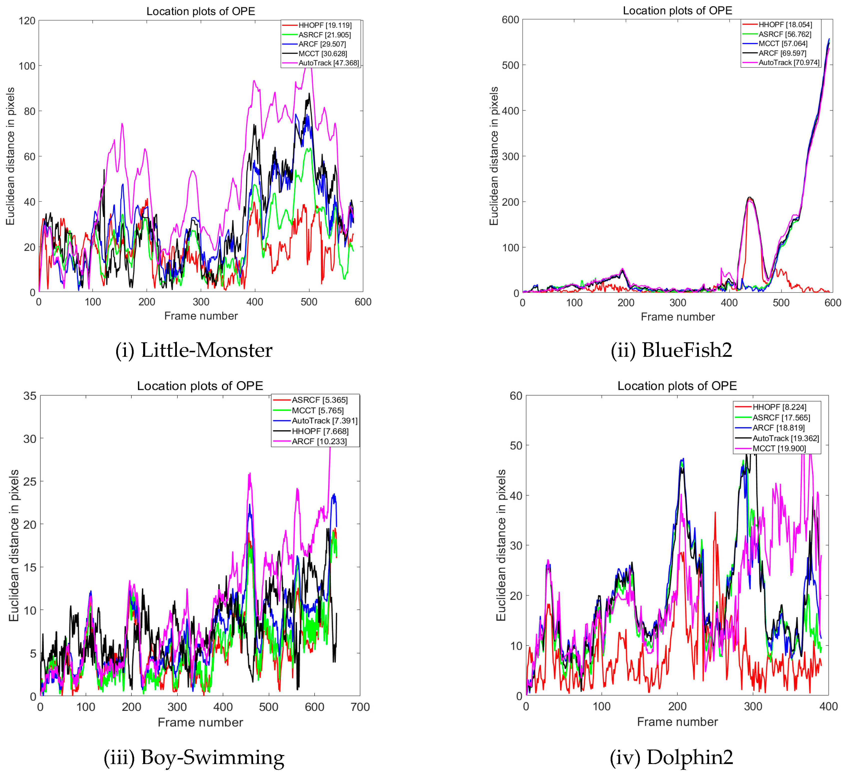
A similar observation is also shown in Figure 9, which expresses the center location errors on the sequence set between the groups of methods (ASRCF, ARCF, MCCT, Auto-Track) with better comparison results and the proposed method (HHOPF). In the tracking process of BlueFish2, the second sequence set shown in Figure 9, the targets before the 70 frame kept moving to the left, the scale change was not obvious, and the moving speed was relatively uniform. All the trackers could maintain a good result. However, at frame 70, the target performed a change in the in-plane rotation, and the MCCT algorithm produced a certain position prediction deviation. Thanks to the timely updating of the observation information in the follow-up tracking, the follow-up tracking results were guaranteed. In the following 70 to 420 frames, the tracking target mainly had challenges such as partial deformation, scale transformation, and partial occlusion. The figure shows that the tracking results of the above five algorithms can still maintain a good result. In frame 420, the effect of background clutter occurred. Subsequently, we found that, although the ASRCF and MCCT showed the tracking target in the figure, they had lost the tracking target when the target moved out of the background clutter area. However, the HHOPF, ARCF, and Auto-Track were affected when the background clutter occurred, but the algorithm proposed by us could quickly correct back and successfully perform subsequent operations, while the remaining four methods failed to track the target on the subsequent frames.

Figure 9. Central location errors of different sequence sets (Little-Monster, BlueFish2, Boy-Swimming, Dolphin2).

Through the above results in the UOT100 partial data set, the proposed algorithm has achieved satisfactory results. Not only has the tracking performance considerably improved compared with other evolution-based particle filters, but it can also comprehensively achieve better results compared with the current advanced trackers, and maintain a certain competitiveness. After analyzing the results under the different challenge factors, the proposed algorithm has a good performance on the challenge factors of scale change and short-time occlusion. In the face of fast motion and long-term occlusion problems, our algorithm has some room for improvement.

6. Conclusions

In this paper, a new evolution-based particle filter, HHOPF, is introduced for underwater visual tracking. A particle filter suffers from the traditional problem of repeated sampling, which hurts the diversity of the particles and rapidly leads to the problem of sample impoverishment. It affects the tracking performance of underwater targets. By pointing this out, we combine the particle filter with the Harris hawks optimization algorithm. In the beginning, to make the feature information of underwater target tracking accurate, the corrected background-weighted histogram was combined to construct the target feature, which reduced the background information and provided a better observation model. Then, the tracking performance of the algorithm was further improved by using the nonlinear escape energy function in the HHO algorithm to better balance the exploration and exploitation process. In addition, the particles were used to model the specific search and exploitation processes, and these functions adapted to the high-likelihood region. At the same time, the obtained state value of the particle target was introduced into the scale filter to resolve the scale change problem better and more accurately. Finally, the presented HHOPF tracker was validated by using the UOT100 data set to study its tracking performance in various environments. The experimental results showed that the HHOPF has abundant advantages in tracking, and the tracking accuracy and overlap accuracy were improved by 11% compared with other algorithms. In future work, we will apply our proposed HHOPF to the actual environment with more challenging factors, and improve the algorithm to study the problem of underwater multi-target tracking.

References

1. Sharma, K.D.; Chatterjee, A.; Rakshit, A. A PSO–Lyapunov Hybrid Stable Adaptive Fuzzy Tracking Control Approach for Vision-Based Robot Navigation. IEEE Trans. Instrum. Meas. 2012, 61, 1908–1914. [Google Scholar] [CrossRef]
2. Kim, S.H.; Choi, H.L. Convolutional Neural Network-Based Multi-Target Detection and Recognition Method for Unmanned Airborne Surveillance Systems. Int. J. Aeronaut. Space Sci. 2019, 20, 1038–1046. [Google Scholar] [CrossRef]
3. Park, H.; Ham, S.-H.; Kim, T. Object Recognition and Tracking in Moving Videos for Maritime Autonomous Surface Ships. J. Mar. Sci. Eng. 2022, 10, 841. [Google Scholar] [CrossRef]
4. Hua, X.; Cui, X.; Xu, X. Underwater object detection algorithm based on feature enhancement and progressive dynamic aggregation strategy. Pattern Recognit. 2023, 139, 109511. [Google Scholar] [CrossRef]
5. Song, P.; Li, P.; Dai, L. Boosting R-CNN: Reweighting R-CNN samples by RPN’s error for underwater object detection. Neurocomputing 2023, 530, 150–164. [Google Scholar] [CrossRef]
6. Cuan, B.; Idrissi, K.; Garcia, C. Deep Siamese Network for Multiple Object Tracking. In Proceedings of the 2018 IEEE 20th International Workshop on Multimedia Signal Processing (MMSP), Vancouver, BC, Canada, 29–31 August 2018; pp. 1–6. [Google Scholar] [CrossRef]
7. Rout, D.K.; Subudhi, B.N.; Veerakumar, T. Walsh–Hadamard-Kernel-Based Features in Particle Filter Framework for Underwater Object Tracking. IEEE Trans. Ind. Inform. 2020, 16, 5712–5722. [Google Scholar] [CrossRef]
8. Wang, X.; Wang, G.; Zhao, Z. An Improved Kernelized Correlation Filter Algorithm for Underwater Target Tracking. Appl. Sci. 2018, 8, 2154. [Google Scholar] [CrossRef]
9. Wu, X.; Han, X.; Zhang, Z. A Hybrid Excitation Model Based Lightweight Siamese Network for Underwater Vehicle Object Tracking Missions. J. Mar. Sci. Eng. 2023, 11, 1127. [Google Scholar] [CrossRef]
10. Hong, X.; Cui, B.; Chen, W. Research on Muti-Ship Target Detection and Tracking Method Based on Camera in Complex Scenes. J. Mar. Sci. Eng. 2022, 10, 978. [Google Scholar] [CrossRef]
11. Dou, J.F.; Li, J.X. Robust visual tracking base on adaptively multi-feature fusion and particle filter. Optik 2014, 125, 1680–1686. [Google Scholar] [CrossRef]
12. Dai, Y.; Liu, B. Robust video object tracking via Bayesian model averaging-based feature fusion. Opt. Eng. 2016, 55, 083102. [Google Scholar] [CrossRef]
13. Brasnett, P.; Mihaylova, L.; Bull, D. Sequential Monte Carlo tracking by fusing multiple cues in video sequences. Image Vis. Comput. 2007, 25, 1217–1227. [Google Scholar] [CrossRef]
14. Wang, Z.; Liu, Z.; Liu, W. Particle filter algorithm based on adaptive resampling strategy. In Proceedings of the 2011 International Conference on Electronic & Mechanical Engineering and Information Technology, Harbin, China, 12–14 August 2011; Volume 6, pp. 3138–3141. [Google Scholar] [CrossRef]
15. Li, L.; Ji, H.; Luo, J. The iterated extended Kalman particle filter. In Proceedings of the IEEE International Symposium on Communications and Information Technology, Beijing, China, 12–14 October 2005; Volume 2, pp. 1213–1216. [Google Scholar] [CrossRef]
16. Zhou, Z.; Yang, X.; Ji, H. Improving the classification accuracy of fishes and invertebrates using residual convolutional neural networks. ICES J. Mar. Sci. 2023, 80, 1256–1266. [Google Scholar] [CrossRef]
17. Zhou, Z.; Liu, D.; Wang, Y. Illumination correction via optimized random vector functional link using improved Harris hawks optimization. Multimed. Tools Appl. 2022, 81, 25007–25027. [Google Scholar] [CrossRef]
18. Zhou, Z.; Yang, X.; Zhu, Z. Color constancy with an optimized regularized random vector functional link based on an improved equilibrium optimizer. J. Opt. Soc. Am. A 2022, 39, 482–493. [Google Scholar] [CrossRef]
19. Zhong, J.; Fung, Y.; Dai, M. A biologically inspired improvement strategy for particle filter: Ant colony optimization assisted particle filter. Int. J. Control Autom. Syst. 2010, 8, 519–526. [Google Scholar] [CrossRef]
20. Liang, X.; Feng, J.; Li, Q. A swarm Intelligence Optimization for Particle Filter. In Proceedings of the 2008 7th World Congress on Intelligent Control and Automation, Chongqing, China, 25–27 June 2008; pp. 1986–1991. [Google Scholar] [CrossRef]
21. Rohilla, R.; Sikri, V.; Kapoor, R. Spider monkey optimisation assisted particle filter for robust object tracking. IET Comput. Vis. 2017, 11, 207–219. [Google Scholar] [CrossRef]
22. Nenavath, H.; Ashwini, K.; Jatoth, R.K. Intelligent Trigonometric Particle Filter for visual tracking. ISA Trans. 2022, 128, 460–476. [Google Scholar] [CrossRef]
23. Heidari, A.A.; Mirjalili, S.; Faris, H. Harris hawks optimization: Algorithm and applications. Future Gener. Comput. Syst. 2019, 97, 849–872. [Google Scholar] [CrossRef]
24. Danelljan, M.; Häger, G.; Felsberg, M. Accurate Scale Estimation for Robust Visual Tracking. In Proceedings of the British Machine Vision Conference, Nottingham, UK, 1–5 September 2014. [Google Scholar] [CrossRef]
25. Gao, M.; Li, L.; Sun, X. Firefly algorithm (FA) based particle filter method for visual tracking. Optik 2015, 126, 1705–1711. [Google Scholar] [CrossRef]
26. Dai, K.; Wang, D.; Lu, H. Visual Tracking via Adaptive Spatially-Regularized Correlation Filters. In Proceedings of the IEEE/CVF Conference on Computer Vision and Pattern Recognition, Long Beach, CA, USA, 15–20 June 2019; pp. 4665–4674. [Google Scholar] [CrossRef]
27. Li, F.; Tian, C.; Zuo, W. Learning Spatial-Temporal Regularized Correlation Filters for Visual Tracking. In Proceedings of the IEEE/CVF Conference on Computer Vision and Pattern Recognition, Salt Lake City, UT, USA, 18–23 June 2018; pp. 4904–4913. [Google Scholar] [CrossRef]
28. Li, Y.; Fu, C.; Ding, F. Auto-Track: Towards High-Performance Visual Tracking for UAV With Automatic Spatio-Temporal Regularization. In Proceedings of the 2020 IEEE/CVF Conference on Computer Vision and Pattern Recognition, Seattle, WA, USA, 13–19 June 2020; pp. 11920–11929. [Google Scholar] [CrossRef]
29. Wang, N.; Song, Y.; Ma, C. Unsupervised Deep Tracking. In Proceedings of the 2019 IEEE/CVF Conference on Computer Vision and Pattern Recognition, Long Beach, CA, USA, 15–20 June 2019; pp. 1308–1317. [Google Scholar] [CrossRef]
30. Dong, X.; Shen, J.; Yu, D. Occlusion-Aware Real-Time Object Tracking. IEEE Trans. Multimed. 2017, 19, 763–771. [Google Scholar] [CrossRef]
31. Wang, N.; Zhou, W.; Tian, Q. Multi-cue Correlation Filters for Robust Visual Tracking. In Proceedings of the 2018 IEEE/CVF Conference on Computer Vision and Pattern Recognition, Salt Lake City, UT, USA, 18–23 June 2018; pp. 4844–4853. [Google Scholar] [CrossRef]
32. Huang, Z.; Fu, C.; Li, Y. Learning Aberrance Repressed Correlation Filters for Real-Time UAV Tracking. In Proceedings of the 2019 IEEE/CVF International Conference on Computer Vision, Seoul, Republic of Korea, 27 October–2 November 2019; pp. 2891–2900. [Google Scholar] [CrossRef]
Disclaimer/Publisher’s Note: The statements, opinions and data contained in all publications are solely those of the individual author(s) and contributor(s) and not of MDPI and/or the editor(s). MDPI and/or the editor(s) disclaim responsibility for any injury to people or property resulting from any ideas, methods, instructions or products referred to in the content.
Article Metrics
Citations
Article Access Statistics
Multiple requests from the same IP address are counted as one view.