Abstract
For some highly nonlinear problems, the general second-order response surface method (RSM) cannot satisfy the accuracy requirement. To improve accuracy, the highest order number has to be determined in advance. Thus, a progressive trigonometric mixed response surface method (PTMRSM) was proposed to enhance the approximation accuracy and define the highest order number, rather than determining it in advance. After that, a double-loop interval optimization process could be constructed using this PTMRSM to save time while maintaining accuracy when compared to other experimental or computational methods. Unfortunately, the traditional double-loop interval optimization method had issues with the probability of reliable constraints. Then, for the construction of this double-loop interval optimization process, the modified reliable constraints were introduced. A more reliable and effective double-loop interval optimization was introduced for addressing practical engineering problems using the effective approximate method of the PTMRSM and the amended reliable constraints. Two numerical test functions and a composite submersible hull were performed to verify the accuracy and effectiveness of the PTMRSM and the double-loop interval optimization.
1. Introduction
Regarding engineering design optimization, it is usual to assess structural behavior using deterministic parameters. In practice, however, the uncertainty associated with actual parameter values is ubiquitous, ranging from simple models to complex systems. Geometric dimensions, material properties, loads, boundary conditions, manufacturing tolerance, and so on are all inherently uncertain in real-world problems [1,2,3]. Recently, a probabilistic method based on a probability density function, or distribution function, has become widely used for dealing with uncertainties. Unfortunately, it seems inevitable that there will be precise probabilistic density functions or a wealth of probabilistic data for some complicated engineering problems. Furthermore, even a small, inaccurate deviation may lead to a large error in structural problems [4,5].
To resolve this problem, a method named interval analysis was proposed by Moore [6] in the 1960s. In this book, a new interval analysis is described as neglecting the premise of a probabilistic density function or huge amounts of probabilistic data. Since then, as an efficient method, interval analysis has been used to cope with a large number of structural problems. Elishakoff and Ben-Haim [7,8] may first have applied this interval analysis as a bounded, uncertain approach for structural engineering. Qiu [5,9] employed the anti-optimization technique to solve linear interval equations for interval static displacement bounds of structures.
Nonetheless, investigating only linear programming problems in all of these reviews was an incomplete analysis since most engineering problems are nonlinear. Therefore, a nonlinear interval number programming (NINP) method is introduced to transform the uncertain optimization into deterministic multi-objective optimization using the penalty function method and the first-order Taylor expansion method introduced by Jiang [10,11,12]. It is worth noting that a large perturbation deviation of variables may cause inaccurate results in highly nonlinear systems when using the first-order Taylor expansion method for interval analysis (See Figure 1). In Figure 1, it is shown that the variation ( or ) of the first-order Taylor expansion method is obviously larger than the variation ( or ) of the actual objective function.
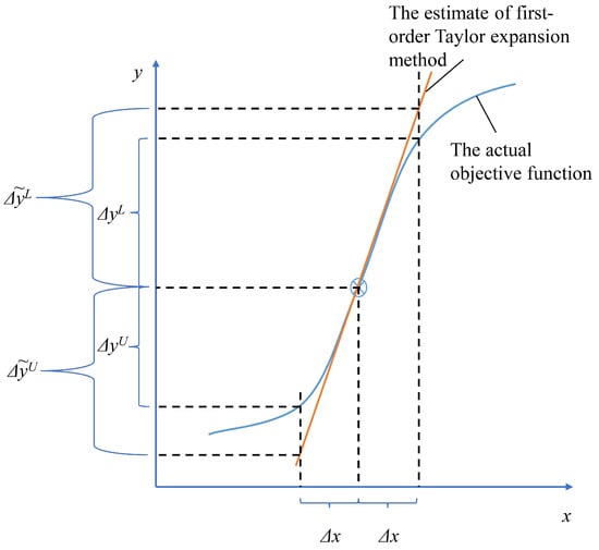
Figure 1.
The diagram of the first-order Taylor expansion estimate.
To precisely obtain more reliable results, Li et al. [3,13] formulated a nested-loop optimization procedure for engineering design optimization. Zhao [14] proposed a double-loop optimization and rebuilt the objective and constraints at each iteration step. However, the computational cost of the nested-loop optimization algorithm is always prohibitive, whether using the finite element method (FEM) or the experimental method; this may cause several weeks or months to be spent on only one optimization design [15]. To overcome this limitation of expensive computing, a surrogate model that can replace FEM or an experimental method can be expressed. Wu [1,16] developed a novel interval method for nonlinear systems based on Chebyshev polynomial series to achieve tighter and sharper bounds. Cheng [17] and Li [13] integrated the Kriging approximate model and the nested genetic algorithm to improve computational efficiency. Zhao [14] and Cheng [15] formed radial basis functions (RBF) to solve the nested interval optimization for mechanical performance. All these surrogate-based optimization methods can reduce the computational time to a few hours for one optimization design [18,19,20].
Although these surrogate models can achieve a good simulation effect, more sample points should be added to get more accurate simulation results. Basudhar [21] built a precise approximated explicit decision function based on an adaptive sample process to update this decision function. Another new sequential improvement criterion was implemented to simultaneously get the robust optimization solution and advance the suitability of the RBF proposed by Havinga [22]. Cheng [15,23] employed an adaptive Kriging model for more effective computing results by adding more sample points. Wang [24] constructed an adaptive response surface method (ARSM) that required only a reduced number of design experiments for high-dimensional engineering design problems. Chakraborty [25] performed an adaptive RSM in an iterative finite element model updating procedure that proved efficient. It is important to note that more sample points mean not only a more accurate response but also a higher computational cost. For signal classification problems, a weighted fuzzy process neural network model is proposed, and the accuracy of this method is higher than other existing automatic identification methods by S. Xu et al. [26].
Lots of methods for obtaining more precise approximations with fewer sample points have been developed and implemented. In order to construct a more efficient and accurate approximating model, Kim [27] and Youn [28] combined sensitivity information and the moving least squares method (MLSM). Kaymaz [29] and Taflanidis [30] implement a response surface model using the moving least squares method (MLSM) for the reduction of the computational burden. Li [31] proposed a doubly weighted moving least squares method, including the normal weight factor of MLSM and the distance between the most probable failure points. S. Lee [32] proposed a new approach toward reliability-based design optimization using the response surface augmented moment method (RSMM) for the progressive update of the response surface. Even though the aforementioned scholars did their best to establish an accurate surrogate model with a small number of sample points, sensitive data or other information is still needed, which can still increase computing costs.
Consequently, the trigonometric mixed response surface (TMRSM) is proposed as an updated response surface method (RSM) for obtaining perfect approximate responses in the same sample points [33]. Specifically, most of the surrogate model was constructed by the second-order polynomial [24,27,28,29,31]. Only the quadratic RSM model may be appropriate for engineering performance in some highly nonlinear cases. The conventional approach is to artificially select the order of the terms in advance, then establish this RSM function. Few papers have conducted more extensive research on the determination of high nonlinear programming for RSM. Gavin [34] introduced an algorithm process that can iteratively decide the fittest order polynomial. Along this path, this paper improved the trigonometric mixed response surface (TMRSM) to the progressive trigonometric mixed response surface (PTMRSM), which can automatically determine the order number of the surrogate model using the t-test method. Following that, a double-loop interval optimization can be built using the PTMRSM and reliable constraints. Although the possibility degree may be first introduced by C. Jiang [10] in the treatment of the interval inequality constraints, this paper fixed a minor problem with respect to this possibility degree and proposed reliable constraints in accordance with the amended possibility degree for the double-loop interval optimization.
This paper will be organized as follows. In Section 2, a novel progressive response surface method (PTMRSM) is introduced to replace the more time-consuming finite element method (FEM) and determine the order number automatically. The accuracy of the PTMRSM is verified by two general numerical test functions and one practical submersible example in Section 3. Then, a new double-loop interval optimization is proposed to improve the accuracy of interval boundaries using reliable constraints in Section 4. Finally, in Section 5, a practical submersible composite hull design is carried out to verify the efficiency of the double-loop interval optimization. The conclusion is in Section 6.
2. Progressive Trigonometric Mixed RSM (PTMSRM)
2.1. Identification of Response Surface Method
The response surface method (RSM) was originally proposed as a simple mathematical expression to express the relationship between the input and output of an experiment. Then, this effective method may be first introduced by Box and Hunter [35] and extended to other fields, especially engineering problems. The RSM function can be presented as:
in which expresses the output function; illustrates the polynomial form of ; indicates the experimental residual error, assuming that it is a normal distribution with and .
In general, approximate polynomial functions can be modeled as linear, second-order, or higher-order polynomials. Then, the common formula of the RSM model can be indicated as:
where is the actual vector of the coefficient.
2.2. Moving Least Squares Method (MLSM)
In the traditional least squares method (LSM), the response surface function is formed as:
where is a vector of polynomial basis functions, and is an evaluated vector of the coefficient. It is noted that these evaluated coefficients are constant with global regression, while changes. That is to say, the whole sample points are considered and weighted equally. However, in practical application, a precise approximated model requires greater weight on the sample points closer to the prediction point. Consequently, a weighted regression method called the moving least squares method (MLSM) is proposed to improve the coefficients . This implies that the coefficients become functions of . And the coefficients can be calculated by minimizing the residual error between the output value and the response surface value.
To construct this function, sample points of variables in the design space must be chosen based on optimal Latin hypercube design (OLHD). The output value can be calculated from these OLHD sample points using computer simulation, such as the finite element method (FEM). Once the required sample data was obtained, the polynomial constructed for all sample points can be shown as:
where can be defined as:
After that, the experimental residual error between the output value and the response surface value can be expressed as:
where can be defined as:
In Equation (6), the weight can be presented as:
where is the Euclid distance between the prediction point and the sample point, and is the influence range whose appropriate size should be selected among a sufficient number of neighboring sample points to avoid singularity in the solution. It is useful to remember that should contain at least sample points, and the weight function should vanish outside the influence range. And is the coefficient of the exponential and the Gaussian weight function. Among all the weight functions, the Gaussian function is considered to be an effective weight by most scholars for MLSM [30,31].
Figure 2 shows the shape of different weight functions using Equation (8). From Figure 2, the exponential weight function and the Gaussian weight function may have a better weight effect both in the domain range close to the sample point and away from the sample point. Nevertheless, using the exponential weight function, the weight value is not zero near the boundary of the domain area. In this regard, the Gaussian weight function may have a more suitable performance for the MLSM compared to the exponential weight function.
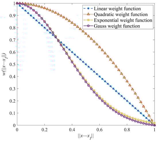
Figure 2.
The shape of different weight functions.
Figure 3 demonstrates the shape of the Gaussian weight function under different coefficients . Specifically, the value of this coefficient suggested has a nice distribution characteristic from Figure 3 [30].
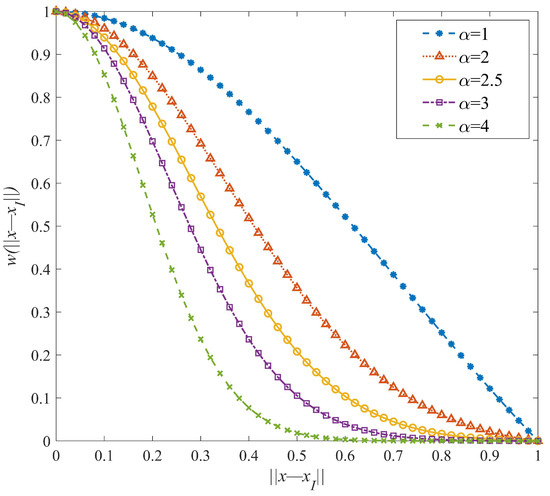
Figure 3.
The shape of Gaussian weight function under different coefficients.
The minimum of the experimental residual error can be gained by the partial derivatives with respect to coefficients, as below:
Then, the evaluated coefficient can be achieved from Equation (9):
Therefore, the contribution of the sample points will be decreased as the distance between the prediction point and is increased. This implies the MLSM can denote both a local and global approximation over the entire region.
2.3. Trigonometric Mixed Response Surface Method
Normally, the base function of the response surface method is polynomial. However, if the surrogate relationship has considerable curvature and is extremely complicated, only high-order nonlinear programming may fail to meet the accuracy requirement. For this condition, Lee and Lin [36,37] proposed a novel type of RSM to solve these complex composite problems using trigonometric functions as the basic functions. In this method, the trigonometric functions ( and ) are chosen as the basic elements to replace the traditional polynomial functions. Then, the vector of the trigonometric base functions can be presented as:
Therefore, a trigonometric mixed response surface method (TMRSM) is proposed to integrate the trigonometric functions and the MLSM based on OLHD [33].
2.4. Progressive Trigonometric Mixed Response Surface Method
Usually, most RSM models in the literature take second-order polynomials as their basic form. TMRSM, though, has successfully improved the accuracy of the surrogate model, and the determination of the higher-order polynomial should be tested in advance for the given sample data. To circumvent this deficiency, a progressive trigonometric mixed response surface method (PTMRSM) is proposed in this paper to approximate these sample points and test the necessity of the higher-order terms using a t-test.
According to Equations (4) and (10), the experimental residual error can be written as:
If , then the residual error can be abbreviated to:
Hence, the mathematical expectation and the variance can be expressed as:
where is the expectation of the evaluated coefficient . For the MLSM, the expectation of the estimated coefficient is the actual coefficient for the sample points. If , the variance of is defined as . In which the variance of is indicated as .
Furthermore, the expectation of the sum of the squared residual error is:
If the trace is simplified as , there is the variance of :
Therefore, the unbiased estimation of is:
The squared residual error can comply with , and then it can be written as . Hence, this squared residual error obeys the Chi-square distribution:
According to Equations (18) and (19), the summation of the square residual error should abide by :
From Equation (10), the mathematical expectation of this evaluated coefficient can be expressed as:
So, the variance of the evaluated coefficient can be indicated as:
Make , then we have . And a standard normal distribution can be achieved:
Combining Equations (20) and (23), the t distribution can be represented as:
where is a t-distribution of the degree of freedom.
Determining the significance of the higher-order terms means measuring the importance of these evaluated coefficients. This indicates that the insignificant coefficients stand for the unimportant higher-order terms. Equation (10) shows the vector of the coefficients, and it is easy to find the coefficient values of the highest order. Then, the focus of this work becomes to check whether the highest coefficients have significant effects on the output response. It is equivalent to whether the highest order coefficients are equal to the values of 0 (0 shows the insignificant impact). Assume a null hypothesis , and the test can be performed by calculating the t-test value.
where indicates t distribution of degree of the freedom (see Equation (24)); is the standard deviation of the coefficients; is the number of the terms of the model, which can be selected from the first number of the highest-order terms to the last number of the highest-order terms.
For this t-test, a two-sided test and 90% confidence intervals are usually chosen in this paper [34]. Then, the boundary value can be calculated by t-distribution functions. If , the null hypothesis can be rejected. This implies these coefficients and the relevant high-order terms may have a significant influence. Otherwise, the null hypothesis cannot be dismissed. That is to say, the coefficients and these high-order terms may not have a substantial effect.
In addition to the t-test criterion, other criteria should exist to ensure the relationships in which the odd or even order terms have a significant effect on the response results. Only testing whether the highest order has an important effect may easily lead to inaccurate approximations of these special functional relationships. To avoid this deficiency, the determination of the coefficient and the mean relative error should be introduced for the sample points, respectively.
where represents the sum of squares for error, which is caused by experimental error. And expresses the sum of squares for the total, representing the total variation of values of sample observations. These two values can be shown as:
where is the mean value of output response , which can be expressed as:
The determination of the coefficient is a statistical indicator that reflects the reliability of the response surface models to account for changes in terms of dependent variables. The closer this value is to 1, the better the approximated effect will be. If the determination of the coefficient for the m sample points, it means that the approximation degree is sufficient [38].
The mean relative error is another indicator that can illustrate the relative error between the actual response and the approximate response. The lesser the value is, the smaller the error is. For most practical engineering problems, it can be viewed as an appropriate limit when [38].
Eventually, another stopping criterion is the highest order limit. Given the possibility of over-fitting for the approximate functions, this model takes a stopping criterion with respect to the sixth highest order. That is due to the fact that the highest terms are really rare to exceed the fifth order for most engineering problems [34].
The proposed PTMRSM can be started with the order , and the program can determine whether the t-test values of the third-order terms are sufficient for the 90% confidence intervals. If not, the determination of the coefficient and the mean relative error will be utilized to check the reliability of the fitting performance and the relative error. If these criteria are satisfied, stop this process, and output the response. If not, continue this process until the highest order reaches the sixth order. Then, the response of PTMRSM will be outputted, displaying that “Warning: the highest order has reached the maximum value (6th order)”. Figure 4 shows the step-by-step procedure of this algorithm:
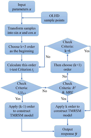
Figure 4.
The flowchart of the PTMRSM.
- Perform the OLHD sample points, and obtain the response with respect to these sample points based on FEM or specific functions;
- Transform all the sample points and the input parameters into the trigonometric functions and . Then, choose order as the beginning, and construct this third-order TMRSM;
- Calculate the values of the t-test criterion . Meanwhile, the determination of the coefficient and the mean relative error can also be calculated from Equations (28) and (29);
- Check the t-test criterion and decide whether this operation should be stopped. If the coefficients , it is concluded that the highest-order terms are insignificant. Then, stop the process, and construct the model with (k − 1)-th order TMRSM;
- If the t-test criterion is not satisfied, check the criteria for the determination of the coefficient and the mean relative error . If these criteria are fulfilled, it implies the performance and the accuracy of the approximated degree are sufficient. Then, stop this operation and build the model with k-th order TMRSM;
- Otherwise, select (k + 1)-th order as the next step order, and check whether the highest order is satisfied. If not, repeat steps 3 to step 6 until one of these criteria is satisfied;
- When the highest order is fulfilled, establish the model with the sixth order TMRSM, “Warning: the highest order number has reached the maximum value (6th order)”.
The pseudocode for the PTMRSM process is listed in the Algorithm 1.
| Algorithm 1: The pseudocode for the PTMRSM process: | |
| 1: | Read input variable matrix and output response matrix: |
| 2: | load Sample.mat; |
| 3: | Set the confidence level of t-test criterion, the determination coefficient criterion and |
| 4: | the mean relative error criterion. |
| 5: | Transform input variables and sample matrix into trigonometric functions sin θ and cos θ. |
| 6: | for sn = 1:Number of response column |
| 7: | for k = 3:6 |
| 8: | Construct the X matrix with MLSM using k order |
| 9: | Evaluated coefficient: b = (P.′ ∗ W ∗ P)\(P.′ ∗ W ∗ Y); |
| 10: | Calculate errors between actual response values and predicted values |
| 11: | Calculate the value of t-test criterion: |
| 12: | H= P *(P.′ ∗ W ∗ P)\(P.′ ∗ W); |
| 13: | s = trace((eye(m)-H) ∗ (eye(m)-H).’); |
| 14: | SSE = e.’ ∗ e; %e is the error between actual value and evaluated value |
| 15: | C_jj = diag((P.′ ∗ W ∗ P)\(P.′ ∗ W ∗ W ∗ P)/(P.′ ∗ W ∗ P)); |
| 16: | s_d = (SSE./s). ∗ C_jj; |
| 17: | tj = b./(s_d).^0.5; |
| 18: | Calculate the determination coefficient criterion value: R2 = 1-SSE./SST; |
| 19: | Calculate the mean relative error criterion value: MSE = mean(abs(e./Y)); |
| 20: | if (t < =tinv(confidence level,s) ∗ ones(highest order number,1)) |
| 21: | k = k − 1; |
| 22: | break |
| 23: | end |
| 24: | if (R2 > = 0.99)&(MSE < = 0.02) |
| 25: | k = k; |
| 26: | break |
| 27: | end |
| 28: | end |
| 29: | Adopt the new order and reconstruct the TMRSM model using updated order |
| 30: | Output the response value: |
| 31: | f (sn) = p ∗ b; |
| 32: | h_order(sn) = k; |
| 33: | sn = sn + 1; |
| 34: | end |
3. Accuracy Analysis
3.1. Numerical Rastrigin Function
The first numerical function is the well-known Rastrigin function, which can be stated as:
In this Rastrigin function, 40 sample points were designed using optimal LHD, and 100 random test points were adopted for the verification of each surrogate model. Figure 5 shows the shape function or responses of the original function, second-order RSM with MLSM, second-order TMRSM and PTMRSM under 40 sample points.
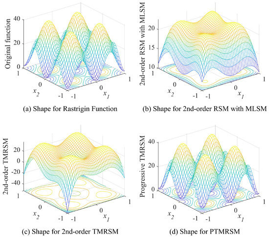
Figure 5.
The shape of different responses for Rastrigin.
It is obvious that the PTMRSM model has exactly the same shape as the original model from Figure 5a,d. Namely, the PTMRSM model has the best approximate performance in comparison with the other surrogate models. And Table 1 represents the performance and the accurate measures of each surrogate model under 100 random test points. From Table 1, it is further confirmed that the PTMRSM model has a better fitting performance and smaller mean relative error compared to other surrogate models.

Table 1.
The accuracy of different models for Rastrigin.
For the PTMRSM model, Figure 6 denotes the number of its order, which can be decided by the step-by-step procedure for 100 random test points. It can be seen that the number of orders for the PTMRSM model is third and fourth order. That implies that the highest order number is not a fixed value for PTMRSM.
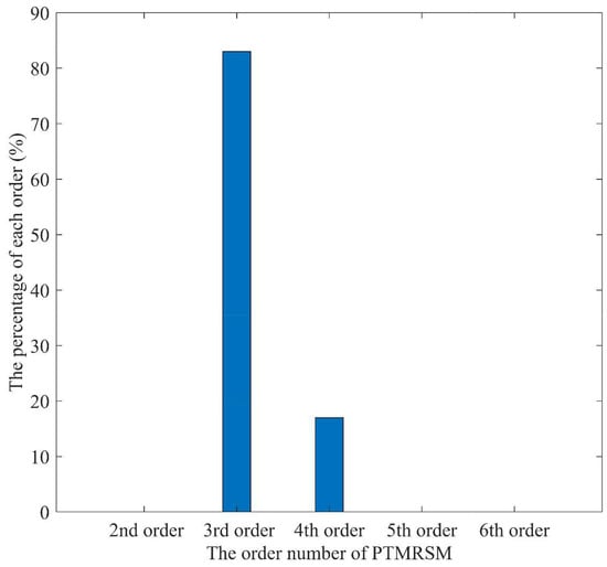
Figure 6.
The order number of PTMRSM for Rastrigin.
3.2. Numerical Example Function
The next numerical function is an example function, which has been utilized in the literature [34]. This function can be indicated below.
In this example function, there are also 40 sample points that were designed based on optimal LHD and 100 random test points that were taken to verify each surrogate model. Figure 7 expresses the shape function or responses of the original function, second-order RSM with MLSM, second-order TMRSM, and PTMRSM under 40 sample points. In this Figure, it is evident that both the PTMRSM model and the original function have almost the same shape of the response.
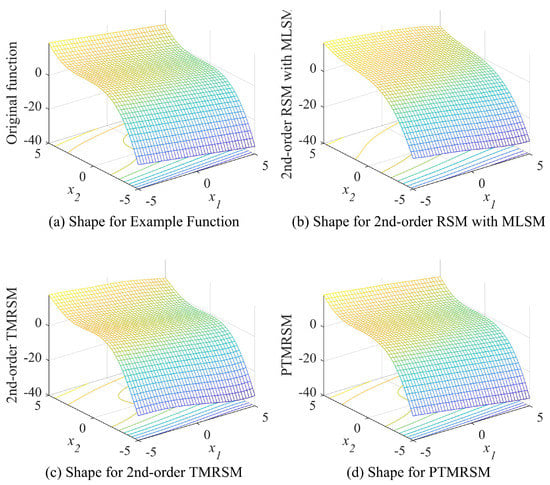
Figure 7.
The shape of different responses for an example function.
Table 2 supports the same point of view as the Rastrigin function because the PTMRSM model also has the largest and the least .
Table 2.
The accuracy of different models for an example function.
Figure 8 represents the order number of the PTMRSM model through 100 random test points. As seen, for these test points, all the highest order numbers of the constructed PTMRSM models are third order. And this means the higher order terms can improve the performance and accuracy.
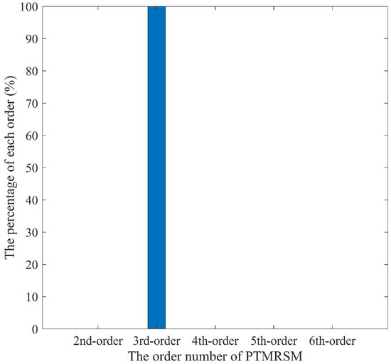
Figure 8.
The order number of PTMRSM for six hump camelback.
3.3. Composite Submersible Hull Example
In this paper, a composite submersible hull was put forward to withstand underwater pressure, whose type is the well-known Myring, as a practical example [39]. For this composite structure optimization, the stacking sequence is one of the non-trivial factors in terms of buckling performance. The conventional stacking sequence can be designed in a symmetrical form. This paper takes the symmetric type stacking sequence with a total of 10 layers, and critical buckling pressure is considered the pivotal design objective. Another design constraint can be the maximum buckling displacement for the underwater pressure. Consequently, the orientation angle of each layer can be defined as the designed vector and the thickness of the layer can be considered an uncertain factor because of the manufacturing tolerance. Figure 9 shows the diagram of the composite submersible hull.
Figure 9.
The diagram of the composite submersible hull.
Table 3 displays the performance and the accuracy of different RSM models under 100 random test points with respect to the critical buckling pressure and the maximum buckling displacement , respectively.
Table 3.
The different models for critical buckling pressure and maximum displacement.
From this table, it is obvious that the PTMRSM model has more precise results and better fitting responses than other RSM models for both the critical buckling pressure and the maximum buckling displacement.
Figure 10 and Figure 11 display the highest order distribution under 100 testing points for the critical buckling pressure and the maximum buckling displacement, respectively. For this practical submersible hull, the third-highest order is adequate in terms of both the buckling performance and the deformation performance.
Figure 10.
The order number of PTMRSM for buckling pressure.

Figure 11.
The order number of PTMRSM for buckling displacement.
4. Double-Loop Interval Optimization Method
4.1. Interval Optimization Method
Based on the interval analysis method [11,40,41], the real numbers are bounded by intervals that the interval vector can be expressed in the following form:
where and denote the lower and upper bounds, respectively; and show the center point vector and radius vector, respectively. Considering the interval vectors, the objective and constraint functions will be constructed as lower and upper intervals, respectively:
where is the design variables, and is the uncertain interval parameters.
C. Jiang performed the first-order Taylor expansion method, which is a simple approximated method for the evaluation under relatively small uncertainty [10,11,42,43].
Although this Taylor expansion method is feasible and convenient, inaccurate bounds can be obtained for high nonlinear complex structural problems under large perturbation deviations. Thus, a double-loop interval optimization method can be proposed using sequential quadratic programming (SQP) by J. Wu and F. Li [2,13,44].
In these equations, and . Similarly, the lower bound and upper bound of optimization constraints can also be written as:
With reference to Equation (35), the interval objective and constraint functions can be described as their center points and radii, respectively:
Therefore, the above interval optimal problem can be transformed into the deterministic two-objective problem below:
4.2. Reliable Constraints
To compare two interval numbers, a certain degree named possibility degree is introduced, which can convert two interval numbers into a deterministic relationship. This possibility degree may be first introduced by C. Jiang to express which interval values are larger or smaller than the other ones [28,45,46]. Figure 12 shows the whole six positional cases with respect to these two interval values and . In order to describe this deterministic relationship, the possibility degrees of the cases in Figure 12 can be displayed for ranking these two interval numbers, and , as:
Figure 12.
Six positional cases between two interval values.
For Case 2 (in Figure 12), there exist four events with respect to the two random parameters and :
However, when the event occurs, three possible events (, and ) may be encountered. An assumption that all these events have equal chance was made by P. Sevastianov [47]. That means when the event occurs, the possibility is:
Then, the conditional possibilities can be expressed as:
Consequently, the possibility of the event can be indicated as:
In Case 3 of Figure 12, there are also three possible events: , and (see Figure 13). Define three events in terms of the random parameters and in given subintervals when Case 3 appears:
Figure 13.
The diagram of possible events for Case 3. (a) , (b) and (c) .
Thus, the possibilities of , and under given event can be expressed as:
Then, the whole conditional possibilities of given , and can be indicated as:
Therefore, the probability degree of the event can be attained as:
This is a different value from Cases 2 and 3 of Equation (45). It implies C. Jiang only makes the assumption of the events and , rather than the assumption of the event of . This assumption, however, is at odds with reality. Similarly, the events in Case 4 and 5 can be illustrated, respectively, as:
So the amended possibility degree can be improved by integrating Equations (47), (51) and (55)–(57).
On the other hand, the possibility degree under the opposite rank of the two interval numbers and can be shown:
When there is an event , the possibility degrees of Cases 1 and 6 are zero. Additionally, this possibility degree is one only if and . For the condition of Case 2 and 4, the possibility degrees can be displayed, respectively, as:
Analogously, for Cases 3 and 5, the possibility degrees can be written, respectively, as:
Thus, the whole of possibility degree under the rank of event can be expressed as:
It should be mentioned that means the possibility degree level is when is smaller than . means that is always smaller than , and represents that is always larger than . Under this amended possibility degree method, the reliable constraints should fulfill a confidence degree level, and these reliable constraints are transformed into simple deterministic constraints for the double-loop interval optimization. After the premise of the possibility degree has been ensured, the simple deterministic constraints can be expressed as:
where means the interval values of constraints; and represents the relationship with regard to the constraints interval; is the number of the constraints. And can be calculated by Equations (42) and (43).
4.3. Double-Loop Interval Optimization Method
For the sake of dealing with the two-objective problem (see Equation (46)), a linear combination of the two objectives is introduced, which can be generally defined as
where is the weight values of each objective function; and are the normalization factors that can make and the same magnitude. It has to emphasize that the interval optimization problem may be either a minimization problem or a maximization problem. In this paper, the objective is a maximization issue. Consequently, the linear combination of objectives and reliable constraints can be written as:
where is the normalization factor that can make and as the same magnitude; and are the lower and upper bounds of the preset possibility degree.
In order to perform this double-loop interval optimization process, the bounds of the interval objectives and constraints should be evaluated in advance. Therefore, an inner-loop optimization should be presented to solve this min-max problem. Note that sequential quadratic programming (SQP) [3,48,49] and particle swarm optimization (PSO) [49,50] can be selected as the inner and outer optimization solvers, respectively. Figure 14 shows the flowchart of the double-loop interval optimization method.
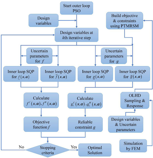
Figure 14.
The flowchart of double-loop interval optimization.
It is clear that this flowchart is a nesting double-loop interval optimization problem. The samples of design and uncertain space are performed using OLHD, and the response of these sample points can be obtained by ANSYS simulation. For the sake of saving computational cost, the aforementioned PTMRSM surrogate model can be formed as the basic objective and constraint functions instead of the more time-consuming ANSYS simulation. In the inner loop interval optimization process, SQP can be executed to compute the bounds of the inner loop objective and constraint with respect to uncertain interval vectors . Then, during the outer loop interval optimization process, PSO is carried out to optimize the linear combination objective with reliable constraints for the optimal design vector .
5. Practical Composite Submersible Hull Design
5.1. The Objective Function of the Submersible Hull Example
As mentioned above, the critical buckling pressure can be regarded as the inner loop objective function; meanwhile, the maximum buckling displacement should also be another significant effect that can be considered the inner loop constraint. In this submersible optimization design, the larger the buckling pressure is, the better the optimal solution is. Thus, the center point of the critical buckling can be treated as the maximization problem. To circumvent this problem, can be considered as one of the linear combination functions instead of . The following single-objective function with a penalty function can be formed based on the double-loop interval optimization method.
where and are center point and a radius value of the critical buckling pressure; is the possibility degree of the reliable constraint. is the weight coefficient, which can be selected as 0.5, since the center point and its radius should be minimized simultaneously. is the normalization factor with the value of 2.0 × 10⁵. is the defined maximum buckling displacement interval. is the layer thickness interval. is the outer pressure interval. and are the mean preset possibility degree level, which can be selected between 0 and 1. The larger is, the stricter the constraints will be and may lead to a narrower feasible region [10]. In this paper, a common preset possibility level can be defined as:
5.2. Results and Analysis
Table 4 shows the optimal design results of the double-loop interval optimization for the 3rd order RSM with MLSM and the PTMRSM, and the nonlinear interval number programming (NINP) method for the PTMRSM model under neutral level possibility degree. The NINP method was proposed by C. Jiang [11,42]. And this NINP method can be treated as a comparative item.
Table 4.
Optimal solution under the neutral possibility degree.
From this table, it can be seen that the double-loop interval optimization for PTMRSM has the smallest radius of the critical buckling pressure, which means the deviation of the optimal design solution can be least affected by the uncertain variables. In other words, the interval optimization for PTMRSM can obtain a more robust and reliable optimal design solution. Furthermore, the similarity between the optimal design solutions of the interval optimization for PTMRSM and the NINP method for TMRSM is greater than that of the interval optimization for 3rd-order RSM with MLSM.
Figure 15 shows the lower and the upper bounds of the critical buckling pressure for one variable orientation angle and the other four fixed orientation angles under the neutral possibility degree. Figure 15a indicates the lower and the upper bounds of the critical buckling pressure under one variable () and four invariants (, , and ). Figure 15b expresses the bounds of the critical buckling pressure under one variable () and four invariants (, , and ). Figure 15c displays the same bounds under one variable () and four invariants (, , and ). Figure 15d shows the same bounds under one variable () and four invariants (, , and ).
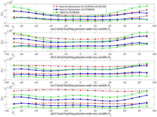
Figure 15.
The lower and the upper bounds under neutral possibility degree.
From these figures, it should be noted that the deviation of the bounds of the interval optimization for PTMRSM is shaper than the deviations of the bounds of the other two optimization methods.
Table 5, Table 6 and Table 7 express the optimal design solutions under the slight level, the strong level, and the absolute level possibility degree.
Table 5.
Optimal solution under the slight possibility degree.
Table 6.
Optimal solution under the strong possibility degree.
Table 7.
Optimal solution under the absolute possibility degree.
From Table 4, Table 5, Table 6 and Table 7, it is obvious that the center point of the critical buckling pressure becomes smaller with the increment of the possible degree. This phenomenon may be due to the fact that the increasing possibility degree limits the space of the optimal solutions. Among the whole optimal design solutions, it can be seen that the interval optimization for PTMRSM always has the smallest radius of the critical buckling pressure. This implies that the interval optimization for PTMRSM can attain robust and efficient optimal design solutions.
Figure 16, Figure 17 and Figure 18 display the lower and the upper bounds of the critical buckling pressure under the slight level, the strong level, and the absolute level possibility degree. From these whole figures, it is clear that the results of the interval optimization for PTMRSM also have the smallest deviations of the bounds compared to the other two optimization methods. It means that the double-loop interval optimization method with PTMRSM has enough efficiency and robustness in contrast to the same interval optimization method with 3rd-order RSM with MLSM and the NINP optimization method.
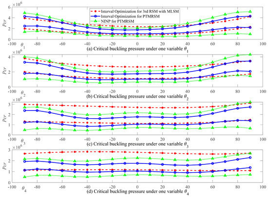
Figure 16.
The lower and the upper bounds under slight possibility degree.
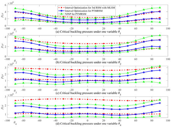
Figure 17.
The lower and the upper bounds under strong possibility degree.
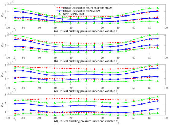
Figure 18.
The lower and the upper bounds under absolute possibility degree.
6. Conclusions
In this paper, a progressive trigonometric mixed response surface method (PTMRSM) was introduced to increase the accuracy of approximation for some high nonlinear engineering problems. The results of two numerical examples and a composite submersible hull were utilized to verify the efficiency and accuracy. For these highly nonlinear complex problems, the PTMRSM may have a better fitting performance and avoid the previous determination of the highest order number of polynomial terms.
Then, the PTMRSM is utilized as one approximate step of the novel double-loop interval optimization method. With the help of the PTMRSM and the amended reliable constraints, the novel double-loop interval optimization process can be constructed, and a composite submersible hull is also performed to verify this new interval optimization method compared with the NINP method and other traditional RSM with the MLSM model. From the comparison results of the composite submersible hull, it can be seen that the double-loop interval optimization for PTMRSM can obtain a robust and efficient optimal design solution.
Furthermore, the center point of the critical buckling pressure becomes smaller with the increase in the possibility degree. This phenomenon may be due to the fact that the increasing possibility degree limits the space of the optimal solutions.
Among the whole optimal design solutions, it can be seen that the interval optimization for PTMRSM always has the smallest radius and deviations of the critical buckling pressure. This implies the double-loop interval optimization for PTMRSM can attain a robust and efficient optimal design solution.
Author Contributions
Conceptualization, G.Z. and W.X.; methodology, G.Z.; software, G.Z.; validation, W.X., M.K.A.B.M.A., N.B.A.A. and S.A.B.A.; writing—original draft preparation, G.Z.; writing—review and editing, M.K.A.B.M.A., N.B.A.A. and S.A.B.A.; supervision, M.K.A.B.M.A. All authors have read and agreed to the published version of the manuscript.
Funding
This paper did not receive any specific grant from funding agencies in the public, commercial, or not-for-profit sectors.
Institutional Review Board Statement
Not applicable.
Informed Consent Statement
Not applicable.
Data Availability Statement
Not applicable.
Acknowledgments
The authors wish to thank Soren Ebbesen for sharing the particle swarm optimization code.
Conflicts of Interest
The authors declare that they have no known competing financial interest or personal relationship that could have appeared to influence the work reported in this paper.
References
- Wu, J.; Zhang, Y.; Chen, L.; Luo, Z. A Chebyshev Interval Method for Nonlinear Dynamic Systems under Uncertainty. Appl. Math. Model. 2013, 37, 4578–4591. [Google Scholar] [CrossRef]
- Wu, J.; Luo, Z.; Zhang, N.; Zhang, Y. A New Interval Uncertain Optimization Method for Structures Using Chebyshev Surrogate Models. Comput. Struct. 2015, 146, 185–196. [Google Scholar] [CrossRef]
- Li, F.; Luo, Z.; Sun, G.; Zhang, N. An Uncertain Multidisciplinary Design Optimization Method Using Interval Convex Models. Eng. Optim. 2013, 45, 697–718. [Google Scholar] [CrossRef]
- Chen, S.H.; Wu, J. Interval Optimization of Dynamic Response for Uncertain Structures with Natural Frequency Constraints. Eng. Struct. 2004, 26, 221–232. [Google Scholar] [CrossRef]
- Qiu, Z.; Elishakoff, I. Anti-Optimization Technique—A Generalization of Interval Analysis for Nonprobabilistic Treatment of Uncertainty. Chaos Solitons Fractals 2001, 12, 1747–1759. [Google Scholar] [CrossRef]
- Moore, R.E.; Kearfott, R.B.; Cloud, M.J. Introduction to Interval Analysis; SIAM: Philadelphia, PA, USA, 2009; Volume 110, ISBN 089871771X. [Google Scholar]
- Elishakoff, I.; Haftka, R.T.; Fang, J. Structural Design under Bounded Uncertainty—Optimization with Anti-Optimization. Comput. Struct. 1994, 53, 1401–1405. [Google Scholar] [CrossRef]
- Ben-Haim, Y. Convex Models of Uncertainty: Applications and Implications. Erkenntnis 1994, 41, 139–156. [Google Scholar] [CrossRef]
- Qiu, Z.; Elishakoff, I. Antioptimization of Structures with Large Uncertain-but-Non-Random Parameters via Interval Analysis. Comput. Methods Appl. Mech. Eng. 1998, 152, 361–372. [Google Scholar] [CrossRef]
- Jiang, C.; Han, X.; Liu, G.R.; Liu, G.P. A Nonlinear Interval Number Programming Method for Uncertain Optimization Problems. Eur. J. Oper. Res. 2008, 188, 1–13. [Google Scholar] [CrossRef]
- Jiang, C.; Han, X.; Guan, F.J.; Li, Y.H. An Uncertain Structural Optimization Method Based on Nonlinear Interval Number Programming and Interval Analysis Method. Eng. Struct. 2007, 29, 3168–3177. [Google Scholar] [CrossRef]
- Jiang, C.; Zhang, Z.G.; Zhang, Q.F.; Han, X.; Xie, H.C.; Liu, J. A New Nonlinear Interval Programming Method for Uncertain Problems with Dependent Interval Variables. Eur. J. Oper. Res. 2014, 238, 245–253. [Google Scholar] [CrossRef]
- Li, F.; Luo, Z.; Rong, J.; Zhang, N. Interval Multi-Objective Optimisation of Structures Using Adaptive Kriging Approximations. Comput. Struct. 2013, 119, 68–84. [Google Scholar] [CrossRef]
- Zhao, Z.; Han, X.; Jiang, C.; Zhou, X. A Nonlinear Interval-Based Optimization Method with Local-Densifying Approximation Technique. Struct. Multidiscip. Optim. 2010, 42, 559–573. [Google Scholar] [CrossRef]
- Cheng, J.; Duan, G.F.; Liu, Z.Y.; Li, X.G.; Feng, Y.X.; Chen, X.H. Interval Multiobjective Optimization of Structures Based on Radial Basis Function, Interval Analysis, and NSGA-II. J. Zhejiang Univ. Sci. A 2014, 15, 774–788. [Google Scholar] [CrossRef]
- Wu, J.; Luo, Z.; Zhang, Y.; Zhang, N.; Chen, L. Interval Uncertain Method for Multibody Mechanical Systems Using Chebyshev Inclusion Functions. Int. J. Numer. Methods Eng. 2013, 95, 608–630. [Google Scholar] [CrossRef]
- Cheng, J.; Liu, Z.; Wu, Z.; Tang, M.; Tan, J. Direct Optimization of Uncertain Structures Based on Degree of Interval Constraint Violation. Comput. Struct. 2016, 164, 83–94. [Google Scholar] [CrossRef]
- Xia, H.; Wang, L.; Liu, Y. Uncertainty-Oriented Topology Optimization of Interval Parametric Structures with Local Stress and Displacement Reliability Constraints. Comput. Methods Appl. Mech. Eng. 2020, 358, 112644. [Google Scholar] [CrossRef]
- Song, X.; Lv, L.; Sun, W.; Zhang, J. A Radial Basis Function-Based Multi-Fidelity Surrogate Model: Exploring Correlation between High-Fidelity and Low-Fidelity Models. Struct. Multidiscip. Optim. 2019, 60, 965–981. [Google Scholar] [CrossRef]
- Parnianifard, A.; Azfanizam, A.S.; Ariffin, M.K.A.; Ismail, M.I.S. Crossing Weighted Uncertainty Scenarios Assisted Distribution-Free Metamodel-Based Robust Simulation Optimization. Eng. Comput. 2020, 36, 139–150. [Google Scholar] [CrossRef]
- Basudhar, A.; Missoum, S. Adaptive Explicit Decision Functions for Probabilistic Design and Optimization Using Support Vector Machines. Comput. Struct. 2008, 86, 1904–1917. [Google Scholar] [CrossRef]
- Havinga, J.; van den Boogaard, A.H.; Klaseboer, G. Sequential Improvement for Robust Optimization Using an Uncertainty Measure for Radial Basis Functions. Struct. Multidiscip. Optim. 2017, 55, 1345–1363. [Google Scholar] [CrossRef]
- Cheng, J.; Liu, Z.; Wu, Z.; Li, X.; Tan, J. Robust Optimization of Structural Dynamic Characteristics Based on Adaptive Kriging Model and CNSGA. Struct. Multidiscip. Optim. 2015, 51, 423–437. [Google Scholar] [CrossRef]
- Wang, G.G. Adaptive Response Surface Method Using Inherited Latin Hypercube Design Points. J. Mech. Des. Trans. ASME 2003, 125, 210–220. [Google Scholar] [CrossRef]
- Chakraborty, S.; Sen, A. Adaptive Response Surface Based Efficient Finite Element Model Updating. Finite Elem. Anal. Des. 2014, 80, 33–40. [Google Scholar] [CrossRef]
- Xu, S.; Feng, N.; Liu, K.; Liang, Y.; Liu, X. A Weighted Fuzzy Process Neural Network Model and Its Application in Mixed-Process Signal Classification. Expert Syst. Appl. 2021, 172, 114642. [Google Scholar] [CrossRef]
- Kim, C.; Wang, S.; Choi, K.K. Efficient Response Surface Modeling by Using Moving Least-Squares Method and Sensitivity. AIAA J. 2005, 43, 2404–2411. [Google Scholar] [CrossRef]
- Youn, B.D.; Choi, K.K. A New Response Surface Methodology for Reliability-Based Design Optimization. Comput. Struct. 2004, 82, 241–256. [Google Scholar] [CrossRef]
- Kaymaz, I.; McMahon, C.A. A Response Surface Method Based on Weighted Regression for Structural Reliability Analysis. Probabilistic Eng. Mech. 2005, 20, 11–17. [Google Scholar] [CrossRef]
- Taflanidis, A.A.; Cheung, S. Stochastic Sampling Using Moving Least Squares Response Surface Approximations. Probabilistic Eng. Mech. 2012, 28, 216–224. [Google Scholar] [CrossRef]
- Li, J.; Wang, H.; Kim, N.H. Doubly Weighted Moving Least Squares and Its Application to Structural Reliability Analysis. Struct. Multidiscip. Optim. 2012, 46, 69–82. [Google Scholar] [CrossRef]
- Lee, S. Reliability Based Design Optimization Using Response Surface Augmented Moment Method. J. Mech. Sci. Technol. 2019, 33, 1751–1759. [Google Scholar] [CrossRef]
- Zheng, G.; Ariffin, M.K.A.B.M.; Ahmad, S.A.B.; Abdul Aziz, N.B.; Xu, W. Robust Optimization of Composite Cylindrical Shell by A Trigonometric Mixed Response Surface Method. Int. J. Numer. Methods Eng. 2022, 123, 5010–5035. [Google Scholar] [CrossRef]
- Gavin, H.P.; Yau, S.C. High-Order Limit State Functions in the Response Surface Method for Structural Reliability Analysis. Struct. Saf. 2008, 30, 162–179. [Google Scholar] [CrossRef]
- Box, G.E.P.; Hunter, J.S. Multi-Factor Experimental Designs for Exploring Response Surfaces. Ann. Math. Stat. 1957, 28, 195–241. [Google Scholar] [CrossRef]
- Lee, Y.J.; Lin, C.C. Regression of the Response Surface of Laminated Composite Structures. Compos. Struct. 2003, 62, 91–105. [Google Scholar] [CrossRef]
- Lin, C.C.; Lee, Y.J. Stacking Sequence Optimization of Laminated Composite Structures Using Genetic Algorithm with Local Improvement. Compos. Struct. 2004, 63, 339–345. [Google Scholar] [CrossRef]
- Zheng, G.; Ariffin, M.K.A.B.M.; Ahmad, S.A.B.; Aziz, N.B.A.; Xu, W. A Novel Progressive Response Surface Method for High-Order Polynomial Metamodel. J. Phys. Conf. Ser. 2022, 2224, 12045. [Google Scholar] [CrossRef]
- Zheng, G.; Yang, X. Studies of the Resistance Optimization of Underwater Vehicle Based on Multiple-Speed Approximate Model. Proceedings of 2018 2nd International Conference on Functional Materials and Chemical Engineering (ICFMCE 2018), Abu Dhabi, United Arab Emirates, 20–22 November 2018; Volume 272, p. 1029. [Google Scholar]
- Muscolino, G.; Sofi, A. Stochastic Analysis of Structures with Uncertain-but-Bounded Parameters via Improved Interval Analysis. Probabilistic Eng. Mech. 2012, 28, 152–163. [Google Scholar] [CrossRef]
- Wu, J.; Zhang, Y.; Chen, L.; Chen, P.; Qin, G. Uncertain Analysis of Vehicle Handling Using Interval Method. Int. J. Veh. Des. 2011, 56, 81–105. [Google Scholar] [CrossRef]
- Jiang, C.; Han, X.; Liu, G.P. A Sequential Nonlinear Interval Number Programming Method for Uncertain Structures. Comput. Methods Appl. Mech. Eng. 2008, 197, 4250–4265. [Google Scholar] [CrossRef]
- Jiang, C.; Han, X.; Liu, G.R. Optimization of Structures with Uncertain Constraints Based on Convex Model and Satisfaction Degree of Interval. Comput. Methods Appl. Mech. Eng. 2007, 196, 4791–4800. [Google Scholar] [CrossRef]
- Wu, J.; Luo, Z.; Zhang, Y.; Zhang, N. An Interval Uncertain Optimization Method for Vehicle Suspensions Using Chebyshev Metamodels. Appl. Math. Model. 2014, 38, 3706–3723. [Google Scholar] [CrossRef]
- Shin, Y.S.; Grandhi, R.V. A Global Structural Optimization Technique Using an Interval Method. Struct. Multidiscip. Optim. 2001, 22, 351–363. [Google Scholar] [CrossRef]
- Wang, L.; Xiong, C.; Wang, X.; Xu, M.; Li, Y. A Dimension-Wise Method and Its Improvement for Multidisciplinary Interval Uncertainty Analysis. Appl. Math. Model. 2018, 59, 680–695. [Google Scholar] [CrossRef]
- Sevastianov, P. Numerical Methods for Interval and Fuzzy Number Comparison Based on the Probabilistic Approach and Dempster-Shafer Theory. Inf. Sci. 2007, 177, 4645–4661. [Google Scholar] [CrossRef]
- Victoire, T.A.A.; Jeyakumar, A.E. Hybrid PSO-SQP for Economic Dispatch with Valve-Point Effect. Electr. Power Syst. Res. 2004, 71, 51–59. [Google Scholar] [CrossRef]
- Zhou, J.; Cheng, S.; Li, M. Sequential Quadratic Programming for Robust Optimization with Interval Uncertainty. J. Mech. Des. 2012, 134, 100913. [Google Scholar] [CrossRef]
- Javidrad, F.; Nazari, M.; Javidrad, H.R. Optimum Stacking Sequence Design of Laminates Using a Hybrid PSO-SA Method. Compos. Struct. 2018, 185, 607–618. [Google Scholar] [CrossRef]


Disclaimer/Publisher’s Note: The statements, opinions and data contained in all publications are solely those of the individual author(s) and contributor(s) and not of MDPI and/or the editor(s). MDPI and/or the editor(s) disclaim responsibility for any injury to people or property resulting from any ideas, methods, instructions or products referred to in the content. |
© 2023 by the authors. Licensee MDPI, Basel, Switzerland. This article is an open access article distributed under the terms and conditions of the Creative Commons Attribution (CC BY) license (https://creativecommons.org/licenses/by/4.0/).