Improved Bathymetry in the South China Sea from Multisource Gravity Field Elements Using Fully Connected Neural Network

Abstract

Traditional bathymetry inversion methods that rely on an altimetry-derived gravity anomaly (GA) and/or a vertical gravity gradient anomaly (VGG) have been widely used for bathymetry prediction in the South China Sea. However, few studies attempt new methods to combine multisource gravity data to improve the accuracy of the bathymetry. In this study, we introduce a fully connected deep neural network (FC-DNN) to merge GA, VGG, and the deflection of vertical (DOV) to predict the bathymetry in the South China Sea. Single beam sounding depths were used as sample data for neural network training. Independent shipboard depths and GEBCO2023, topo_25.1, and ETOPO2022 models were applied as validation data. The assessment results showed that the FC-DNN model reached a high precision level with an STD of 49.20 m. More than 70% of the differences between the FC-DNN bathymetric model and other depth models were less than 100 m. Furthermore, the spectral analysis results showed that the FC-DNN bathymetry model has stronger energy in medium and short wavelengths than other models, which indicates that additional gravity field element DOVs can recover richer topographic signals in those particular bands.

1. Introduction

Bathymetry is an indispensable element of global topography, encompassing an array of geomorphological characteristics, including sea mountains, hills, ridges, submarine trenches, deep ocean basins, and so on. High-resolution, high-accuracy bathymetry is critical for understanding seafloor tectonic movements and seafloor evolutionary processes and for perceiving the influence of bathymetry on ocean circulation, ocean mixing, and climate. It serves as a vital source of data for research in the fields of oceanography, marine geology, marine geophysics, and marine biology. Various technical approaches have been developed over the years to obtain bathymetry data, such as shipboard sonar sounding, laser radar sounding, satellite altimetry gravity data, and remote sensing image inversion. For global bathymetry acquisition, the altimetry-derived gravity field plays an important role in ensuring fast global coverage [1,2].

Even though most marine gravity field elements, including the geoid, the deflection of the vertical (DOV), the gravity anomaly (GA), and the vertical gravity gradient anomaly (VGG), can reflect topographic information to varying degrees, GA is the primary altimetry-derived gravity field element employed in bathymetry inversion, mainly owing to the high correlation between GA and bathymetry over a band of wavelengths. Pioneering studies conducted into the expression of the gravity potential perturbation in the frequency domain [3], the flexural isostatic compensation theory [4], and the bathymetry prediction from Seasat satellite altimeter gravity profiles [5] have analyzed the correlation between gravity data and bathymetry, demonstrating the feasibility of predicting bathymetry from altimetry-derived gravity data. Smith and Sandwell (1994) [6] further advanced an admittance theory and calculated the bathymetry in the Southern Oceans by integrating dense gravity anomalies and sparse shipboard sounding data. The admittance method in the frequency domain has been widely verified and has emerged as one of the primary methods for bathymetry prediction [7,8,9,10,11,12,13]. In the spatial domain, the gravity geological method (GGM) has been proposed and commonly used for bathymetry inversion in the South China Sea, Drake Passage, southern Greenland, southern Alaska, and other territories [14,15,16,17]. GGM is known to be effective in improving the accuracy of bathymetry, particularly in sea areas with rich shipboard sounding data. Nevertheless, there is still a gap between the accuracy of the predicted bathymetry and the multibeam sounding depths, so that the predicted model cannot accurately reflect the minute features of the seafloor.

Research on combining more gravity data and optimizing algorithms has been conducted by many scholars to further improve the accuracy of the bathymetry model. As it can reflect more short-wavelength topographic information, VGG has been employed to predict bathymetry when combined with GA. The primary focus of these studies has been centered around the correlation between VGG and bathymetry and how they can be jointly used to construct bathymetry with GA. Wang (2000) [18] presented a least-squares method for bathymetry prediction using VGG, which confirmed its feasibility. Fan et al. (2020) [19] proposed a nonlinear iterative least-squares method for bathymetry estimation by merging GA and VGG in the space domain. Hu et al. (2014, 2021) [20,21] used GA, VGG, and shipborne depths to construct a global bathymetry model, and the results proved that combining GA and VGG can improve the accuracy of bathymetry. However, the fusion inversion required a specific relationship between the gravity data and the bathymetry in different wavelength ranges, and the extraction of components can make the fusion process complicated. If additional gravity field elements (such as DOV) are added, the fusion process becomes more difficult to implement. Like the GA and VGG, the DOV has been demonstrated to be suitable for bathymetry inversion [22,23].

Neural networks, with their powerful massive data processing and nonlinear mapping capabilities, have emerged as an ideal tool in the field of earth science. Perol et al. (2018) [24] presented a convolutional neural network for earthquake detection and location from a single waveform. Wu et al. (2022) [25] applied a back propagation neural network to recover ocean significant wave heights from S1 SAR data. Sun et al. (2022) [26] and Annan and Wan (2022) [23] introduced neural networks into the bathymetric prediction field for merging gravity field elements and improved the accuracy of bathymetry in the Gulf of Guinea and Mariana Trench regions. These studies show that neural networks have the potential to contribute a technical approach for bathymetry inversion by combining multi-source gravity field elements. The fully connected deep neural network is the basic type of network in deep learning, where each neuron is connected to all the neurons in the previous and subsequent layers. It can learn complex features of input data and perform tasks such as classification and regression. Fully connected deep neural networks have powerful nonlinear fitting capabilities and can fit most functions. Bathymetry inversion from a marine gravity field is a typical nonlinear problem. Therefore, a fully connected neural network may have strong potential in the field of bathymetry inversion.

In this paper, we selected the South China Sea as the study area, used multi-source altimetry-derived gravity field elements GA, VGG, and DOV as our input data, and high-precision shipboard depths as our training and verification data. To improve the accuracy of predicted bathymetry in this region, we designed a fully connected back propagation deep neural network (FC-DNN). Finally, we evaluated the accuracy and effectiveness of neural network methodology by comparing it with the GEBCO2023, ETOPO2022, and topo_25.1 datasets, as well as shipboard depths.

2. Study Area and Data

2.1. Study Area

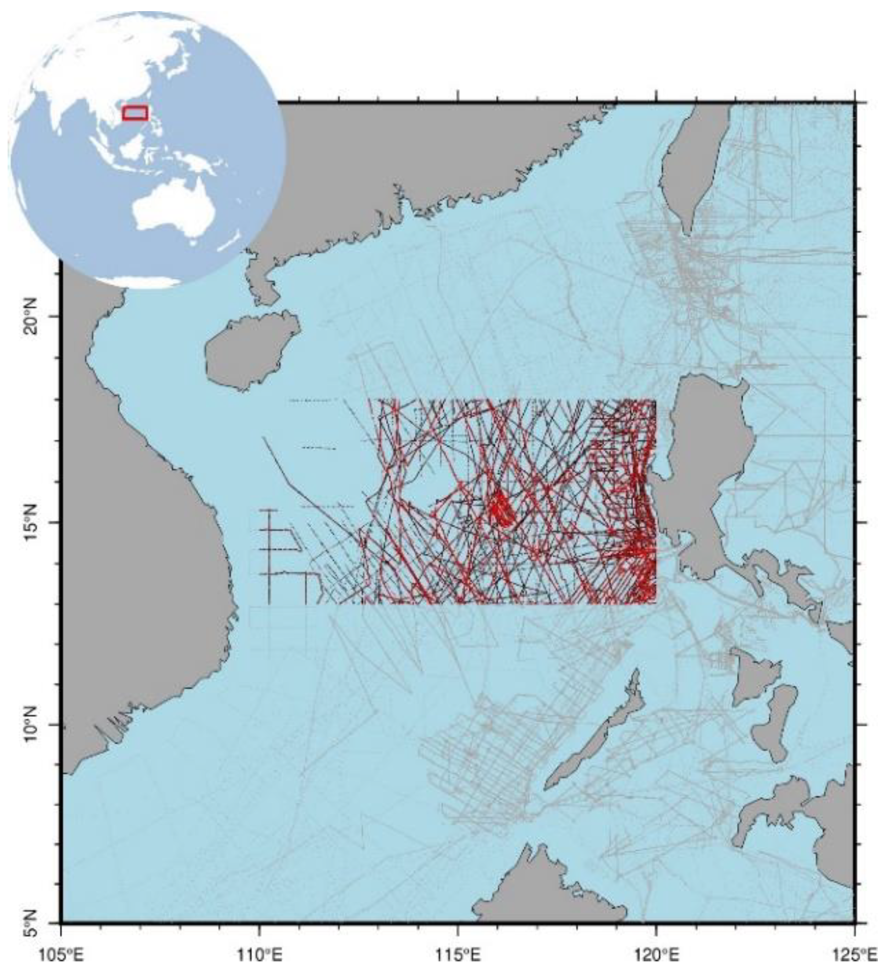
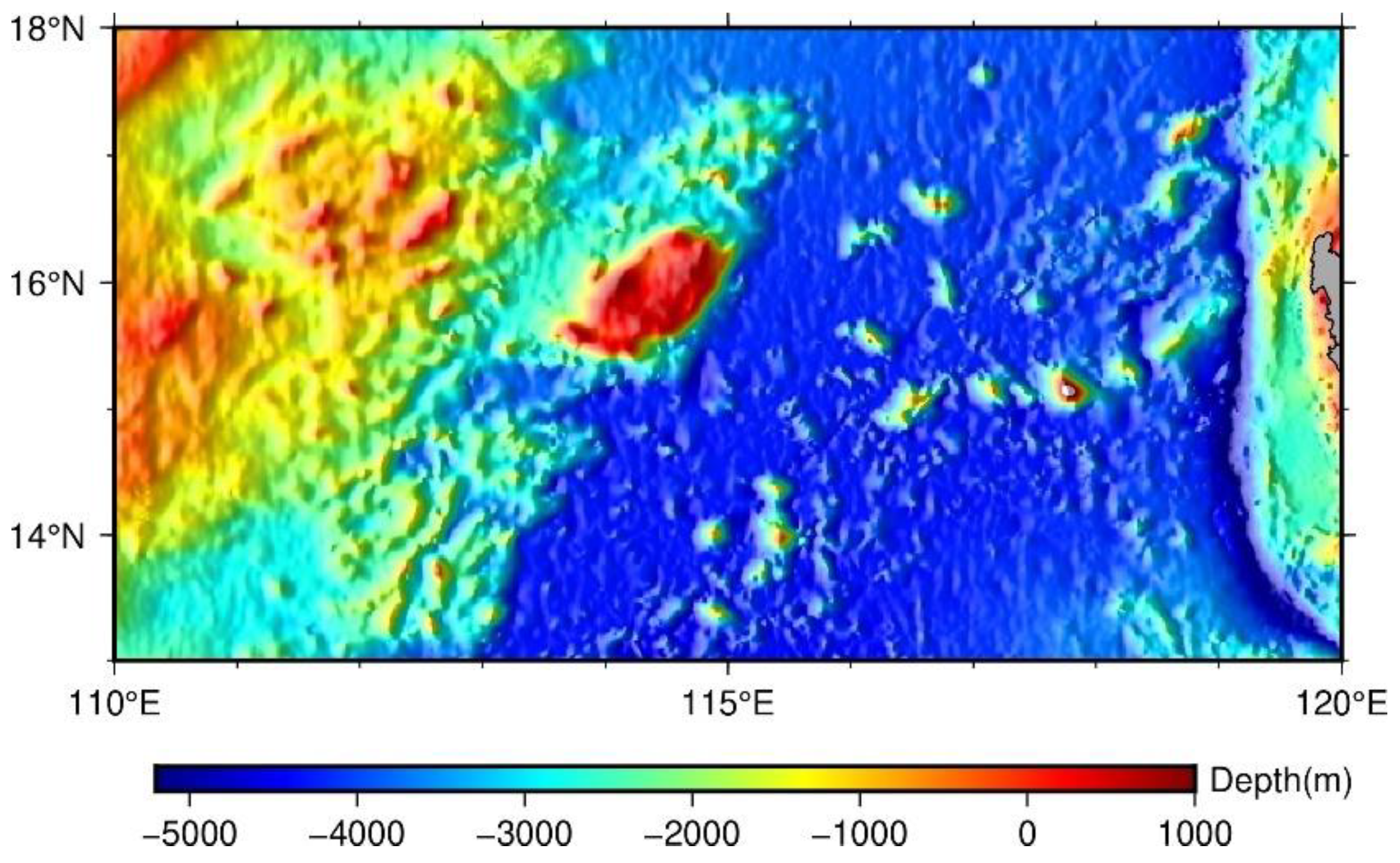
The study area was in the South China Sea, with geographic coordinates of 110° E–120° E and 13° N–18° N (Figure 1). The topography of this region is quite undulating, with depths ranging from −5000 m to 0. The landforms in this region are complex and diverse, including seamounts, sea basins, and trenches, among others, which can be used to verify the performance of the fully connected neural network method for bathymetry inversion.

2.2. Datasets Used

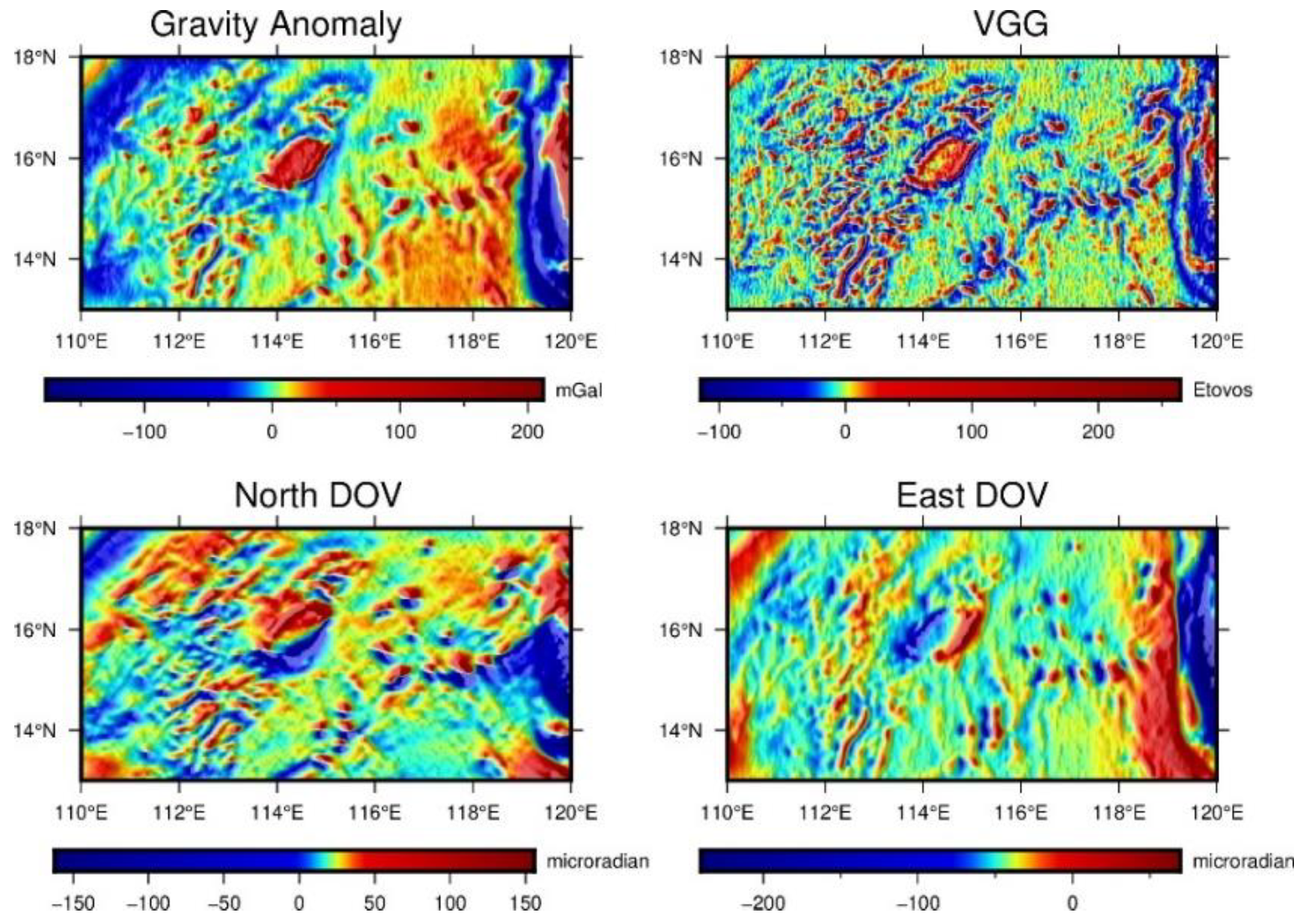
The altimetry-derived gravity field elements used in this study, including DOVs, GA, and VGG data, are the latest version V32.1 with spatial resolution 1’ × 1’ from the Scripps Institution of Oceanography (SIO; the website is https://topex.ucsd.edu/pub/, accessed on 1 February 2023) (Figure 2). The gravity field was taken from the Jason-1/2, SARAL/Altika, Cryosat-2, and Sentinel-3A/B data, and waveform retracking was performed to improve the accuracy of the sea surface heights in the coastal area. As shown in Figure 1 and Figure 2, the GA and VGG have strong correlations with the bathymetry, but the DOVs are weakly correlated with the bathymetry. Even so, the DOVs can also reflect topographic information in regions with rugged topography, such as seamounts and trenches. The accuracy of the altimetry-derived gravity field model has reached a high level, with 1–2 mGal in some deep ocean regions, which shows potential for improving the accuracy of bathymetry [27,28].

The shipborne depth data used in this study were the single-beam sounding data from the National Centers for Environmental Information (NCEI). The total number of shipborne depth points is 112,664, and the distribution is shown in Figure 3. To ensure the quality of shipborne depths, we employed the GEBCO_2023 as an a priori model for outlier detection. We computed the differences between the GEBCO_2023 and the shipborne depths at shipborne sounding points and eliminated shipborne depths with differences greater than 500 m. After quality control, 106,207 sounding points had been obtained, and the data elimination rate was approximately 5.7%. About 20% (21,243, red dots in Figure 3) of the points were picked evenly as check points, and the remaining data (black dots in Figure 3) were selected as control points to compute the bathymetry model.

To validate the accuracy of the predicted bathymetry model, we compared it with existing and widely used models, including GEBCO_2023, topo_25.1, and ETOPO2022. The GEBCO_2023 grid is a comprehensive global terrain model encompassing both ocean and land, with a spatial resolution of 15 arc seconds. It builds upon the SRTM15+ data set version 2.5.5, covering latitudes ranging from 50° South to 60° North [11]. This data set is a fusion of land topography with measured and estimated seafloor topography. It uses predicted ocean depths derived from the V32 gravity model [28]. A large amount of multibeam data and ‘remove-restore’ blending procedure are used to augment the data set, ensuring a continuous, high-resolution bathymetry grid. The Topo_25.1 model, released by SIO in 2023, is a global terrain model for the ocean, mainly covering between 80° S and 80° N, with a spatial resolution of 1 min. The ETOPO2022 is a release of NOAA’s (National Oceanic and Atmospheric Administration) ‘Earth Topography’ dataset. It is a full-coverage, seamless, gridded topographic and bathymetric elevation dataset. It blends a large amount of elevation data from different institutions, including GEBCO2022, shallow bathymetry everywhere, BlueTopo, NOAA Regional DEMs, and others, culminating in a spatial resolution of 15 arc seconds [29].

3. Methodology

3.1. Gravity Field Processing

As is well known, the relationship between the GA and bathymetry data is nonlinear [3], particularly showcasing a strong correlation within the medium- and short-wavelength bands [6]. To address this nonlinear problem, the ‘remove-restore’ technique, which involves linearizing the problem by using a suitable reference field, was employed in this study. The fundamental principle is to decompose the field into a long-wavelength component, which serves as the reference field, and a short-wavelength component, which serves as the residual field [30]. In this study, the GA field was decomposed into a long-wavelength component and a short-wavelength component. The short-wavelength GA exhibited a significant correlation with the bathymetry data and was thus combined with the VGG and north and east components of DOV to predict bathymetry. Referring to GGM [14], the expression for the short-wavelength GA can be formulated as follows:

$$\Delta g_{short}=2\pi G\Delta \rho \left(E-D\right)$$

(1)

where Δg_short is the short-wavelength GA, Δρ is the density difference between seawater and lithosphere, E is shipboard depths at control points, and D is the reference depth, generally taken to be the deepest value of all shipboard depths.

The short-wavelength GA at the control points can be calculated by the Formula (1) for neural network training. It is necessary to calculate the short-wavelength GA of the entire study area for bathymetry inversion. Considering the smooth distribution of the long-wavelength signal and the limited error introduced by interpolation processing, we first subtracted the short-wavelength GA data from the GA data to derive the long-wavelength GA data at the control points. Then, the long-wavelength GA grid of the entire study area was obtained by interpolation. Finally, by subtracting the long-wavelength GA data from the GA data, we obtained the short-wavelength GA grid of the entire study area.

3.2. Bathymetry Inversion Process

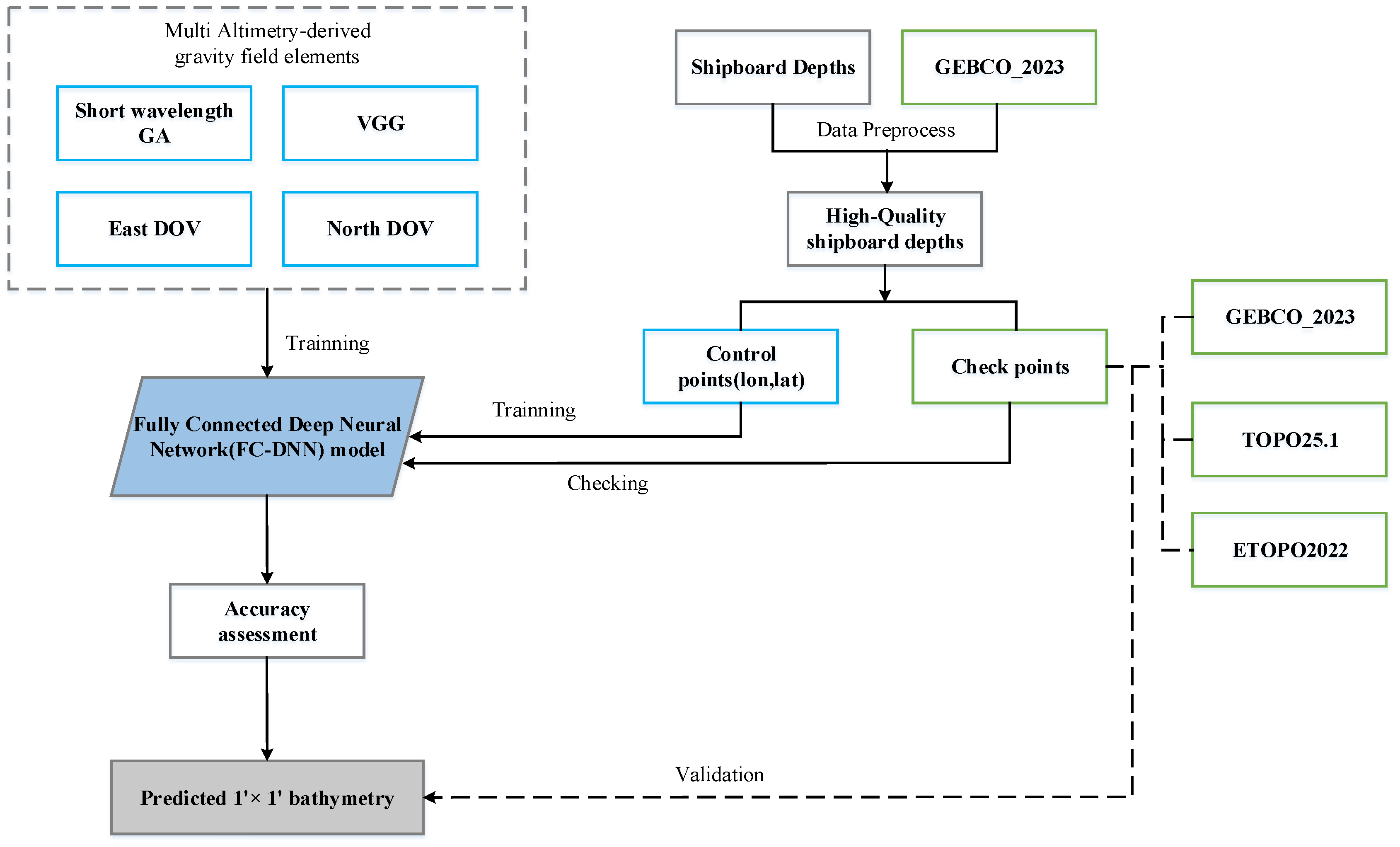
The data processing procedure proposed in this study is shown in Figure 4. Four input altimetry-derived gravity elements were used to compute the bathymetry model, namely: short-wavelength GA, VGG, east component of DOV, and the north component of DOV. High-precision shipboard depths played an important role in training and validating the FC-DNN model. First, after quality control, high-quality shipboard depths were divided into control points and check points. The longitudes, latitudes, GAs, VGGs, east DOVs, and north DOVs on the control points were treated as samples, and the fully connected neural network was trained iteratively with the check data, resulting in a well-trained neural network model. The four altimetry-derived gravity elements in the whole study area were fed into the well-trained FC-DNN model to predict the bathymetry model. Then, the predicted bathymetry model was compared with the shipboard depth checking data and exiting bathymetry models GEBCO_2023, topo_25.1, and ETOPO2022 for accuracy validation.

3.3. Neural Network Structure

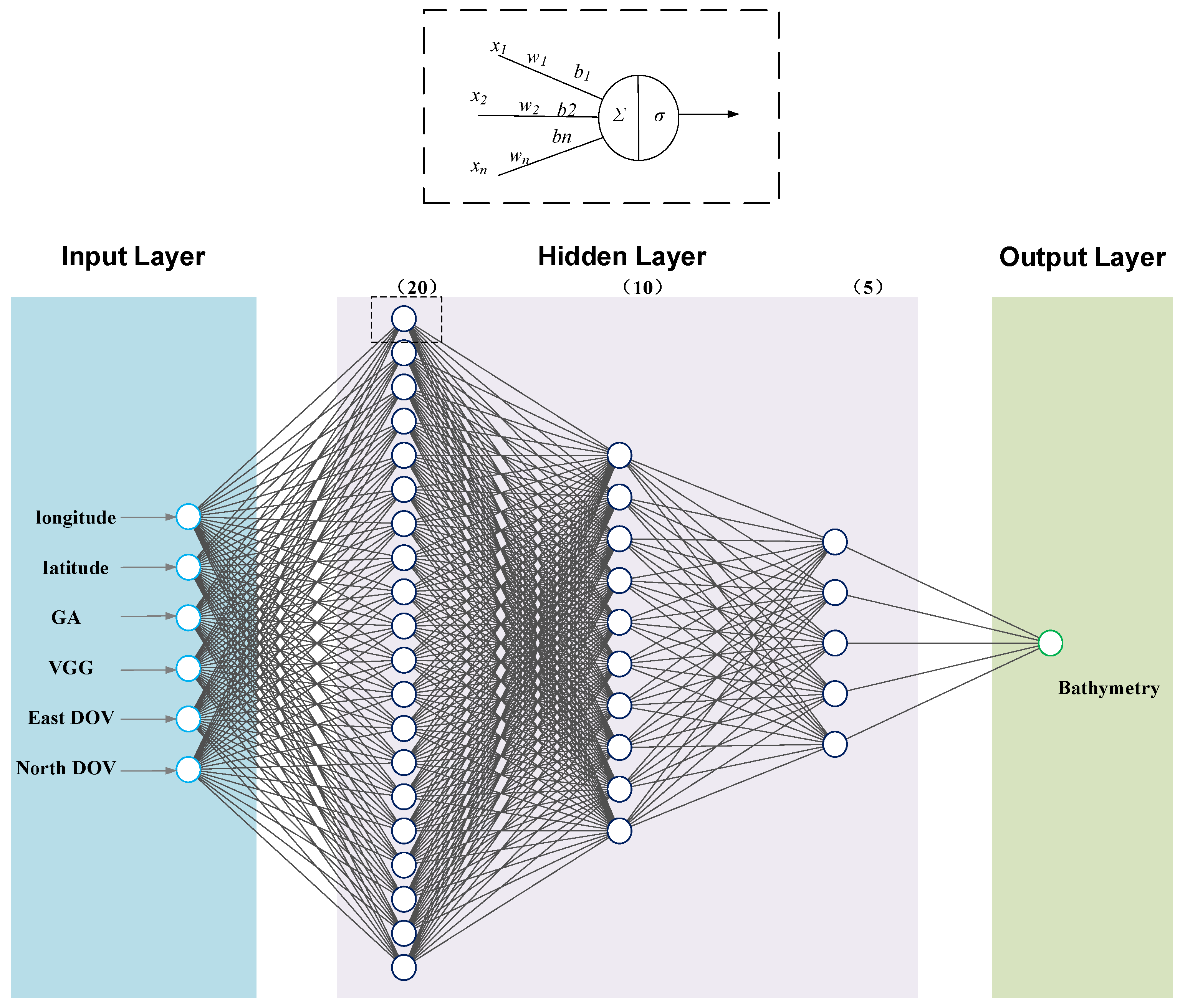
In this study, a fully connected deep neural network (FC-DNN) model was constructed to predict bathymetry using GA, VGG, East DOV, and North DOV. It contained one input layer, multiple hidden layers, and one output layer, as shown in Figure 5. The positions of the gravity field also have an impact on bathymetry; hence, the input layer contained the longitudes and latitudes of the gravity field, except for GA, VGG, East DOV, and North DOV. Hidden layers are helpful when extracting data features, but excessive hidden layers may lead to prolonged training time and overfitting. To achieve an optimal balance, our FC-DNN model was composed of three hidden layers, with 20 neurons in the first layer, 10 neurons in the second layer, and 5 neurons in the third layer after many experiments. Finally, the output layer obtained the bathymetry model after calculation.

Each neuron in the FC-DNN model uses specific operations to extract data features. The neurons in each layer are connected to each other by weight and bias, as shown in the upper dotted box in Figure 5. This process can be expressed as follows:

$$y=\sigma \left(\Sigma \right)=\sigma \left({\displaystyle \sum _{i=1}^n\left(w_i{x}_i+b_i\right)}\right)$$

(2)

where x_i represent the input gravity field signals, y represents the output of the neuron, w_i and b_i denote the weight of each input and bias of the neuron, respectively, and σ represents the activation function, which makes the neuron generate nonlinear outputs. In this study, the rectified Linear Units (ReLU) activation function was used.

Note that, prior to the activation function, it is necessary to normalize the datasets to ensure they fall within the range of 0 to 1. This normalization process is crucial for network convergence and can address the issue of the ReLU activation function setting negative values of the location information and gravity field signals and all output depths to zero [22].

The FC-DNN also contains backward propagation processes to optimize the network. These processes primarily serve to adjust the weights of the neural network. The neural network weights and biases are assigned initial values during the network initialization phase. During training, the weights of each neuron are then adjusted based on predicted differences, which allows for iterative refinement of the network’s performance.

$$w^{\prime }=w-\alpha \frac{\partial loss}{\partial w}$$

(3)

where w′ represents the adjusted weight, α denotes the learning rate, loss represents the loss function which depends on the mean square error. During training, the neural network carries out a backward computation for each forward computation. Finally, the weights are adjusted to attain optimal values that minimize the differences between the predicted bathymetry and the shipborne depths.

3.4. Training the Network and Prediction

After constructing the neural network structure, it is necessary to use the sample data to train the neural network. High-quality shipboard depths at control points were employed as training data, while the remaining check data were used for testing. The neural network was trained as follows.

Firstly, the training and gravity field element data were normalized simultaneously by maximum and minimum standardization to map all data between 0 and 1. This minimized the differences between the input variables.

Secondly, the neural network model was initialized, and the initial weights and biases were generated randomly.

Thirdly, the network was trained for 30 epochs with an initial learning rate of 0.001, using a loss function based on the root mean squared error between predicted and shipborne depths. The value of epochs represents the number of times that the entire training data is fed to the neural network for training. Following epoch 14, the learning rate decreased to 0.000125. To update the weights according to the learning rate and the loss function, the Adam optimization algorithm was utilized. The diverse parameters of the neural network were adjusted to optimize performance.

Finally, by feeding the altimetry-derived gravity signals to the well-trained neural network, the predicted bathymetry in study area was obtained.

4. Results and Evaluation

4.1. FC-DNN-Derived Bathymetry

The bathymetry model in the study area was derived from multi-source gravity field elements. The FC-DNN is presented in Figure 6. As is shown in Figure 6, the depth of the predicted bathymetry model ranges from −5200 m to 0 m, which can accurately reflect the geomorphic features of the study area and clearly reveal geomorphic details such as seamounts, trenches, and submarine basins. The spatial distribution of the bathymetry was highly consistent with that of GEBCO and other bathymetric models, with only minor differences in some details.

4.2. Compared with Shipboard Depths

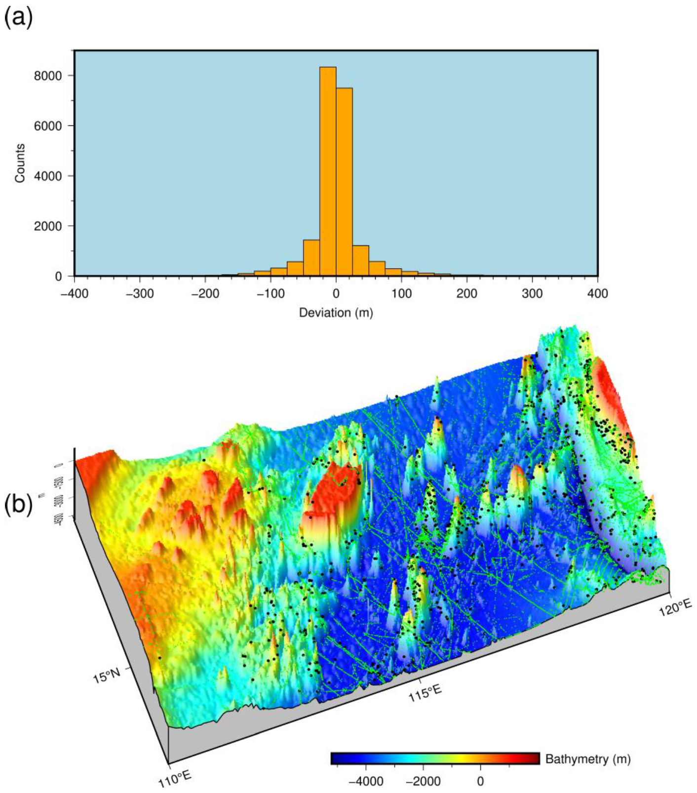
To evaluate the accuracy of the predicted bathymetric model, we compared it with the check points of shipboard depths that were excluded from the neural network training. The deviations of the predicted model from the shipboard depths were calculated, and the results showed that 95.29% of the deviations were less than 100 m, with only a few points having relatively large deviations (as shown in Figure 7a). The spatial distribution of the deviations is presented in Figure 7b; the black dots denote points with absolute deviations greater than 100 m, and the green dots denote those with absolute deviations less than 100 m. Figure 7b shows that the large deviations of the predicted bathymetric model from the shipboard depths are principally distributed in the eastern and central regions where features such as trenches and seamounts exist and the topography changes rapidly. The reason may be that in the east, due to the influence of land, the accuracy of the altimetry-derived marine gravity field is relatively low, thus limiting the accuracy of bathymetry inversion. In addition, in regions with dramatic relief, the accuracy of shipboard depths will also be affected to a certain extent.

Furthermore, we analyzed the differences between the FC-DNN-predicted bathymetry model and the shipboard check points, as well as the correlation coefficient, which is shown in

Table 1. The statistics of the differences between bathymetric models and shipboard depths.

	Max (m)	Min (m)	Mean (m)	STD (m)	Correlation Coeff. (%)
FC-DNN model	860.02	−983.36	0.48	49.20	99.87
GEBCO2023	1853.50	−2316.18	8.36	90.59	99.54
topo_25.1	712.84	−605.16	2.33	83.10	99.61
ETOPO2022	1171.14	−1727.00	−4.63	89.80	99.55

. To assess the accuracy effectively, the statistics of the differences and correlation coefficients between the GEBCO2023, topo_25.1, and ETOPO2022 models and the shipboard depths at check points were also calculated. The STD of the differences between the FC-DNN bathymetric model and check points was 49.20 m, which was a large improvement compared to those of the GEBCO2023, topo_25.1, and ETOPO2022 models. The correlation coefficient between the FC-DNN bathymetry model and the shipboard depths was 99.87%, which was slightly higher than the other models. These results show that the FC-DNN method for bathymetry inversion is feasible and that the inversion results can achieve high accuracy.

4.3. Compared with Promising Bathymetry Models

To further evaluate the accuracy of the FC-DNN model, we compared it to the GEBCO2023, topo_25.1, and ETOPO2022 models directly. The differences between the FC-DNN model and other models were calculated and are shown in Figure 8. Figure 8a–c shows the spatial distribution of differences between the FC-DNN model and GEBCO2023, topo_25.1, and ETOPO2022 models, respectively. In addition, the proportions of the differences in different value ranges were calculated. Figure 8d shows a histogram distribution of the differences between the FC-DNN model and other models. Among them, the blue bar represents the distribution of differences between the FC-DNN model and the GEBCO2023 model, the orange bar denotes those between the FC-DNN model and the topo_25.1 model, and the gray bar denotes those between the FC-DNN model and the ETOPO2022 model.

In general, Figure 8 shows that the FC-DNN-predicted bathymetry model agrees well with the GEBCO2023, topo_25.1, and ETOPO2022 models, except for large differences in some areas. To be specific, Figure 8a–c show that there are large differences between the FC-DNN model and the GEBCO2023, topo_25.1, and ETOPO2022 models in the northwest region of the study area (regions in dashed lines), but small differences in the central and eastern regions. The differences for GEBCO2023, shown in Figure 8a, are more obvious. The reason may be related to the distribution of shipboard depths. Shipboard depths are dense and well-proportioned in the central and eastern regions, as shown in Figure 3. The FC-DNN method uses shipboard depths as the sample data for training the neural network. The accuracy of the FC-DNN-predicted bathymetry model therefore depends to some extent on the distribution of shipboard depths. Hence, in the area with fewer shipboard depths, the accuracy of predicted bathymetry is relatively low, and its deviations from other models are large. Figure 8d shows that about 70% of the deviations between the FC-DNN model and the GEBCO2023, topo_25.1, and ETOPO2022 models are less than 100 m, and over 85% are less than 200 m, illustrating that the FC-DNN model agrees well with other models. Compared to GEBCO2023, the differences for topo_25.1 and ETOPO2022 models are similar, and the proportion of differences less than 100 m is slightly higher, indicating that the FC-DNN model is in better agreement with the topo_25.1 and ETOPO2022 models.

To further analyze the correlation between the FC-DNN model and other models, the statistics of the differences and the correlation coefficients between the FC-DNN model and other models were calculated and are shown in

Table 2. The statistics of the differences between bathymetric models and other models.

	Max (m)	Min (m)	Mean (m)	STD (m)	Correlation Coeff. (%)
FC-DNN model VS GEBCO2023	1878.87	−3561.00	−33.18	184.33	99.01
FC-DNN model VS topo_25.1	1826.79	−2124.25	−8.62	162.09	99.23
FC-DNN model VS ETOPO2022	1801.71	−2470.54	−15.56	167.93	99.17

. Table 2 further confirms that the FC-DNN model is in better agreement with the topo_25.1 and ETOPO2022 models than the GEBCO2023 model, with STDs of 162.09 m and 167.93 m and correlation coefficients of 99.23% and 99.17%, compared with the STD of 184.33 m and correlation coefficient of 99.01% for GEBCO2023. This may be due to the fact that the GEBCO2023 combined more multibeam data and used an applied ‘remove-restore’ blending procedure to augment the dataset, making it more different from other models.

Spectral analysis can decompose signals or data into multiple frequency components and analyze the power distribution characteristics of signals or data at different frequencies. Calculating the power spectral density (PSD) in the radial direction is a common method for spectral analysis. Many scholars have used PSD for bathymetry model assessment since a higher PSD indicates a higher topographic signal at the same wavelength [16,26]. The amplitude of the PSD in the radial direction is calculated as 10log₁₀ (P), where P represents the relevant power expressed in dB. Figure 9 shows the PSD of the bathymetry models in the entire gridded region, where the black line represents the PSD of the FC-DNN-predicted bathymetry model, the red line represents the GEBCO2023 model, the blue line represents the topo_25.1 model, and the green line represents the ETOPO2022 model.

As illustrated in Figure 9, at long wavelengths greater than 100 km, the PSDs of the four bathymetric models are comparable. At medium and short wavelengths, between 20 km and 100 km, the FC-DNN-predicted bathymetric model generated a high PSD, which suggests that the FC-DNN model contains more medium- and short-wavelength topographic details than the GEBCO2023, topo_25.1, and ETOPO2022 models. The reason for this may be that the FC-DNN bathymetry model was derived from additional gravity element DOVs compared to the GEBCO2023, topo_25.1, and ETOPO2022 models, and the DOVs have strong coherence with bathymetry in the 20~100 km band [23]. This shows that DOV can be used as an effective data source for bathymetry inversion and thus improve the accuracy of bathymetry models in the South China Sea. At short wavelengths less than 20 km, the GEBCO2023 model generates a high PSD, but the PSD of the FC-DNN model is relatively lower than those of the other three models. This may be caused by the GEBCO2023 model having been merged with more multibeam sounding data, which contains more short-wavelength topographic details.

5. Conclusions

In this study, a fully connected deep neural network has been applied to predict the bathymetry model in the South China Sea by merging multi-source gravity field elements. To assess the accuracy of the inversed bathymetry model, we compared it to independent shipboard depths and promising high-precision bathymetric models GEBCO2023, topo_25.1, and ETOPO2022, and the differences and correlation coefficients between each of them were calculated. The results showed that the FC-DNN method could predict ocean depths effectively using a simplified fusion of gravity field elements GA, VGG, and DOVs. The predicted model reached a high precision level, with an STD of 49.20 m compared to the shipboard depths, which was much higher than that of the GEBCO2023 model, which had an STD of 90.59 m, the topo_25.1 model, which had an STD of 83.10 m, and the ETOPO2022 model, which had an STD of 89.80 m. More than 70% of the differences between the predicted bathymetry model and other depths were less than 100 m, and about 85% were less than 200 m. The correlation coefficients between the FC-DNN bathymetry model and other depths exceeded 99%, suggesting that the FC-DNN-predicted bathymetry model agrees well with other bathymetric models. In addition, the PSDs of four bathymetry models were also calculated. The results showed that the FC-DNN bathymetry model had more vital energy in the short-to-medium wavelength band of 20–100 m than other models, which indicates that additional gravity field element DOVs can recover more accurate topographic signals in a particular band and can be used as one of the effective data sources for bathymetry inversion.

References

1. Sun, H.; Li, Q.; Bao, L.; Wu, Z.; Wu, L. Progress and Development Trend of Global Refined Seafloor Topography Modeling. Geomat. Inf. Sci. Wuhan Univ. 2022, 47, 1555–1567. (In Chinese) [Google Scholar]
2. Eppelbaum, L.V.; Katz, Y.I. A New Regard on the Tectonic Map of the Arabian-African Region Inferred from the Satellite Gravity Analysis. Acta Geophys. 2017, 65, 607–626. [Google Scholar] [CrossRef]
3. Parker, R. The rapid calculation of potential anomalies. Geophys. J. Int. 1972, 31, 447–455. [Google Scholar] [CrossRef] [Green Version]
4. Watts, A.B. An analysis of isostasy in the world’s oceans 1. Hawaiian-Emperor Seamount Chain. J. Geophys. Res. Solid Earth 1978, 83, 5989–6004. [Google Scholar] [CrossRef] [Green Version]
5. Dixon, T.H.; Naraghi, M.; McNutt, M.K.; Smith, S.M. Bathymetric prediction from SEASAT altimeter data. J. Geophys. Res. Atmos. 1983, 88, 1563–1571. [Google Scholar] [CrossRef]
6. Smith, W.H.F.; Sandwell, D.T. Bathymetric prediction from dense satellite altimetry and sparse shipboard bathymetry. J. Geophys. Res. Solid Earth 1994, 99, 21803–21824. [Google Scholar] [CrossRef]
7. Smith, W.H.F.; Sandwell, D.T. Global Sea Floor Topography from Satellite Altimetry and Ship Depth Soundings. Science 1997, 277, 1956–1962. [Google Scholar] [CrossRef] [Green Version]
8. Amante, C.; Eakins, B.W. ETOPO1 1 Arc-Minute Global Relief Model: Procedures, Data Sources and Analysis. Psychologist 2009, 16, 20–25. [Google Scholar]
9. Becker, J.J.; Sandwell, D.T.; Smith, W.H.F.; Braud, J.; Binder, B.; Depner, J.; Fabre, D.; Factor, J.; Ingalls, S.; Kim, S.-H.; et al. Global Bathymetry and Elevation Data at 30 Arc Seconds Resolution: SRTM30_PLUS. Mar. Geod. 2009, 32, 355–371. [Google Scholar] [CrossRef]
10. Li, Q.; Bao, L. Predicting Submarine Topography of the South China Sea from Altimetry Gravity Field with High Precision. Hydrogr. Surv. Charting 2016, 36, 1–5. (In Chinese) [Google Scholar]
11. Mayer, L.; Jakobsson, M.; Allen, G.; Dorschel, B.; Falconer, R.; Ferrini, V. The Nippon Foundation—GEBCO Seabed 2030 Project: The Quest to See the World’s Oceans Completely Mapped by 2030. Geosciences 2018, 8, 63. [Google Scholar] [CrossRef] [Green Version]
12. Tozer, B.; Sandwell, D.T.; Smith, W.H.F.; Olson, C.; Beale, J.R.; Wessel, P. Global Bathymetry and Topography at 15 Arc Sec: SRTM15+. Earth Space Sci. 2019, 6, 1847–1864. [Google Scholar] [CrossRef]
13. Hu, M.; Jin, T.; Jiang, W.; Chu, Y.; Li, J. Bathymetry Model in the Northwestern Pacific Ocean Predicted from Satellite Altimetric Vertical Gravity Gradient Anomalies and Ship-Board Depths. Mar. Geod. 2021, 45, 24–46. [Google Scholar] [CrossRef]
14. Hsiao, Y.-S.; Kim, J.W.; Kim, K.B.; Lee, B.Y.; Hwang, C. Bathymetry Estimation Using the Gravity-Geologic Method: An Investigation of Density Contrast Predicted by the Downward Continuation Method. Terr. Atmos. Ocean Sci. 2011, 22, 347. [Google Scholar] [CrossRef] [Green Version]
15. Hsiao, Y.-S.; Hwang, C.; Cheng, Y.-S.; Chen, L.-C.; Hsu, H.-J.; Tsai, J.-H. High-resolution depth and coastline over major atolls of South China Sea from satellite altimetry and imagery. Remote Sens. Environ. 2016, 176, 69–83. [Google Scholar] [CrossRef]
16. Kim, K.B.; Hsiao, Y.-S.; Kim, J.W.; Lee, B.Y.; Kwon, Y.K.; Kim, C.H. Bathymetry enhancement by altimetry-derived gravity anomalies in the East Sea (Sea of Japan). Mar. Geophys. Res. 2010, 31, 285–298. [Google Scholar] [CrossRef]
17. Ouyang, M.; Sun, Z.; Zhai, Z. Predicting bathymetry in South China Sea using the gravity-geologic method. Chin. J. Geophys. 2014, 57, 2756–2765. (In Chinese) [Google Scholar]
18. Wang, Y.M. Predicting Bathymetry from the Earth’s Gravity Gradient Anomalies. Mar. Geod. 2000, 23, 251–258. [Google Scholar] [CrossRef]
19. Fan, D.; Li, S.; Li, X.; Yang, J.; Wan, X. Seafloor Topography Estimation from Gravity Anomaly and Vertical Gravity Gradient Using Nonlinear Iterative Least Square Method. Remote Sens. 2020, 13, 64. [Google Scholar] [CrossRef]
20. Hu, M.; Li, J.; Li, H.; Shen, C.; Jin, T.; Xing, L. Predicting Global Seafloor Topography Using Multi-Source Data. Mar. Geod. 2014, 38, 176–189. [Google Scholar] [CrossRef]
21. Hu, M.; Li, L.; Jin, T.; Jiang, W.; Wen, H.; Li, J. A New 1′ × 1′ Global Seafloor Topography Model Predicted from Satellite Altimetric Vertical Gravity Gradient Anomaly and Ship Soundings BAT_VGG2021. Remote Sens. 2021, 13, 3515. [Google Scholar] [CrossRef]
22. Wan, X.; Liu, B.; Sui, X.; Annan, R.F.; Hao, R.; Min, Y. Bathymetry inversion using the deflection of the vertical: A case study in South China Sea. Geod. Geodyn. 2022, 13, 492–502. [Google Scholar] [CrossRef]
23. Annan, R.F.; Wan, X. Recovering Bathymetry of the Gulf of Guinea Using Altimetry-Derived Gravity Field Products Combined via Convolutional Neural Network. Surv. Geophys. 2022, 43, 1541–1561. [Google Scholar] [CrossRef]
24. Perol, T.; Gharbi, M.; Denolle, M. Convolutional Neural Network for Earthquake Detection and Location. Sci. Adv. 2018, 4, e1700578. [Google Scholar] [CrossRef] [PubMed] [Green Version]
25. Wu, K.; Li, X.-M.; Huang, B. Retrieval of Ocean wave heights from spaceborne SAR in the Arctic Ocean with a neural network. J. Geophys. Res. Ocean 2021, 126, e2020JC016946. [Google Scholar] [CrossRef]
26. Sun, H.; Feng, Y.; Fu, Y.; Sun, W.; Peng, C.; Zhou, X. Bathymetric Prediction Using Multisource Gravity Data Derived from a Parallel Linked BP Neural Network. J. Geophys. Res. Solid Earth 2022, 127, e2022JB024428. [Google Scholar] [CrossRef]
27. Sandwell, D.T.; Muller, R.D.; Smith, W.H.; Garcia, E.; Francis, R. Marine geophysics. New global marine gravity model from CryoSat-2 and Jason-1 reveals buried tectonic structure. Science 2014, 346, 65–67. [Google Scholar] [CrossRef]
28. Sandwell, D.; Harper, H.; Tozer, B.; Smith, W. Gravity Field Recovery from Geodetic Altimeter Missions. Adv. Space Res. 2019, 68, 1059–1072. [Google Scholar] [CrossRef]
29. NOAA National Centers for Environmental Information. 2022: ETOPO 2022 15 Arc-Second Global Relief Model; NOAA National Centers for Environmental Information: Asheville, NC, USA, 2022. [Google Scholar] [CrossRef]
30. Hwang, C. A Bathymetric Model for the South China Sea from Satellite Altimetry and Depth Data. Mar. Geod. 1999, 22, 37–51. [Google Scholar] [CrossRef]
Figure 1. Study area in the South China Sea. The background is from the GEBCO_2023 bathymetry model.
Jmse 11 01345 g001
Figure 2. Study area in the South China Sea. The GEBCO_2023 bathymetry model is superimposed as the background.
Jmse 11 01345 g002
Figure 3. The distribution of shipborne depths in the study area. Red dots and black dots represent check points and control points, respectively.
Jmse 11 01345 g003
Figure 4. Flowchart of bathymetry inversion from multi source altimetry-derived gravity field elements and FC-DNN.
Jmse 11 01345 g004
Figure 5. Structure of the fully connected deep neural network used in this study. It was composed of one input layer, three hidden layers, and one output layer. Every layer had different neurons. The numbers in brackets denote the neuron number or the feature vector dimension. Each neuron can be represented by the diagram in the dotted box above. wi and bi represent weight and bias, respectively. Σ represents function operation. σ represents ReLU activation function.
Jmse 11 01345 g005
Figure 6. The FC-DNN-derived bathymetry model in the South China Sea.
Jmse 11 01345 g006
Figure 7. The distribution of deviations of the FC-DNN-derived bathymetric model from shipboard depths. (a) The histogram of deviations; (b) the spatial distribution of deviations; the black dots represent points that have absolute deviations greater than 100 m, and the green dots show the points that have absolute deviations less than 100 m.
Jmse 11 01345 g007
Figure 8. Spatial distribution of the differences between the predicted bathymetry model and others existing bathymetric models. (a) Differences between the predicted bathymetry model and GEBCO2023; (b) differences between the predicted bathymetry model and topo_25.1; (c) differences between the predicted bathymetry model and ETOPO2022, where the regions in dashed lines have large differences; (d) the histogram distribution of the absolute deviation of the predicted bathymetry from other promising bathymetric models.
Jmse 11 01345 g008
Figure 9. Power spectral densities of predicted bathymetry model and other existing bathymetric models, where the black line represents the PSD of the FC-DNN-predicted bathymetry model, the red line represents the GEBCO2023 model, the blue line represents the topo_25.1 model, and the green line represents the ETOPO2022 model.
Jmse 11 01345 g009