Article

Simulation of Oil Spills in Inland Rivers

1
School of Navigation, Wuhan University of Technology, Wuhan 430063, China
2
CCCC Water Transportation Consultants Co., Ltd., Beijing 100007, China
3
State Key Laboratory of Maritime Technology and Safety, Wuhan University of Technology, Wuhan 430063, China
4
Hubei Key Laboratory of Inland Shipping Technology, Wuhan 430063, China
*
Author to whom correspondence should be addressed.
J. Mar. Sci. Eng. 2023, 11(7), 1294; https://doi.org/10.3390/jmse11071294
Submission received: 18 May 2023 / Revised: 21 June 2023 / Accepted: 22 June 2023 / Published: 26 June 2023
(This article belongs to the Section Marine Environmental Science)

Abstract

:
The shipping volume in inland waterways has been rapidly increasing in recent years. However, it is still challenging to trace oil spills caused by maritime accidents. In this study, the oil spill dispersion trajectory in inland rivers was obtained by simulating the trajectory of oil particles under different waterway conditions based on a simulated flow field. Firstly, the flow field was simulated using a volume of fluid (VOF) model and the solution of an open-channel equation. Then, an oil particle diffusion and drift model was established using Python to simulate the diffusion of the oil. Finally, eight oil spill simulation scenarios were conducted with different channel shapes and cross-sections. The results showed that oil spills spread more extensively in a curved channel with a trapezoidal cross-section compared to other channel shapes and cross-sections. The findings of this research could be used to guide inland river environmental protection and oil spill trajectory tracking.

1. Introduction

Currently, the shipping industry plays a vital role in global development by providing a method of transport for international and national goods via the sea, channels and rivers. Although shipping contributes to the economy by connecting goods from all over the world [1,2], environmental pollution is a critical byproduct [3]. In general, pollution is generated by both normal shipping activities and ship collisions [4,5,6]. In addition, for the offshore oil industry, approximately 14.4 million barrels of oil will be output by 2025 and could increase the rate of oil spills at sea [7]. In recent years, many accidents have occurred and have resulted in serious environmental pollution problems [8,9,10,11]. Oil spills have substantial negative impacts on environmental protection and pollution management efforts. The damage caused to industries, rivers and marine life can be catastrophic and lead to economic instability [12]. Therefore, it is crucial to investigate oil spill pollution from ships.
Oil leak simulations are complex due to the influence of hydrodynamics and oil properties. Kinetic processes such as drift-diffusion and evaporation add a level of difficulty to these modeling efforts. In response to these challenges, several researchers have initiated research on oil spills at sea using diffusion and drift models. Specifically, remote-sensing methods have garnered considerable research interest in recent years. For example, Espedal [13] improved Synthetic Aperture Radar (SAR) observations using an empirical rule, which is used at the Tromsø Satellite Station. In addition, oil spill simulations have been validated using SAR remote-sensing technology [14]. Conceição et al. [15] identified possible oil leak classes using a random forest classifier, which was developed and tested using a Sentinel-1 SAR image dataset. In the 21st century, researchers have increasingly incorporated deep learning into SAR analysis to study oil spills. Huby et al. [16] employed U-Net semantics for SAR image segmentation. Other researchers have demonstrated that backscattered values from calm waters can be processed using the GA-RBF algorithm, thus preventing the false identification of oil spills [17]. Ma et al. [18] improved the DeepLabv3+ model to capture the precise details of oil spill instances more accurately. Additionally, some oil spill studies have focused on ports; a recent study explained the ROMS model used to calculate the time necessary for the harmful impacts of a port spill to reach a coastal location [19]. Dąbrowska and Kołowrocki [20] proposed a probabilistic approach to oil spill area in the waters of the Port of Gdynia under changing hydro-meteorological conditions. By contrast, Ghaly et al. [21] conducted oil spill simulations of the Port of Alexandria to identify vulnerable areas in the region and support emergency decision-making. Recently, there has been little research progress regarding inland waterway oil spills, which have previously received little attention due to the difficulties in oil dispersion dynamics [22]. Jiang et al. [23] conducted generalized tank experiments to study the diffusion and transport of oil spills, which were used to analyze the relationship between oil slick area and thickness over time. In addition, a multi-fluid MIXTURE model was used to simulate the dispersion of oil on the surface of water. This model can be used to develop rescue strategies for crude oil spills [24]. Wang et al. [25] identified the source of a mysterious oil spill in the Detroit River using detailed and integrated oil fingerprints. Da Cunha et al. [26] investigated the oil dispersion process of a ship accident under the Amazon River plume, but did not compare the effects of straight and curved river channels. Chen [27] simulated the process of an oil film landing on the tidal flats of the Yangtze Estuary without considering the oil change at the center of the river. Finally, Kim et al. [28] improved the oil spill prediction system in the Yellow River by adding tidal factors, but did not conduct multiple simulations of river equilibrium. Currently, various oil spills are occurring in inland rivers. Therefore, there is insufficient theoretical support for the traceability of oil spills and the management and prevention of water pollution in inland rivers. Moreover, the mechanisms of oil spill diffusion in inland rivers are not clearly understood.
To fill this gap, this study investigated the simulation of continuous and one-time oil spill accidents using an oil particle model in flow fields of different shapes. Firstly, four different river shapes were designed for the experiment. A volume of fluid (VOF) multiphase flow model was proposed to simulate a curved channel with triangular and trapezoidal cross-sections. The model was calculated in Fluent [29], which was used to compute fluid dynamics with rich physical models, advanced numerical methods and powerful pre- and post-processing functions. Fluent is a module in the ANSYS Workbench, which is a piece of simulation analysis software. The flow field of the straight channel with the same cross-sections was obtained by solving an open-channel equation. Secondly, the oil particle model was used to simulate the process of oil diffusion and drift. The range of influence of oil particles within 3600 s was implemented using Python. In addition, a total of eight scenarios, including two types of accident, were simulated based on different channel shapes and cross-sections.
The remainder of this paper is organized as follows: The method is introduced in Section 2. Subsequently, a model of the flow field based on the equation and VOF is proposed in Section 3, followed by a continuous and one-time oil spill accident study. A discussion and the potential applications are presented in Section 4. Finally, conclusions are drawn in Section 5.

2. Oil Spill Simulation Methods

The study began by generating a flow field as a condition for oil spill flow, and subsequently implementing oil particle movement using Python. The equations for the flow fields used in the straight and curved channels are explained in this section. The basic equations and principles of oil particle motion are also presented.

2.1. Flow Simulation

Straight channel rivers inland are in equilibrium, so the result of solving the open-channel equation is treated as a flow field. To accurately represent the flow process in a curved channel, a VOF multiphase flow model was applied. A steady state was achieved for different channel shapes and cross-sections through a 3D numerical simulation that was employed to simulate the gas–liquid two-phase flow in an experimental inland flow.
To establish the flow field for the particle calculations in the oil spill experiment, a basic equation based on a constant uniform flow model was used. This equation is expressed as follows [30]:
2 u x 2 + 2 u y 2 = ρ g J μ
where u is flow velocity, x and y represent the coordinates within the section, ρ denotes the density of water, g stands for the acceleration of gravity and J defines the hydraulic gradient, which is the head loss per unit flow. Head loss means the energy drop per unit weight of water at any cross-section. μ reflects the coefficient of the kinematic viscosity of water.
To accurately simulate the conditions of a river, a 3D model of the VOF gas–liquid two-phase flow was constructed. The VOF model was based on analyzing the movement of multiple fluids and tracking the volume occupied by each fluid to determine its free surface. A volume equation was introduced to achieve this result (Equation (2)), where the functions q w and q a represent the water and air volume fractions of the unit, respectively.
q w + q a = 1
To simulate river equilibrium, it is necessary to establish a clear understanding of the volume function control equation. Specifically, the cell is fully occupied by water when the value of q w is 1. By contrast, a value of 0 indicates that the cell is filled with air. In cases where 0 < q w < 1, the cell contains a combination of air and water.
The turbulent viscosity and the modified dissipation rate equation are two important equations of the realizable k-epsilon model. With this modification, the overall accuracy of the model was increased by ensuring that the positive stress was not negative in cases with sizeable time-averaged strain rates. The equations used in this model are as follows [31].
Turbulent kinetic energy is given as follows:
t ( ρ k ) + x i ( ρ k u j ) = x i [ ( μ + μ t σ k ) k x i ] + P k + P b ρ ϵ Y M + S k
Turbulence dissipation is given as follows:
t ( ρ ϵ ) + x i ( ρ ϵ u j ) = x i [ ( μ + μ t σ ϵ ) ϵ x i ] + ρ C 1 S ϵ ρ C 2 ϵ 2 k + v ϵ + C 1 ϵ ϵ k C 3 ϵ P b + S ϵ
where P k represents the turbulent kinetic energy produced by the mean velocity gradient, P b denotes the turbulent kinetic energy related to buoyancy, k reflects the turbulent kinetic energy, ϵ represents the turbulent kinetic energy dissipation rate, u j is the time-averaged value of the velocity component, S k represents the source term of the total kinetic energy, S ϵ denotes the source term of the turbulent dissipation rate, Y M is the diffusion fluctuation and ν stands for the current velocity. The model constants are C 2 = 1.9, C 1 ϵ = 1.44, C 3 ϵ = 0.99, σ k = 1.0 and σ ϵ = 1.2, which were obtained from previous research [32].
Dynamic eddy viscosity in a fluid is characterized by strong vortex diffusion and cascading dispersion resulting from random shocks, making it appear to have a high viscosity, and can be defined as follows:
μ t = ρ C μ k 2 ϵ
where C 1 and C μ are adapted to the realizable k-epsilon model [32].
A flow field of constant uniform flow can be obtained by solving Equation (1). The volume fraction of water was set to 1 in Equation (2) to indicate that the river was filled with water. The realizable k-epsilon model considers multiple factors to produce a non-constant turbulent viscosity equation that can be effectively applied to curved flow fields.

2.2. Oil Particle Model

The flow, trajectory, and fate of oil spills in aquatic environments are complex. These dynamics are influenced by numerous environmental factors, including wind, waves and currents, as well as the properties of the oil itself. Additionally, oil demonstrates various kinematic behaviors such as swelling and drifting [33]. In addition to weathering, these processes also include evaporation, dissolution, deposition, photolytic oxidation and emulsification [34]. To model oil spills more accurately, researchers have combined random walk algorithms to characterize the movement of oil particles under turbulent conditions. In this study, an “oil particle” refers to the discretization of the oil spill into many oil grains, and represents a specific amount of oil. This approach is widely accepted as the mainstream method for simulating oil spills. In inland waterways, oil spill behavior is primarily influenced by flow dynamics. To derive the oil spill trajectory, this study focused on two primary motion processes: oil expansion and drift. The Fay oil spill extension model divides oil film extension into three stages [35]. The first two stages are influenced by gravity. The third stage is governed by the interplay between the surface tension and viscous forces. However, gravity does not play a significant role due to the fast flow of inland rivers. Thus, Equation (6) has been adopted to govern the expansion phase of the oil film, which is determined by the surface tension. It can be defined as follows:
D = 2 m ( σ / ρ μ ) 1 2 t 3 4
where D represents the diameter of the oil film, m is an empirical coefficient for the surface tension expansion stage, σ denotes the difference between the air–water surface tension coefficient and the oil–air and oil–water surface tension coefficients and t stands for the duration of the oil spill.
A uniform distribution of points on the oil film is involved in the oil drift model. Each point position at a given time was determined using the following equation:
x t = x t 1 + Δ t u
where u is the current drift velocity, x t 1 represents the position of the particle at the previous time step, Δ t stands for the time interval and x t reflects the current position of the particle.
In this research, two equations were proposed to accurately characterize the behavior of an oil spill. The spill expansion is accurately described by Equation (6), which captures the surface tension. A clear understanding of the motion and shape of oil particles as they drift under the influence of the surrounding currents is provided in Equation (7). A more complete and realistic depiction of the oil spill phenomenon was obtained by integrating these two equations.

3. Results of Two Oil Spill Accidents

In this section, two oil spill accident studies were conducted. Accidents with different channel shapes and cross-sections were considered using the equations described in the previous section. Firstly, the flow fields under different channel shapes and cross-sections are described, and then, the model simulation results for the two accidents are presented.
There are two types of accident assumption: The first is a continuous oil spill, in which the ship is stationary in seawater and oil leaks from the tank drop-by-drop owing to an accident. The other type is a one-time oil spill from two vessels somewhere in an inland river due to a collision. This causes the oil to leak all at once, and then, drift and spread over time. The flow field in which the accidents occurred included two channel and cross-sectional shapes. The channel shapes were set as curved and straight. The cross-sectional shapes were set as triangles and trapezoids. Eight scenarios, including the two types of accident listed in Table 1, were simulated to compare and verify the route and scale of the oil spill within 3600 s of the spill.

3.1. Set-Up

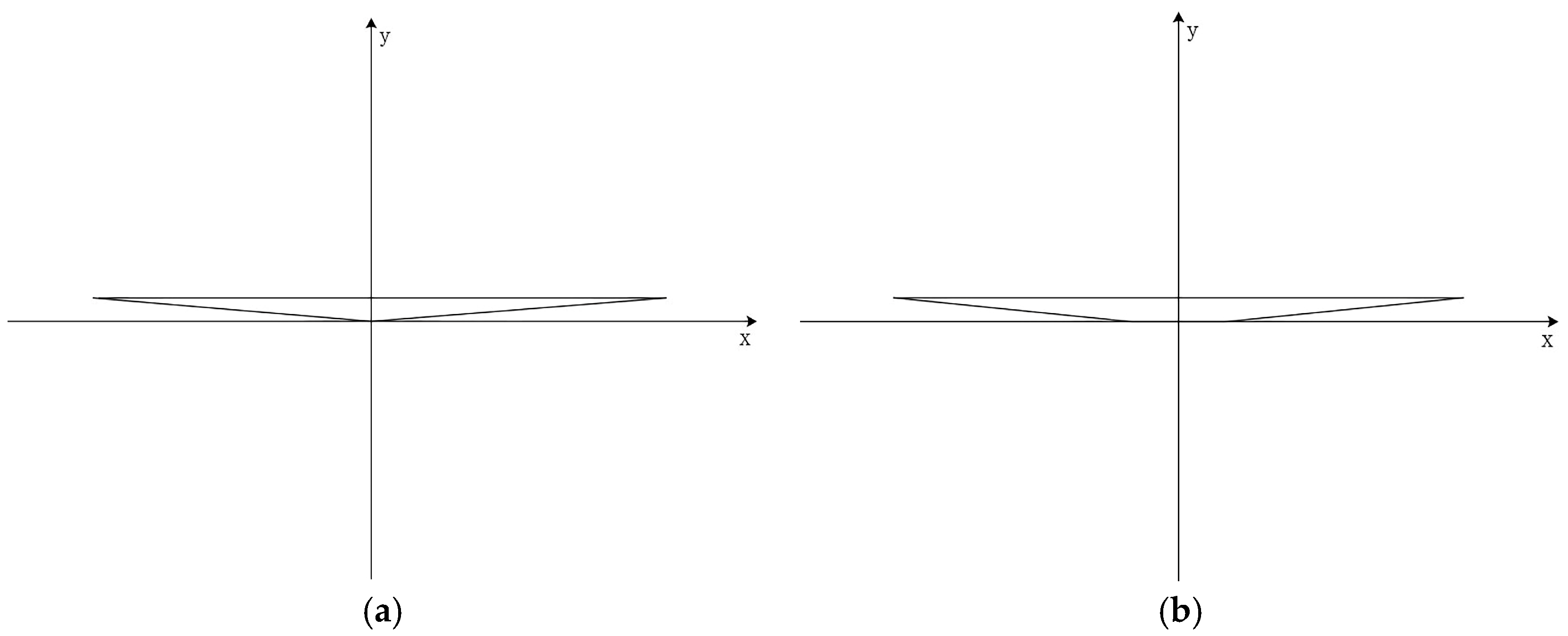
In this study, a simulation of an arc-shaped river section, located in the middle reaches of the Yangtze River, was conducted. The dimensions of the river model shown in Figure 1 were based on this segment, which measures approximately 14,600 m in length and varies between 450 and 900 m in width. Triangles and trapezoids were used as the shape of the river bottom’s cross-section. The entrances to the two different river cross-sections were 800 m wide and the bottoms were 30 m deep, and the slope ratios obtained from the calculations were 0.07 and 0.08, respectively. The average annual discharge of the river is 34,000 m3/s, with an average velocity of 2.83 m2/s for the triangular section and 2.78 m2/s for the trapezoidal section, as obtained from the simulation at the entrance. The accuracy of the model’s calculation results was increased using meshing in Fluent Meshing, which comes from Fluent’s meshing software. A hexahedral grid was used for the river simulation due to the variation in hydraulic elements along the river edge and the high grid density in the vicinity. This grid could improve the accuracy of the numerical calculation results of the model. The computational area under these conditions contained 887,893 cells and 4,819,446 grid nodes.
Additionally, a straight channel was created for comparison with the curved channel. Because the river water temperature is similar to the air temperature, the water temperature was assumed to be 20 °C, in which the hydraulic gradient was 5.6 × 10⁻¹¹ and the kinematic viscosity was 1.01 × 10⁻⁶ m2/s [36]. The cross-section and slope ratios were the same as those for the curved rivers. The cross-sections are shown in Figure 2:
Inland waterways are usually suitable for steady-state analysis due to steady flow velocities [37]. The VOF model was chosen and q w was set to 1 in Equation (2). Using Equations (3), (4) and (5), the turbulent kinetic energy and dissipation rates in the simulation were calculated to be 0.28 m2∕s2 and 0.38 m2∕s3, respectively. The effect of roughness on the river wall was ignored, and the standard wall function method was employed in the near-wall region. Numerical calculations were performed using the finite volume method with discrete differential equations. The SIMPLE algorithm was used to solve the pressure–flow velocity coupling problem. A first-order windward format was used as the discrete format.
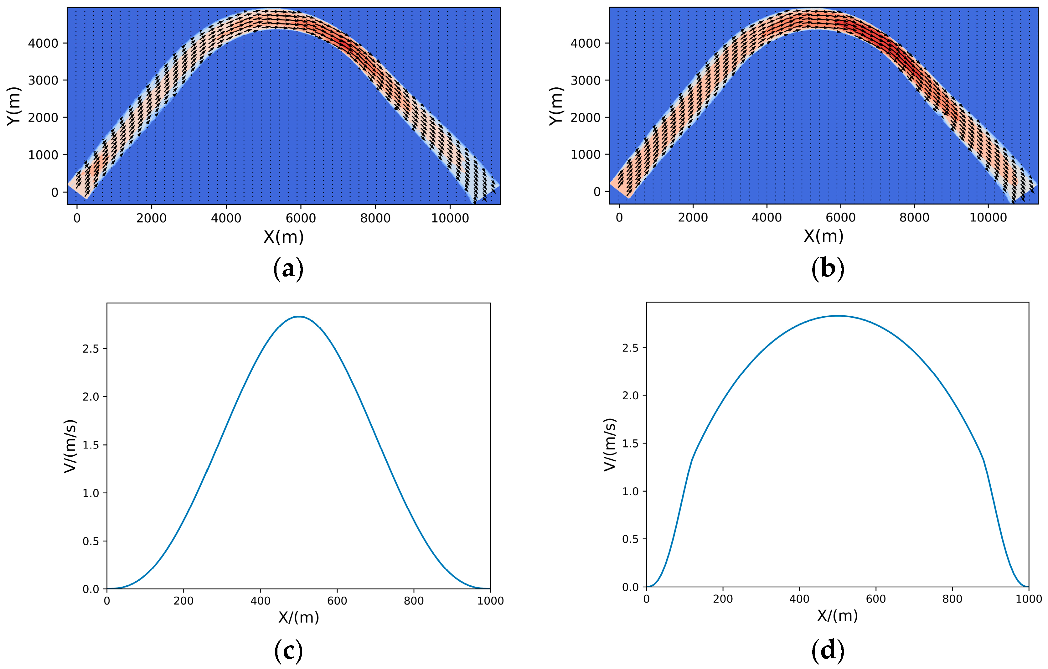
To conduct post-processing of the simulation data, the velocity data at each point on the river surface were obtained via the grid node and exported to generate a CSV file. The interpolation sub-module of the SciPy library in Python was then used to perform interpolation calculations to obtain two flow-field images. Two flow-velocity maps were obtained by solving straight-channel Equation (1). The flow velocities on the triangular section of the curved and straight channels are presented in Figure 3a,c, and the flow velocities of the two channels on the trapezoidal section are depicted in Figure 3b,d.
Figure 3 clearly demonstrates that the flow rate was higher at the center of the river and lower near its sides. Notably, the fastest flow rate was observed at the river bend, which is consistent with the expected flow field dynamics. These model results have important implications for studying the flow behavior of oil spills on river surfaces, in accordance with the laws governing fluid dynamics.
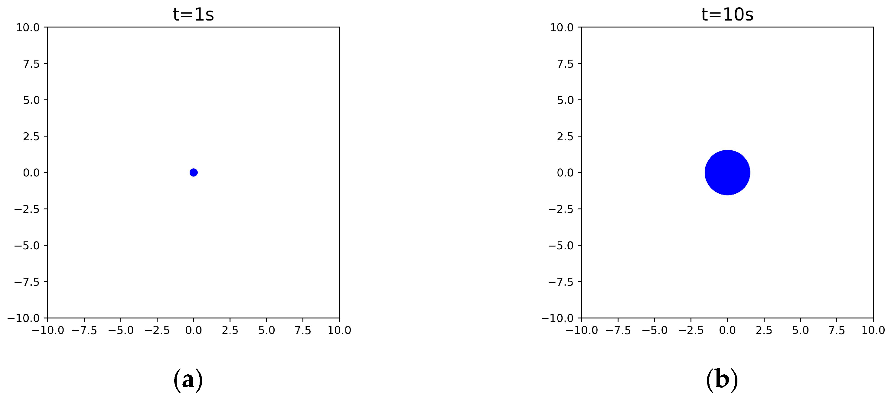
The oil particles were defined in Python using Equation (6). The surface tension expansion phase coefficient m in the equation was empirically determined as 2.3, whereas the surface tension σ was calculated as 0.0146 N∕m [35]. The variation in particle expansion with time is shown in Figure 4. The flow direction and velocity are different for each location in the flow field. Therefore, the perimeter of the oil particles was divided evenly into equal aliquots with the same number of particles. The displacement of each point on the oil particles was derived using Equation (7), and the shape of the oil particles was also changed. Due to the problems of a large amount of data and slow search speed, the kd-tree algorithm was used. The algorithm was mainly used to search data near the current point, so the oil particles could be used to obtain the velocity and direction of the flow field at the next position. The point of the oil particles stopped moving when the surrounding flow rate was 0 m/s. Additionally, a small offset value was added to the oil particles at each movement to avoid the particles overlapping. Due to each particle representing a certain amount of oil, density was defined as the number of oil particles. A higher number of oil particles indicates higher density. The term “collision” refers to “ship collision” in this study.

3.2. Simulation Results of a Continuous Oil Spill

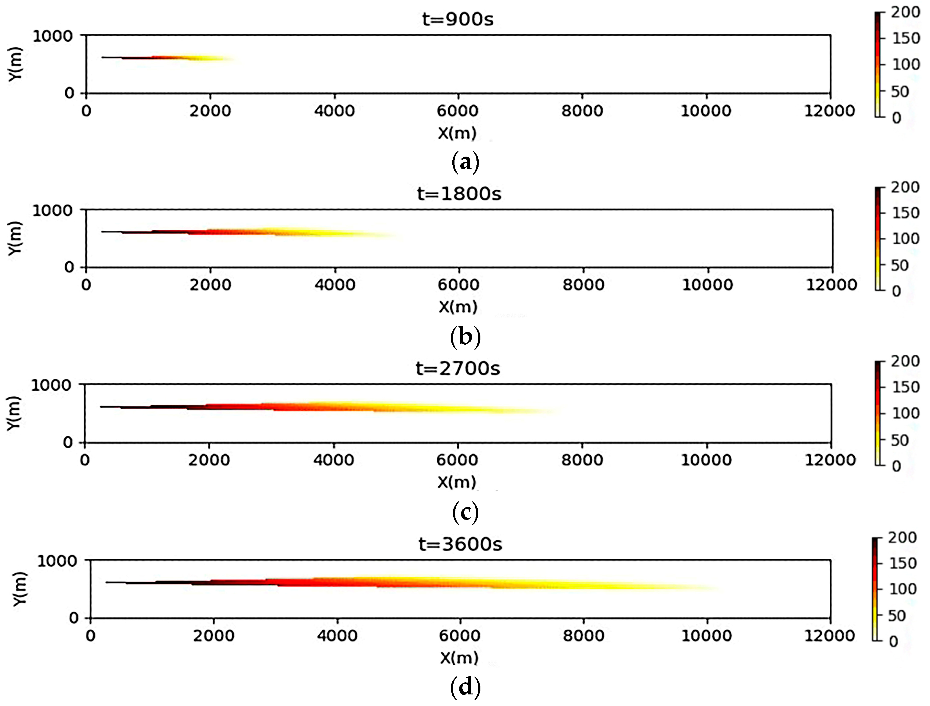
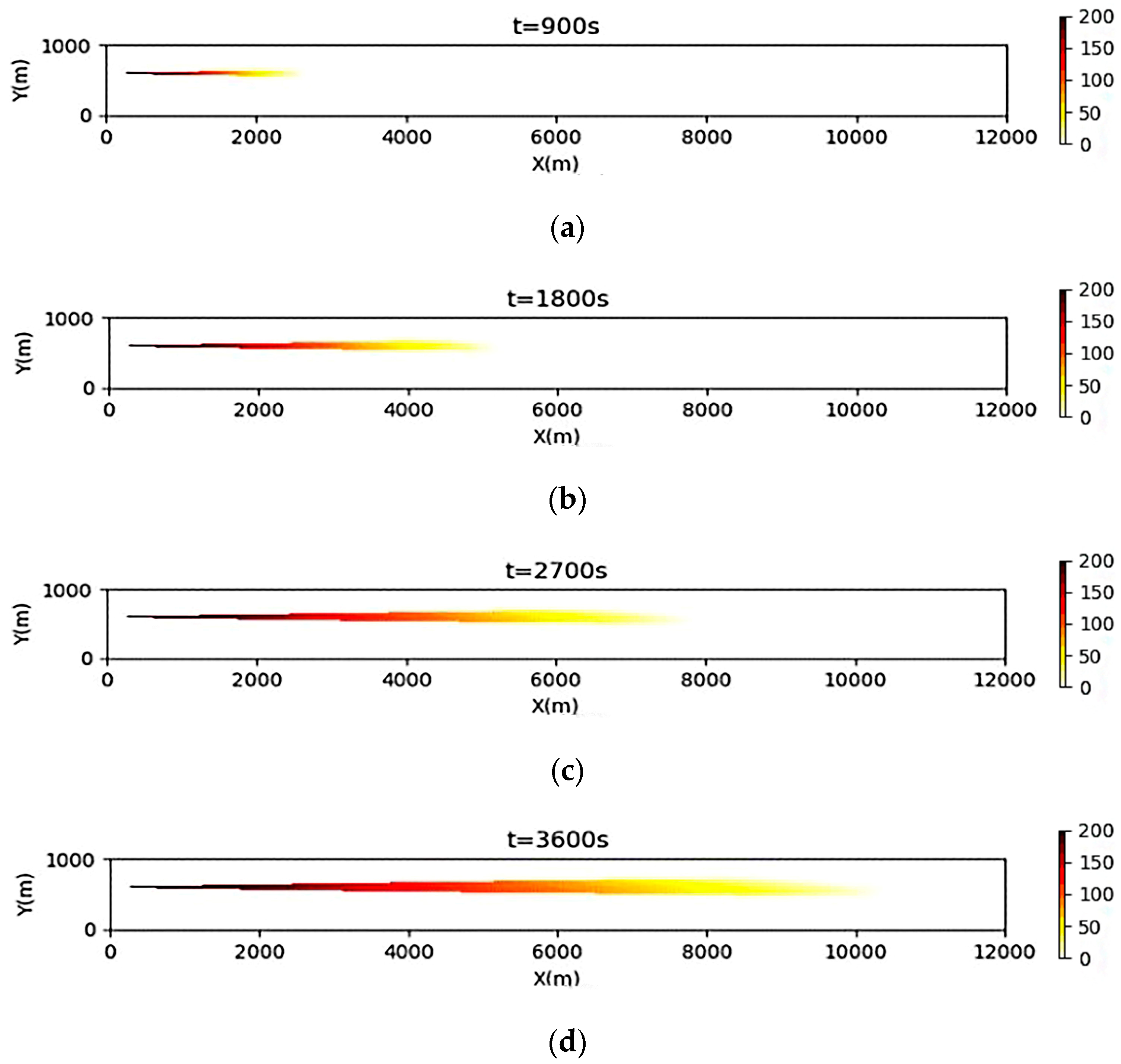
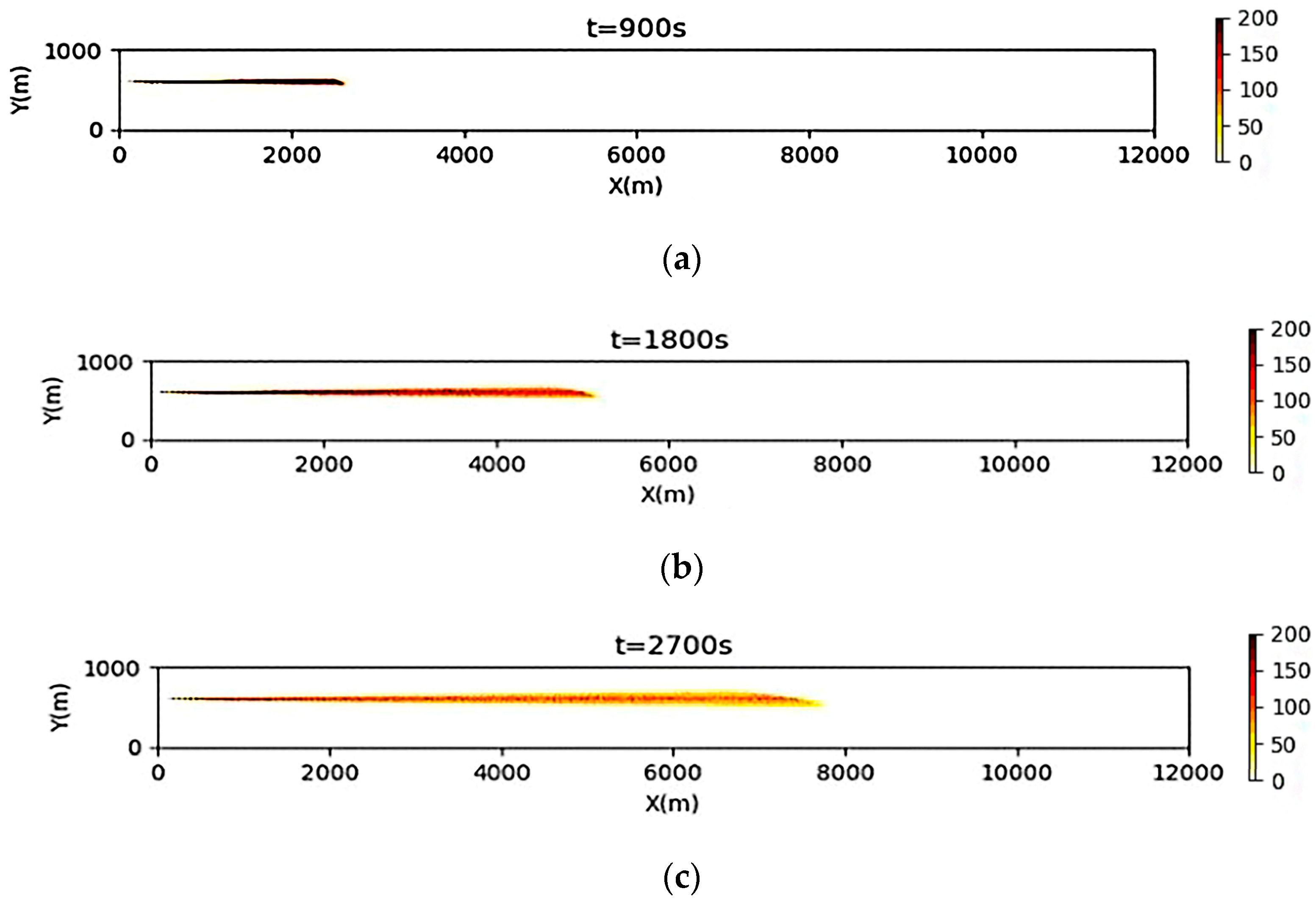
The flow field in a straight channel with two distinct cross-sections was obtained by solving the equations presented above. The ongoing oil spill caused by the ship was assumed to have occurred in the middle. The simulation results for 900, 1800, 2700 and 3600 s were obtained as shown in the figure below.
The continuous oil spill results in a straight channel with a triangular cross-section for scenario 1 are shown in Figure 5. Four time points were selected for comparison. As time progresses, it is observed that the oil spill becomes progressively shallower from left to right and the number of particles changes from 200 to 0, indicating a decrease in its concentration. Furthermore, there is an increase in the length of the oil spill over time. Based on observations at the 2000 m location, the particle number changes from 50 to 175, which indicates a drift of the oil spill to the right with the current. Moreover, in comparing (d) and (b) at the 4000 m position, it can be observed that oil spreads more slowly laterally.
A trapezoidal cross-section of scenario 2 with continuous oil spills under a straight path is shown in Figure 6. Similarly, four time points were selected for comparison, and the same experimental results were obtained as in scenario 1 with respect to the density. However, there is a notable difference between the two figures. In scenario 1, the front end of the oil spill is more elongated and lateral expansion is not apparent. In contrast, the lateral extension of the front end of the oil spill in scenario 2 is more pronounced. Moreover, the extent of the oil spill is more extensive than in scenario 1.
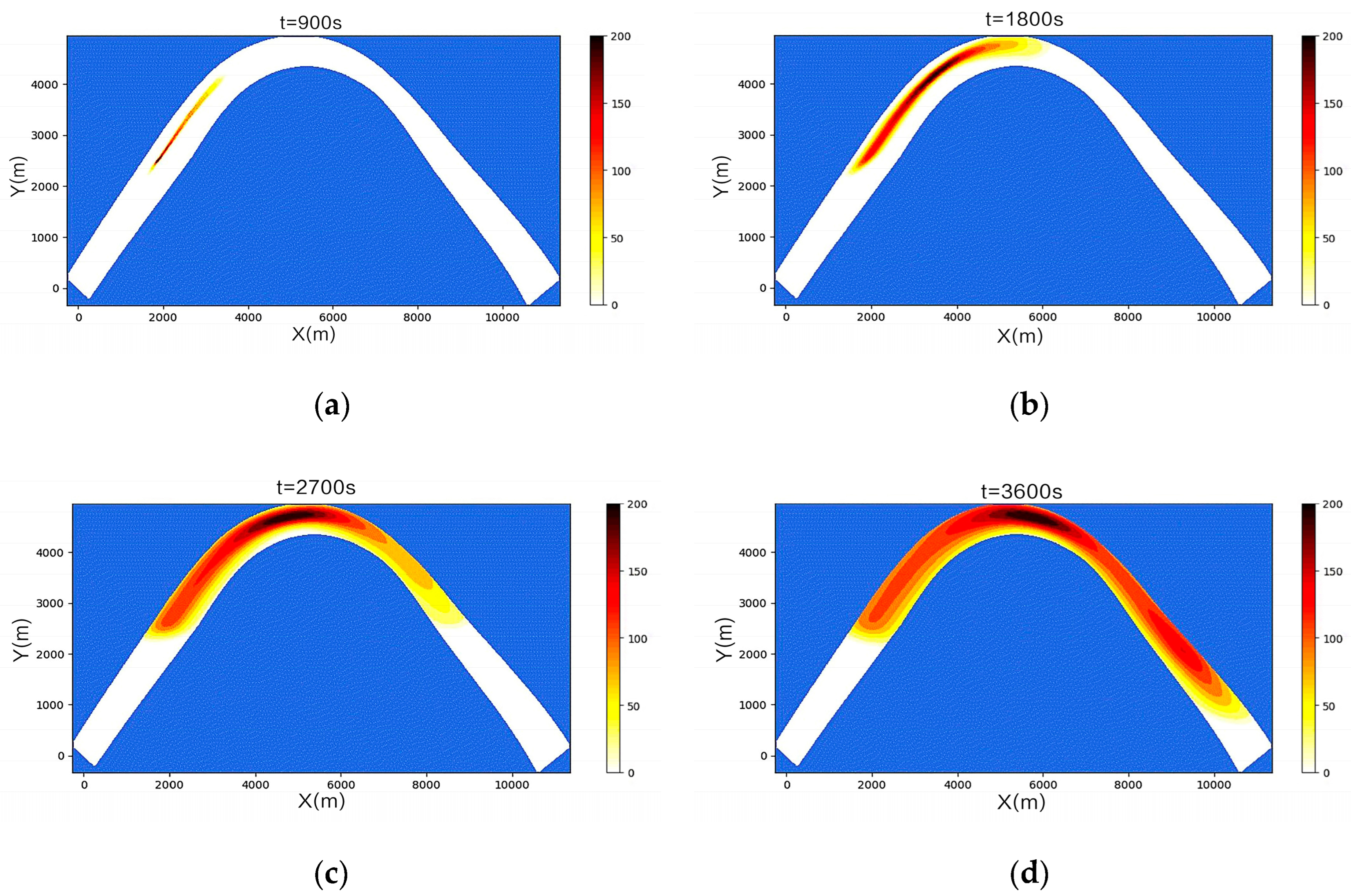
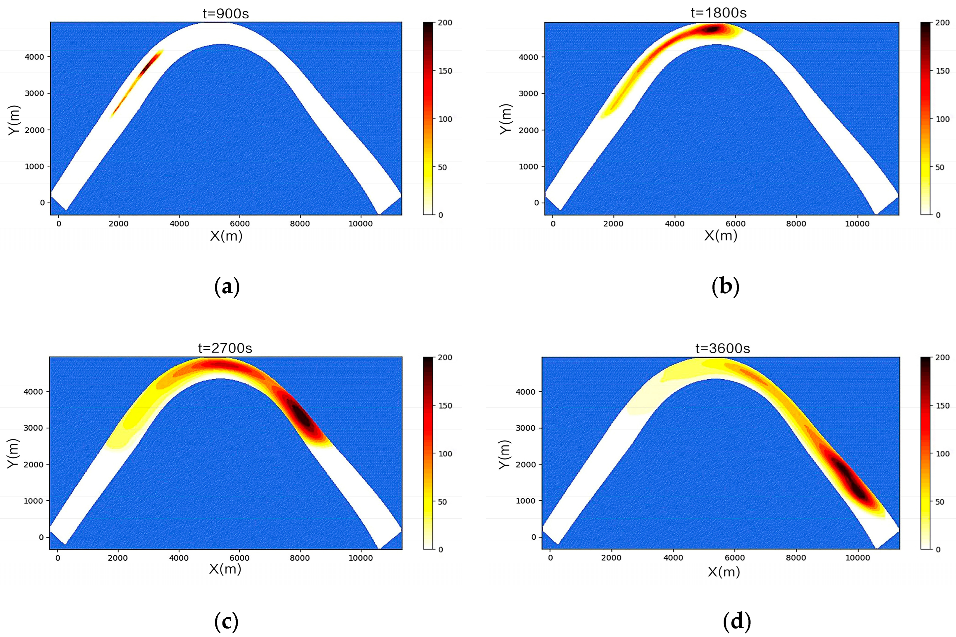
The continuous oil spill scenario 3, under a triangular cross-section within a curved channel, is depicted in Figure 7. During the first 900 s, the highest oil concentration is observed at the initial point. However, the graph at 1800 s shows that the location of the maximum oil spill concentration changed. This was caused by the accumulation of the water-scouring effect and the expansion of oil particles. The flow velocity is the highest after the bend owing to the curvature, and gradually slows as the channel becomes straighter. An increase in density is caused by the accumulation of oil particles, which are affected by the velocity.
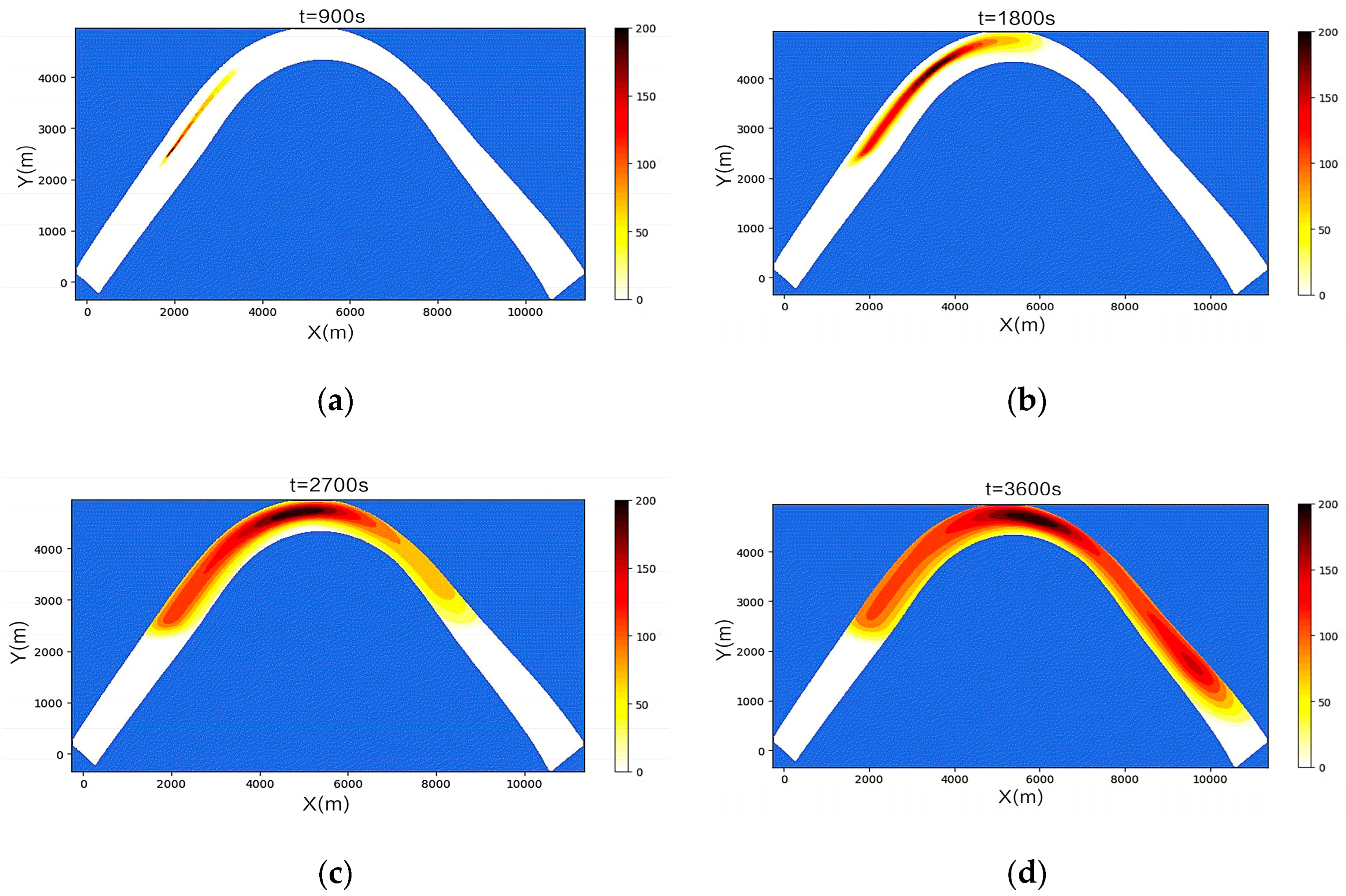
Scenario 4, a continuous oil spill in a curved channel with a trapezoidal cross-section, is illustrated in Figure 8 within the same simulation range as Figure 7. Notably, the position of the maximum density is observed at the onset at 900 s, while it shifts at 1800 s. The maximum density is the maximum number of particles and is represented by the darkest color. However, there is a significant increase in oil density at the front end of the spill at 3600 s, with the deepening range in scenario 4 being greater than that observed in scenario 3. The oil spill in the curved channel with a trapezoidal section has a larger area than that in the triangular channel but a slower rate.
In scenario 1, a straight channel with a triangular section is depicted, whereas in scenario 3, a curved channel with a triangular section is displayed. Similar behaviors are exhibited by the two scenarios at 900 s. However, the emergence of the curved channel leads to alterations in the water flow velocity after 1800 s, causing discrepancies between the two figures. Over time, a shift and further movement away from its original location are observed in the highest-density region in scenario 3. Additionally, the lateral dispersion of oil spills is much more pronounced under the influence of curved channels than that of straight channels. At the tip of the curved channel, the oil spill shape is transformed into an ellipse as opposed to the triangular shape observed in the straight channel. These findings are further corroborated by scenario 2, which demonstrates the significant impact of curved channels on oil spills. In summary, the experimental results clearly indicate that curved channels have a significant influence on the behavior of oil spills.

3.3. Simulation Results of a One-Time Oil Spill

In the event of a ship collision that would result in an oil spill in a river, it is important to understand the dynamics of the oil slick as it moves with the current. To simulate this, diagrams of oil spills with different channel shapes and cross-sections are presented.
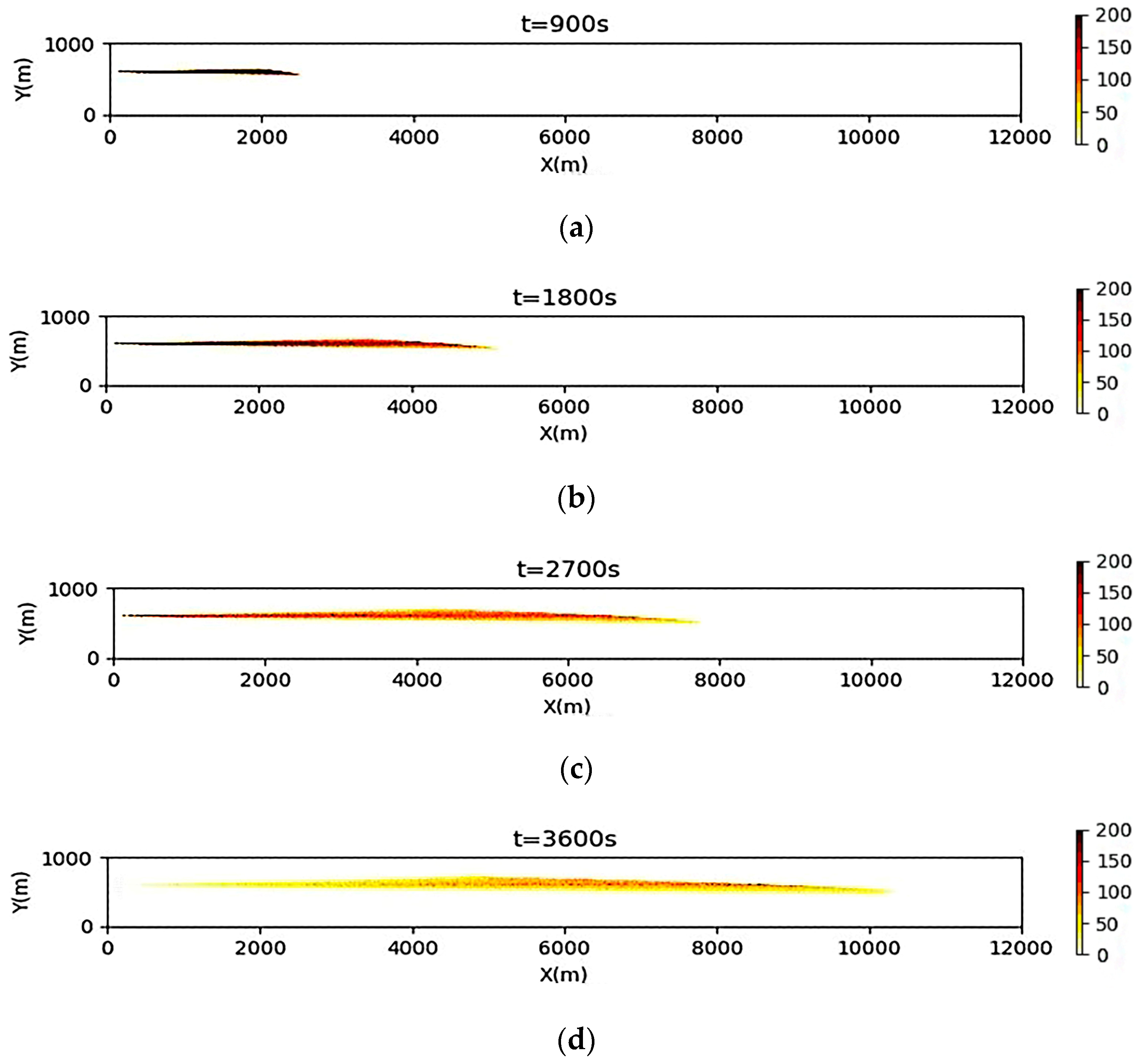
The behavior of the oil spill caused by a collision in a straight channel with a triangular cross-section in scenario 5 is illustrated in Figure 9. It can be inferred from the results that an overall high density was displayed by the oil spill, and a small area of lower density was observed around it at 900 s. However, the experimental results were not significant. A section with a lower density was observed at the front end of the oil spill because of the faster flow rate in that region at 1800 s. Subsequently, a notable reduction in the density was observed at 2700 s as the oil spill gradually spread over the entire channel. Finally, the overall density of the oil spill decreased significantly, with the densities at the front and rear ends being lower than those within the spill.
The behavior of the oil spill caused by a collision in the straight channel under the trapezoidal shape in scenario 6 is depicted in Figure 10. The front-end position appeared gentler compared with that of scenario 5, with a similar overall effect at 900 s. The internal density of the oil spill was higher than the surrounding density, and the oil spill affected a larger area than the oil spill under the triangular cross-section at 1800 s. The overall density of the oil spill was lower than that of the triangular cross-section at 2700 s. Finally, the front-end density was slightly higher than the back-end density, and the density at the back-end of the oil spill was almost negligible.
The results of the oil spill from the collision in the curved channel with a triangular cross-section in scenario 7 are shown in Figure 11. The results revealed that the highest concentration of the oil spill was not at the forefront, but rather, some distance from it. The trajectory of the oil spill from the collision in the channel is shown, and numerous particles are still present, moving with the water flow. Particle build-up was detected at the bend location at 2700 s. Owing to the effect of the bend flow velocity, several oil particles were reassembled into one piece, with the deepest density emerging at the front at 3600 s. The density gradually decreased towards the tail owing to the effect of water scouring.
The results of the oil spill from the collision in the curved channel with a trapezoidal cross-section exhibited in scenario 8 are shown in Figure 12. The results observed in the first 1800 s are similar to those in scenario 7. However, the number of oil particles at the front end and bend locations was smaller and they were less extensive than those observed in Figure 11 at 2700 s. The number of particles in the middle section was around 47 at 3600 s. Additionally, the front of the oil possessed more particles, which were more aggregated. However, the impact range was smaller than that observed in scenario 7.
As can be seen in scenario 5, the oil spill occurred in a straight channel, whereas the same accident was presented in a curved channel with a triangular cross-section in scenario 7. A comparison of the two figures showed that the flow velocity near the curved channel was faster at 900 s, which resulted in an overall density that was no longer uniform. However, the density at the front end remained higher than that at the back end. The lateral diffusion in the curved channel was more pronounced at 1800 s. Oil particles accumulated owing to the flow of water in the curved channel, which led to an increasingly severe oil spill impact when comparing the results at 2700 and 3600 s. These findings are further supported by a comparison of scenario 6 and scenario 8.
The above results clearly demonstrate that oil particles moved in the direction of the water flow through the action of the water flow. Notably, the influence of water flow was more significant than that of oil particle diffusion. The distribution area of the oil particles expanded, and the characteristics of the strip distribution are shown. When comparing the plots under the flow fields of the two different river bottom cross-sections, the oil spill size under the trapezoidal flow field was more significant than that under the triangular flow field. However, the oil spill speed was slightly slower. In addition, the maximum densities of the simulated and experimental flow fields varied, which can be attributed to the change in flow velocity owing to the presence of the bend. Specifically, the flow velocity gradually increased at the bend and decreased in the straight channel, which resulted in a change in the location of the maximum oil spill density. Moreover, the oil particles drifted and aggregated over time due to the decreased flow rate.

4. Discussion

The Yangtze River is the largest river in China and the third largest river globally, containing diverse habitats and ecosystems [38]. In addition, its economic status is critical and it plays a strategic role in the development of China’s inland regions [39]. This status has contributed to the rapid development of ports along the river’s shores, which now constitute more than 40% of China’s gross domestic product (GDP) [40]. However, the traditional economy-oriented development model has overlooked the importance of environmental protection and resource efficiency owing to the rapid growth of the Yangtze River Economic Zone [41]. This has led to an increase in oil spill pollution incidents [42], which negatively impact marine life and the stability of cities along rivers [43,44]. Owing to the increasingly stringent ecological and environmental protection regulations that have been enacted [45], a method to properly simulate Yangtze River oil spills is urgently needed. Therefore, accurate river models are essential for simulating oil spill dispersion and drift to predict the size and location of oil spills in the Yangtze River.
Currently, most research on oil spills has focused on oceans and bays [46,47], whereas this study focused on inland rivers that have previously received less attention. Li et al. [48] found that data quality affects oil spill simulation, so the data on flow fields was improved using interpolation in this study. Jiang et al. [49] studied only one type of oil spill accident, whereas this study simulated two types of inland oil spill to better understand oil spills through comparison. In addition, Bi and Si [50] conducted oil spill simulation but did not compare the effects of flow fields with different channel shapes and cross-sections on oil spills. This represents a lack of reference value for simulating oil spills at different locations in the channel. Therefore, oil spills under flow fields with different channel shapes and cross-sections in inland rivers were simulated to fill this gap.
The results of this study may assist in identifying instances of inland oil spill pollution. Significant variations in the oil particles at the bend location were shown in the results of the simulation experiment. The importance of establishing an accurate early warning system for pollution caused by Yangtze River shipping is highlighted by this finding. This system can be used for decision-making, such as developing oil spill plans, promoting pollution prevention, and determining responsibility for managing pollution incidents. In addition, oil spills under trapezoidal cross-sections can spread more widely. It is therefore necessary to establish additional monitoring stations in the Yangtze River Basin so that oil spills can be detected more quickly in the trapezoidal section. Maritime departments can identify the sources of oil spills in inland rivers through a combination of this research and GIS. This will accelerate the management and layout of emergency pollution events, as well as assisting in determining responsibility for managing oil spill incidents. The visualized oil spill simulation results can be used for environmental education, providing the public with a greater understanding of the environmental consequences of oil spills and raising public awareness of the importance of environmental protection.
This oil spill study still has some limitations. Specifically, it did not take into account factors such as temperature variations, wind and other variations in oil. In addition, the oil spill simulation could have been affected to a certain degree by discrepancies between the flow field assumptions and the actual situation. Additionally, the diffusion coefficient of the oil particle model was taken from the empirical value, which causes some uncertainty.

5. Conclusions

In this study, the flow field of the Yangtze River was established using a VOF multiphase flow model and an open-channel equation, and a two-dimensional oil spill dispersion drift model was constructed by combining the oil particle models. Furthermore, two oil spill accidents were simulated, and the results of the eight scenarios were compared. The results suggested that striated characteristics were developed by the oil owing to water movement. In addition, oil spills on rivers with trapezoidal cross-sections were more extensive than those with triangular cross-sections. The density of the oil particles varied with flow time owing to the different flow rates at different locations, which resulted in different levels of aggregation at each spot. The effect of a curved channel was critical because it led to the diffusion of oil particles, which were more pronounced than in a straight channel and became biased toward the side of the curve.
Future research should focus on a comprehensive analysis that incorporates wind- and oil-type factors. In addition, combining GIS for real-time monitoring and creating an Internet database would significantly enhance experimental accuracy. Moreover, oil spills in the upper and lower reaches of the river should be considered to improve the simulation accuracy.

Author Contributions

Conceptualization, G.Y. and J.D.; methodology, C.K. and Y.S.; software, H.Y. and C.K.; validation, H.Y. and J.D.; formal analysis, J.D.; resources, H.Y. and C.K.; data curation, H.Y.; writing—original draft preparation, C.K. and G.Y.; writing—review and editing, C.K. and Y.S. All authors have read and agreed to the published version of the manuscript.

Funding

This work was supported by the National Natural Science Foundation of China (NSFC) under Grant No. 52271369.

Institutional Review Board Statement

Not applicable.

Informed Consent Statement

Not applicable.

Data Availability Statement

Not applicable.

Conflicts of Interest

The authors declare no conflict of interest.

References

  1. Gan, L.; Yan, Z.; Zhang, L.; Liu, K.; Zheng, Y.; Zhou, C.; Shu, Y. Ship path planning based on safety potential field in inland rivers. Ocean Eng. 2022, 260, 111928. [Google Scholar] [CrossRef]
  2. Shu, Y.; Zhu, Y.; Xu, F.; Gan, L.; Lee, P.T.-W.; Yin, J.; Chen, J. Path planning for ships assisted by the icebreaker in ice-covered waters in the Northern Sea Route based on optimal control. Ocean Eng. 2023, 267, 113182. [Google Scholar] [CrossRef]
  3. Bayazit, O.; Kaptan, M. Evaluation of the risk of pollution caused by ship operations through bow-tie-based fuzzy Bayesian network. J. Clean. Prod. 2023, 382, 135386. [Google Scholar] [CrossRef]
  4. Shu, Y.; Wang, X.; Huang, Z.; Song, L.; Fei, Z.; Gan, L.; Xu, Y.; Yin, J. Estimating spatiotemporal distribution of wastewater generated by ships in coastal areas. Ocean. Coast. Manag. 2022, 222, 106133. [Google Scholar] [CrossRef]
  5. Yu, Y.; Chen, L.; Shu, Y.; Zhu, W. Evaluation model and management strategy for reducing pollution caused by ship collision in coastal waters. Ocean. Coast. Manag. 2021, 203, 105446. [Google Scholar] [CrossRef]
  6. Liu, K.; Yu, Q.; Yuan, Z.; Yang, Z.; Shu, Y. A systematic analysis for maritime accidents causation in Chinese coastal waters using machine learning approaches. Ocean. Coast. Manag. 2021, 213, 105859. [Google Scholar] [CrossRef]
  7. Yang, Z.; Chen, Z.; Lee, K. Development and testing of a 2D offshore oil spill modeling tool (OSMT) supported by an effective calibration method. Mar. Pollut. Bull. 2023, 188, 114696. [Google Scholar] [CrossRef]
  8. Kahkashan, S.; Wang, X.; Ya, M.; Chen, J.; Wu, Y.; Cai, Y.; Saleem, M.; Inam, A.; Aftab, J. Evaluation of marine sediment contamination by polycyclic aromatic hydrocarbons along the Karachi coast, Pakistan, 11 years after the Tasman Spirit oil spill. Chemosphere 2019, 233, 652–659. [Google Scholar] [CrossRef]
  9. Scarlett, A.G.; Nelson, R.K.; Gagnon, M.M.; Holman, A.I.; Reddy, C.M.; Sutton, P.A.; Grice, K. MV Wakashio grounding incident in Mauritius 2020: The world’s first major spillage of Very Low Sulfur Fuel Oil. Mar. Pollut. Bull. 2021, 171, 112917. [Google Scholar] [CrossRef]
  10. McClenachan, G.; Turner, R.E. Disturbance legacies and shifting trajectories: Marsh soil strength and shoreline erosion a decade after the Deepwater Horizon oil spill. Environ. Pollut. 2023, 322, 121151. [Google Scholar] [CrossRef]
  11. Chen, J.; Di, Z.; Shi, J.; Shu, Y.; Wan, Z.; Song, L.; Zhang, W. Marine oil spill pollution causes and governance: A case study of Sanchi tanker collision and explosion. J. Cleaner Prod. 2020, 273, 122978. [Google Scholar] [CrossRef]
  12. Fei, Y.; Chen, J.; Wan, Z.; Shu, Y.; Xu, L.; Li, H.; Bai, Y.; Zheng, T. Crude oil maritime transportation: Market fluctuation characteristics and the impact of critical events. Energy Rep. 2020, 6, 518–529. [Google Scholar] [CrossRef]
  13. Espedal, H.A. Satellite SAR oil spill detection using wind history information. Int. J. Remote Sens. 1999, 20, 49–65. [Google Scholar] [CrossRef]
  14. Gautama, B.G.; Longépé, N.; Fablet, R.; Mercier, G. Assimilative 2-D Lagrangian Transport Model for the Estimation of Oil Leakage Parameters From SAR Images: Application to the Montara Oil Spill. IEEE J. Sel. Top. Appl. Earth Obs. Remote Sens. 2016, 9, 4962–4969. [Google Scholar] [CrossRef]
  15. Conceição, M.R.; de Mendonça, L.F.; Lentini, C.A.; da Cunha Lima, A.T.; Lopes, J.M.; de Vasconcelos, R.N.; Gouveia, M.B.; Porsani, M.J. SAR Oil Spill Detection System through Random Forest Classifiers. Remote Sens. 2021, 13, 2044. [Google Scholar] [CrossRef]
  16. Huby, A.A.; Alubady, R.; Sagban, R. Oil Spill Segmentation from SAR Images Using Deep Neural Networks. In Proceedings of the 2022 International Symposium on Multidisciplinary Studies and Innovative Technologies (ISMSIT), Ankara, Turkey, 20–22 October 2022; pp. 282–287. [Google Scholar]
  17. Goyal, V.; Shukla, A. A New Optimized GA-RBF Neural Network Algorithm for Oil Spill Detection in SAR Images. In Advances in Computer, Communication and Computational Sciences, Proceedings of the IC4S 2019, Bangkok, Thailand, 11―12 October 2019; Springer: Berlin/Heidelberg, Germany, 2021; pp. 987–999. [Google Scholar]
  18. Ma, X.; Xu, J.; Wu, P.; Kong, P. Oil Spill Detection Based on Deep Convolutional Neural Networks Using Polarimetric Scattering Information From Sentinel-1 SAR Images. IEEE Trans. Geosci. Remote Sens. 2022, 60, 4204713. [Google Scholar] [CrossRef]
  19. Prants, S.V.; Budyansky, M.V.; Fayman, P.A.; Uleysky, M.Y.; Didov, A.A. Lagrangian Oil Spill Simulation in Peter the Great Bay (Sea of Japan) with a High-Resolution ROMS Model. Pure Appl. Geophys. 2023, 180, 551–568. [Google Scholar] [CrossRef]
  20. Dąbrowska, E.; Kołowrocki, K. Stochastic determination of oil spill domain at Gdynia Port water area. In Proceedings of the 2019 International Conference on Information and Digital Technologies (IDT), Seoul, Republic of Korea, 18–19 January 2019; pp. 92–97. [Google Scholar]
  21. Ghaly, M.N.; Badr, N.E.; Omar, M.Y.; Amin, H.A. Risk Assessment of Oil Spills at Alexandria Port, Alexandria, Egypt. In Advanced Intelligent Systems for Sustainable Development (AI2SD’2019) Volume 3, Proceedings of the Advanced Intelligent Systems for Sustainable Development Applied to Environment, Industry and Economy, Marrakech, Morocco, 8–11 July 2019; Springer: Berlin/Heidelberg, Germany, 2020; pp. 569–585. [Google Scholar]
  22. Kvočka, D.; Žagar, D.; Banovec, P. A Review of River Oil Spill Modeling. Water 2021, 13, 1620. [Google Scholar] [CrossRef]
  23. Jiang, P.; Tong, S.; Wang, Y.; Xu, G. Modelling the oil spill transport in inland waterways based on experimental study. Environ. Pollut. 2021, 284, 117473. [Google Scholar] [CrossRef]
  24. Yu, D.; Wang, J.; Cao, Q.; Zhang, X.; Liu, X. Numerical Simulation of Crude Oil Spreading in a Complex River Channel. In Proceedings of the International Pipeline Conference, Online, 28–30 September 2020; p. V003T004A010. [Google Scholar]
  25. Wang, Z.; Fingas, M.; Lambert, P.; Zeng, G.; Yang, C.; Hollebone, B. Characterization and identification of the Detroit River mystery oil spill (2002). J. Chromatogr. A 2004, 1038, 201–214. [Google Scholar] [CrossRef]
  26. Da Cunha, A.C.; De Abreu, C.H.M.; Crizanto, J.L.P.; Cunha, H.F.A.; Brito, A.U.; Pereira, N.N. Modeling pollutant dispersion scenarios in high vessel-traffic areas of the Lower Amazon River. Mar. Pollut. Bull. 2021, 168, 112404. [Google Scholar] [CrossRef]
  27. Chen, Y. Development of an oil spill model adaptable to exposure and submergence conversion of tidal flats: A case study in the Changjiang Estuary. Mar. Pollut. Bull. 2021, 171, 112715. [Google Scholar] [CrossRef]
  28. Kim, C.-S.; Cho, Y.-K.; Choi, B.-J.; Jung, K.T.; You, S.H. Improving a prediction system for oil spills in the Yellow Sea: Effect of tides on subtidal flow. Mar. Pollut. Bull. 2013, 68, 85–92. [Google Scholar] [CrossRef]
  29. Sun, D.-L.; Xu, J.-L.; Wang, L. Development of a vapor–liquid phase change model for volume-of-fluid method in FLUENT. Int. Commun. Heat Mass Transf. 2012, 39, 1101–1106. [Google Scholar] [CrossRef]
  30. Hopf, L. Turbulenz bei einem Flusse. Ann. Phys. 1910, 337, 777–808. [Google Scholar] [CrossRef] [Green Version]
  31. Launder, B.E.; Spalding, D.B. Lectures in Mathematical Models of Turbulence; Academic Press: Cambridge, MA, USA, 1972. [Google Scholar]
  32. Shih, T.-H.; Zhu, J.; Lumley, J.L. A new Reynolds stress algebraic equation model. Comput. Methods Appl. Mech. Eng. 1995, 125, 287–302. [Google Scholar] [CrossRef] [Green Version]
  33. Reed, M.; Aamo, O.M.; Daling, P.S. Quantitative analysis of alternate oil spill response strategies using OSCAR. Spill Sci. Technol. Bull. 1995, 2, 67–74. [Google Scholar] [CrossRef]
  34. Board, T.R.; Council, N.R. Oil in the Sea III: Inputs, Fates, and Effects; The National Academies Press: Washington, DC, USA, 2003; p. 277. [Google Scholar]
  35. Fay, J.A. Physical Processes in the Spread of Oil on a Water Surface. Int. Oil Spill Conf. Proc. 1971, 1971, 463–467. [Google Scholar] [CrossRef]
  36. Lu, N.; Zhang, C.; Hillel, D. Water properties☆. In Reference Module in Earth Systems and Environmental Sciences; Elsevier: Amsterdam, The Netherlands, 2023. [Google Scholar]
  37. Poff, N.L. Section Introduction: Structures and Functions of Inland Water–Rivers. Encycl. Inland Waters 2022, 2, 235–236. [Google Scholar]
  38. Wang, Q.; Xu, H.; Yin, J.; Du, S.; Liu, C.; Li, J.-y. Significance of the great protection of the Yangtze River: Riverine input contributes primarily to the presence of PAHs and HMs in its estuary and the adjacent sea. Mar. Pollut. Bull. 2023, 186, 114366. [Google Scholar] [CrossRef]
  39. Wu, Z.; Woo, S.-H.; Lai, P.-L.; Chen, X. The economic impact of inland ports on regional development: Evidence from the Yangtze River region. Transp. Policy 2022, 127, 80–91. [Google Scholar] [CrossRef]
  40. Zhang, Q.; Yang, D.; Chen, Y. Port integration on the Yangtze River: Does it follow an "interest balance" pattern? Transp. Policy 2021, 108, 83–94. [Google Scholar] [CrossRef]
  41. Liu, L.; Yang, Y.; Liu, S.; Gong, X.; Zhao, Y.; Jin, R.; Duan, H.; Jiang, P. A comparative study of green growth efficiency in Yangtze River Economic Belt and Yellow River Basin between 2010 and 2020. Ecol. Indic. 2023, 150, 110214. [Google Scholar] [CrossRef]
  42. Zhao, J.; Zhao, Y. Synergy/trade-offs and differential optimization of production, living, and ecological functions in the Yangtze River economic Belt, China. Ecol. Indic. 2023, 147, 109925. [Google Scholar] [CrossRef]
  43. Adofo, Y.K.; Nyankson, E.; Agyei-Tuffour, B. Dispersants as an oil spill clean-up technique in the marine environment: A review. Heliyon 2022, 8, e10153. [Google Scholar] [CrossRef]
  44. Xiao, G.; Wang, T.; Luo, Y.; Yang, D. Analysis of port pollutant emission characteristics in United States based on multiscale geographically weighted regression. Front. Mar. Sci. 2023, 10, 1131948. [Google Scholar] [CrossRef]
  45. Lin, B.; Zhang, A. Can government environmental regulation promote low-carbon development in heavy polluting industries? Evidence from China’s new environmental protection law. Environ. Impact Assess. Rev. 2023, 99, 106991. [Google Scholar] [CrossRef]
  46. Ivorra, B.; Gomez, S.; Carrera, J.; Ramos, A.M. A compositional Eulerian approach for modeling oil spills in the sea. Ocean Eng. 2021, 242, 110096. [Google Scholar] [CrossRef]
  47. Zhen, Z.; Li, D.; Li, Y.; Chen, S.; Bu, S. Trajectory and weathering of oil spill in Daya bay, the South China sea. Environ. Pollut. 2020, 267, 115562. [Google Scholar] [CrossRef]
  48. Li, Y.; Brimicombe, A.J.; Ralphs, M.P. Spatial data quality and sensitivity analysis in GIS and environmental modelling: The case of coastal oil spills. Comput. Environ. Urban Syst. 2000, 24, 95–108. [Google Scholar] [CrossRef]
  49. Jiang, P.; Tong, S.; Wang, Y. Establishment and application of oil spill model in inland waterway. In Proceedings of the 6th International Conference on Hydraulic and Civil Engineering, ICHCE 2020, Xi’an, China, 11–13 December 2020. [Google Scholar]
  50. Bi, H.; Si, H. Dynamic risk assessment of oil spill scenario for Three Gorges Reservoir in China based on numerical simulation. Saf. Sci. 2012, 50, 1112–1118. [Google Scholar] [CrossRef]
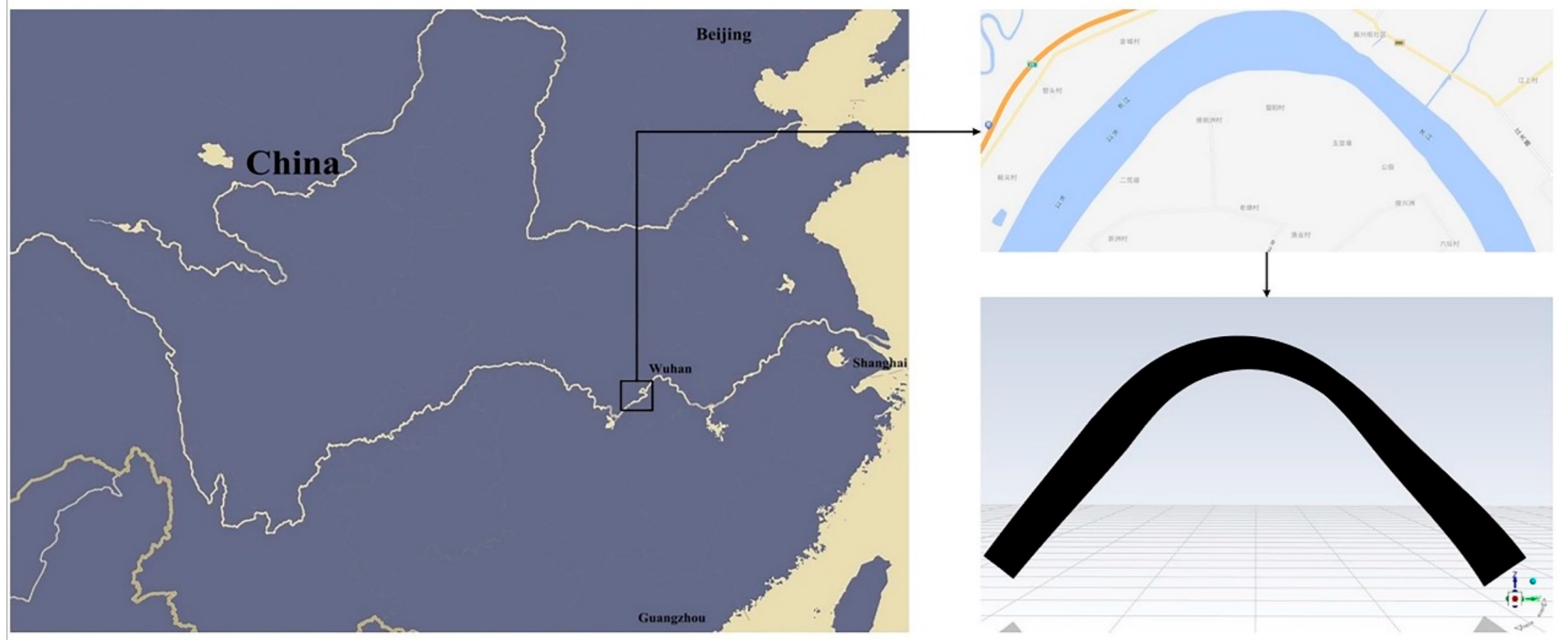
Figure 1. Location as selected from Baidu Maps.
Jmse 11 01294 g001
Figure 2. Two types of cross-section used for the simulation of the Yangtze River: (a) triangular cross-section and (b) trapezoidal cross-section.
Jmse 11 01294 g002
Figure 3. Velocities under different channel shapes and cross-sections: (a) curved and triangular, (b) curved and trapezoidal, (c) straight and triangular and (d) straight and trapezoidal.
Jmse 11 01294 g003
Figure 4. Diffusion changes in the oil particles. Sub-figures (a,b) represent the changes at 1 and 10 s, respectively.
Jmse 11 01294 g004
Figure 5. Continuous oil spills occurring in a straight channel with a triangular cross-section in scenario 1. Sub-figures (a), (b), (c) and (d) represent the situation at 900, 1800, 2700 and 3600 s, respectively.
Jmse 11 01294 g005
Figure 6. Continuous oil spills occurring in a straight channel with a trapezoidal cross-section in scenario 2. Sub-figures (a), (b), (c) and (d) represent the situation at 900, 1800, 2700 and 3600 s, respectively.
Jmse 11 01294 g006
Figure 7. Continuous oil spills occurring in a curved channel with a triangular cross-section in scenario 3. Sub-figures (a), (b), (c) and (d) represent the situation at 900, 1800, 2700 and 3600 s, respectively.
Jmse 11 01294 g007
Figure 8. Continuous oil spills occurring in a curved channel with a trapezoidal cross-section in scenario 4. Sub-figures (a), (b), (c) and (d) represent the situation at 900, 1800, 2700 and 3600 s, respectively.
Jmse 11 01294 g008
Figure 9. One-time oil spills occurring in a straight channel with a triangular cross-section in scenario 5. Sub-figures (a), (b), (c) and (d) represent the situation at 900, 1800, 2700 and 3600 s, respectively.
Jmse 11 01294 g009
Figure 10. One-time oil spills occurring in a straight channel with a trapezoidal cross-section in scenario 6. Sub-figures (a), (b), (c) and (d) represent the situation at 900, 1800, 2700 and 3600 s, respectively.
Jmse 11 01294 g010aJmse 11 01294 g010b
Figure 11. One-time oil spills occurring in a curved channel with a triangular cross-section in scenario 7. Sub-figures (a), (b), (c) and (d) represent the situation at 900, 1800, 2700 and 3600 s, respectively.
Jmse 11 01294 g011
Figure 12. One-time oil spills occurring in a curved channel with a trapezoidal cross-section in scenario 8. Sub-figures (a), (b), (c) and (d) represent the situation at 900, 1800, 2700 and 3600 s, respectively.
Jmse 11 01294 g012
Table 1. Eight different scenarios in the simulation.
ScenariosConditionsChannel ShapesCross-Sections
1ContinuousStraightTriangular
2ContinuousStraightTrapezoidal
3ContinuousCurvedTriangular
4ContinuousCurvedTrapezoidal
5One-timeStraightTriangular
6One-timeStraightTrapezoidal
7One-timeCurvedTriangular
8One-timeCurvedTrapezoidal
Disclaimer/Publisher’s Note: The statements, opinions and data contained in all publications are solely those of the individual author(s) and contributor(s) and not of MDPI and/or the editor(s). MDPI and/or the editor(s) disclaim responsibility for any injury to people or property resulting from any ideas, methods, instructions or products referred to in the content.