Robust Adaptive Backstepping Motion Control of Underwater Cable-Driven Parallel Mechanism Using Improved Linear Model Predictive Control

Abstract

This paper proposes a novel motion-tracking control methodology for an underwater cable-driven parallel mechanism (CDPM) that achieves calculation of dynamic tension constraint values, tension planning, parameter linearization, and motion tracking. The control objective is divided into three sub-objectives: motion tracking, horizontal displacement suppression, and cable-tension restriction. A linear model predictive control (LMPC) method is designed to plan cable tensions for motion-tracking and displacement suppression. The robust adaptive backstepping controller converts cable tension into winch speed based on the joint-space method and command filtering. Moreover, the X−swapping method is used to linearize and identify the time−varying nonlinear parameters. An essential prerequisite for restricting cable tension is to obtain cable-tension constraint values. A novel dynamic minimum tension control (DMTC) method, based on the equivalent control concept, is proposed for this aim. The DMTC can adaptively obtain the lower cable-tension threshold through the platform posture and motion status, anchor distribution position, and cable integrity status. Compared to traditional fixed tension constraint values, DMTC can more effectively cope with sudden changes in cable tension than fixed tension constraints. Finally, several simulations are carried out to verify the effectiveness and robustness of the proposed approach.

1. Introduction

Cable-driven parallel mechanisms (CDPMs) are widely used in engineering fields such as building construction, 3D printing, astronomical telescopes, lifting systems, and underwater tension leg platforms [1,2,3,4]. Compared with rigid link parallel mechanisms, CDPMs employ flexible cables as force transmission and position constraint parts to manipulate an end-effector over a feasible workspace, which leads to higher load-to-weight ratios [5,6,7,8,9,10,11,12].

However, the cable-driven structures also introduce significant challenges to the dynamic control of CDPMs, such as elastic deformation, sagging, and unidirectional force. Researchers have developed several methods to solve these problems, including sliding mode control (SMC), adaptive control, adaptive sliding mode control, fuzzy logic control, and neural networks [13,14,15,16,17].

Due to its effectiveness, simplicity, and disturbance rejection capability, sliding mode control has become a common method for controlling CDPMs. Jia et al. [13] proposed a control strategy that combined second-order sliding mode with synchronization control. The second-order sliding mode method was designed to compensate for the influence of unknown parameters, and the synchronization control method was developed to adjust the tension distribution status between cables. Although the effectiveness of the control scheme was verified by tracking experiments, the chattering phenomena caused by discontinuous control still needed to be solved.

A fuzzy system can be used to enhance the performance of sliding mode control designs by tuning the gains of the main SMC controller [18,19]. Vu et al. [18] proposed an optimal fuzzy-enhanced sliding mode control approach for a Stewart parallel robot platform. The optimal fuzzy method was designed to adaptively tune the slopes of the sliding surfaces and the gains of the switching part of the sliding mode controller; the systematic approach of creating the table of rules of fuzzy systems was proposed to provide the required coefficients of the sliding mode controller, which attained optimum performance and minimum control effort, and eliminated the need for computationally expensive expert systems. Mokhtare et al. [19] designed a linear matrix inequality-based fuzzy fast terminal sliding mode control approach. The linear matrix inequality method was used to obtain control parameters; the fuzzy logic approach was designed to fine-tune the controller parameters and reduce the amplitude of the control signal, which led to a smooth transition between control surfaces and reduced the chattering phenomena.

In addition to solving chattering phenomena, researchers are requested to ensure the convergence of the system states to the equilibrium points in finite time. Alattas et al. [20] proposed a nonsingular terminal sliding mode control strategy and proportional–integral switching surface with a self-tuning algorithm for this issue. As a result, the terminal sliding mode control method had a faster convergence rate than traditional sliding mode control and avoided the singularity problem. At the same time, the self-tuning adaptation law was introduced to tackle the disturbance.

Even though having obtained sound effects, traditional sliding mode control methods still require sufficient prior knowledge, frequently unknown in practice. In order to solve this problem, Mobayen et al. [21] proposed a novel barrier function-based adaptive non-singular terminal sliding mode control methodology for robust stability of disturbed nonlinear systems. The barrier function eliminated the necessity of any prior knowledge about the external disturbance upper thresholds, and the terminal sliding mode control methodology approach forced the state trajectories to converge to a region near the origin in a finite time.

Adaptive control is another essential method for underwater CDPM motion control. A novel adaptive super-twisting nonsingular fast terminal sliding mode (AST-NFTSM) controller with time-delay estimation was proposed to guarantee high-precision trajectory tracking control under complicated unknown uncertainties [22]. The time-delay estimation was carried out to compensate for the remaining lumped system dynamics, an adaptive super-twisting term was applied to ensure fast convergence and strong robustness in the reaching phase, and an NFTSM term was utilized to guarantee fast convergence and high precision in the sliding mode phase. Although exciting results have been obtained with AST-NFTSM control schemes, the tension constraint and coordination control between winches are ignored. Ji et al. [23] proposed a novel adaptive control scheme to simultaneously handle the kinematic and dynamic uncertainties, which performed high-precision tracking tasks. The linear expressions of kinematic and dynamic models and adaptation laws were derived through gradient descent. However, the differences between cables were ignored in the paper. Godbole et al. [24] developed a Rayleigh–Ritz cable model to compensate for the effect of time−varying parameters. The changes in cable mass and stiffness caused by its winding and unwinding around the winches, which were described through the passivity-based adaptive control law, were considered in this model. Moreover, an energy-based model simplification was proposed to facilitate the reduction in the computational load. Wang et al. [25] proposed an adaptive PD control scheme combining a PD controller with an adaptive radial basis function (RBF) neural network. The adaptive PD control was used to track the trajectory of the CDPM end effector, and the RBF neural network control method was used to approximate the parameters. Although good results have been reported with the above works, most control methods require accurate system models and parameters, which are usually difficult to obtain in practice. In recent years, neural network control methods have been widely used in complex system control for the capability to approximate nonlinear functions through learning processes. Piao et al. [26] presented an artificial-neural-network-based indirect end-effector force-estimation method, which was applicated to force control of the CDPM. The pulley friction and other unmodeled effects were considered black-box uncertainties and were compensated by an artificial neural network. Treating unknown disturbances as black-box data is attractive, while a large training dataset is difficult to obtain in actual production. Moreover, the different impacts of a series of disturbances should be considered in the “black-box” method, which increases computational costs.

Maintaining cable tension within a specific range is another control target of CDPMs. According to the experiment, researchers have found that cable tension significantly impacts platform control. High tension in cables of CDPMs leads to increased stiffness, high disturbance rejection, better trajectory performance, and more precise motion. However, it can increase power consumption, and actuator saturation may occur. On the contrary, low cable tension can provide a large workspace for CDPMs, while it will lead the cables to relax, sag, and slip [27]. Therefore, constraining the cable tension within a suitable range is an effective way to ensure the workspace of the platform, improve its control performance, and ensure equipment health. Considering this, the model predictive control (MPC) methods are considered in the fields of underwater CDPMs. Santos et al. [28] proposed a linear MPC strategy for large-dimension cable parallel robots, whose feasibility was verified through experiments. However, most systems encountered in the real world are nonlinear, and the precision of linear systems is limited. Therefore, developing a nonlinear model predictive control (NMPC) method is imperative. Santos et al. [29] introduced a NMPC strategy for position tracking of CDPMs. Although LMPC and NMPC methods are widely used, they must set the upper and lower thresholds for cable tension. These values are pre-set, experiential, and fixed during movement. In this case, Abdolshah et al. [30] proposed an adaptive dynamic minimum tension control method, adjusting the lower tension threshold within a region based on tracking error and tension magnitude. However, this method still requires prior knowledge of the adjustment range.

This work proposes a novel control method to achieve high-precision motion-tracking control and meet the tension constraints of underwater CDPMs. The main contributions can be summarized as follows:

(1)

According to the concept of equivalent control, “equivalence cables” are proposed to replace the cables installed in the same corner. The equivalent cable reduces the number of cables, which avoids the tension distribution algorithm of redundant CDPM mechanisms and effectively reduces the computational complexity. Moreover, in calculating platform dynamics, the influence of each “equivalent cable” on the platform motion state is consistent. Subsequently, the tension threshold of vertical and cable-stayed cables will be considered through influencing factors. On the contrary, the traditional tension distribution algorithm overlooks the differences in the influence of vertical and cable-stayed cables. Therefore, the design of “equivalence cables” and the influencing factors proposed in this article is more practical.

(2)

Based on “equivalence cables”, the dynamic minimum tension control (DMTC) method, which adjusts the lower cable-tension threshold by tension distribution factors and conversion factors, is proposed in this paper. The tension disturbance factors are affected by location and cable type, and the conversion factors reflect cable health status. Generally, the more broken the winch cables, thelower the conversion factor until zero. Compared with the existing CDPM literature, the “tension equivalent consolidation” and “tension decomposition” conducted in this paper are more convenient for calculation and they conform to the actual situation.

(3)

An improved LMPC method with DMTC, which provides real-time and adaptive lower tension thresholds based on the platform’s current posture and motion status, is proposed. Compared to traditional MPC methods, the improved LMPC maintains the cable tension within a small range and requires less prior knowledge of the underwater CDPM. The former reduces the tension fluctuations, and the latter simplifies the control of underwater CDPM and expands the application range of MPC methods.

(4)

The X−swapping method is designed to linearize and identify the time−varying nonlinear parameters and avoid the influence of nonlinear factors on the control accuracy of the LMPC method.

(5)

The robust adaptive backstepping controller achieves high-precision closed-loop control of the hydraulic winch. The joint-space method and command filtering method are used in this controller. The former converts cable tension into winch speed, and the latter deals with the exponential explosion problem.

The rest of this paper is as follows: The structure and model of underwater CDPMs are briefly described in Section 2. In Section 3, the controllers of CDPMs and hydraulic winches are introduced. Section 4 gives the simulation results. Finally, Section 5 concludes this paper.

2. Underwater CDPM Systems

2.1. Structure of Underwater CDPMs

The structure of underwater CDPM is shown in Figure 1. $\left\{P\right\}$ and $\left\{B\right\}$ represent the fixed and motion frame, respectively. $A_i\left(i=1,2,\dots ,8\right)$ represents winches, and $C_i\left(i=1,2,\dots ,8\right)$ represents anchors. According to [4], the conversion relationship between frame $\left\{B\right\}$ and frame $\left\{P\right\}$ can be expressed as:

$${}^{P}H={}_B{}^{P}R{}^{B}H+{}^{P}H{}_{BO}$$

(1)

where ${}^{P}H$ and ${}^{B}H$ is the position vector of point $H$ expressed in $\left\{P\right\}$ and $\left\{B\right\}$, ${}_B{}^{P}R$ is the transformation matrix from $\left\{B\right\}$ to $\left\{P\right\}$, and ${}^{P}H{}_{BO}$ is the position vector of point $BO$ expressed in $\left\{P\right\}$. The position relationship between winches can be expressed as:

$$\{\begin{array}{l}\left|A_1{A}_4\right|=\left|A_2{A}_3\right|=a_{L1}\\ \left|A_1{A}_2\right|=\left|A_3{A}_4\right|=b_{L1}\\ \left|A_5{A}_8\right|=\left|A_6{A}_7\right|=a_{L2}\\ \left|A_5{A}_6\right|=\left|A_7{A}_8\right|=b_{L2}\end{array}$$

(2)

The coordinate positions of anchors are set as:

$$\begin{array}{l}{C}_1=\left[-1.15a_{L1},1.07b_{L1},60\right],C_2=\left[-1.12a_{L1},-1.06b_{L1},60\right],\\ C_3=\left[1.14a_{L1},-1.05b_{L1},60\right],C_4=\left[1.13a_{L1},1.04b_{L1},60\right],\\ C_5=\left[-5.46a_{L2},5.15b_{L2},60\right],C_6=\left[-5.245a_{L2},-5.65b_{L2},60\right],\\ C_7=\left[4.42a_{L2},-5.95b_{L2},60\right],C_8=\left[6.15a_{L2},3.55b_{L2},60\right].\end{array}$$

(3)

In this article, the component of cable length change in the $Z$-axis is equal to the value of the $Z0$ coordinate of the CDPM. Therefore, the relationship between cable lengths, position, and posture of the underwater CDPM can be expressed as:

$$L_i\cos \left({\theta }_{z,i}\right)=z+{}^{b}P{}_{yi}\sin \left(\alpha \right)+{}^{b}P{}_{xi}\sin \left(\beta \right)\cos \left(\alpha \right)$$

(4)

where $Z$ represents the $Z$-axis coordinate of the underwater CDPM and ${}^{b}P{}_{xi},{}^{b}P{}_{yi}$ represent the $X0$-axis and $Y0$-axis coordinates of the winch, respectively. $\alpha ,\beta$ indicate the angle value of the platform rotation around the $X$-axis and $Y$-axis, respectively.

Remark 1. 

To simplify the calculation, this work ignores cable sags, cable mass change, and rotation of the underwater CDPM around the $Z$-axis.

Remark 2. 

The DOFs of CDPM in this work include:

• Vertical movement;
• Rotation around the $X$-axis (clockwise is a positive direction);
• Rotation around the $Y$-axis (clockwise is a positive direction).

Displacement suppression in the horizontal direction is one of the control objectives of this article.

2.2. Model Building

2.2.1. Kinetic Analysis

According to [31], the dynamic of underwater CDPM can be given as:

$$M\ddot{X}+F_t+D_x=\overrightarrow{H}\overrightarrow{T}$$

(5)

where

$$M=\left[\begin{array}{lll}m+\Delta m& 0& 0\\ 0& I_x+\Delta I_x& 0\\ 0& 0& I_y+\Delta I_y\end{array}\right],X=\left[p_z;{\varphi }_x;{\varphi }_y\right],\overrightarrow{T}=\left[\begin{array}{l}{F}_1;F_2;F_3;F_4;\\ F_5;F_6;F_7;F_8\end{array}\right]$$

$$\overrightarrow{H}=\left[\begin{array}{l}c{\theta }_{z,1},c{\theta }_{z,2},c{\theta }_{z,3},c{\theta }_{z,4},c{\theta }_{z,5},c{\theta }_{z,6},c{\theta }_{z,7},c{\theta }_{z,8}\\ -\frac{b_{L1}}{2}c{\theta }_{z,1},\frac{b_{L1}}{2}c{\theta }_{z,2},\frac{b_{L1}}{2}c{\theta }_{z,3},-\frac{b_{L1}}{2}c{\theta }_{z,4},-\frac{b_{L2}}{2}c{\theta }_{z,5},\frac{b_{L2}}{2}c{\theta }_{z,6},\frac{b_{L2}}{2}c{\theta }_{z,7},-\frac{b_{L2}}{2}c{\theta }_{z,8}\\ -\frac{a_{L1}}{2}c{\theta }_{z,1},-\frac{a_{L1}}{2}c{\theta }_{z,2},\frac{a_{L1}}{2}c{\theta }_{z,3},\frac{a_{L1}}{2}c{\theta }_{z,4},-\frac{a_{L2}}{2}c{\theta }_{z,5},-\frac{a_{L2}}{2}c{\theta }_{z,6},\frac{a_{L2}}{2}c{\theta }_{z,7},\frac{a_{L2}}{2}c{\theta }_{z,8}\end{array}\right]$$

where $M$ is the inertia matrix; $F_t$ and $D_x$ represent external force and external disturbance vector, respectively; $X$ and $\overrightarrow{T}$ are the posture vector and cable-tension vector of underwater CDPM, respectively. Finally, $\overrightarrow{H}$ represents the structure matrix where the cable tension is mapped to the platform torque.

2.2.2. Parameters of Underwater CDPMs

The central parameter values of underwater CDPMs are presented in

Table 1. Main parameters of underwater CDPMs.

No.	Parameter	Symbol	Unit	Nominal Value
1	Platform external force	$F_t$	$\mathrm{N}$	$\left[5.88\times {10}^5;0;0\right]$
2	External disturbance vectors	$D_x$	$\mathrm{N}$	$\left[\begin{array}{l}300\times rand\left(1\right);\\ 300\times rand\left(1\right);\\ 300\times rand\left(1\right)\end{array}\right]$
3	Length (vertical winch)	$a_{L1}$	$\mathrm{m}$	47.4
4	Width (vertical winch)	$b_{L1}$	$\mathrm{m}$	15
5	Length (cable-stayed winch)	$a_{L2}$	$\mathrm{m}$	50.4
6	Width (cable-stayed winch)	$b_{L2}$	$\mathrm{m}$	18
7	Weight (fully submerged)	$m$	$\mathrm{kg}$	$2328.86\times {10}^3$
8	Weight (adherent water)	$\Delta m$	$\mathrm{kg}$	$1.32\times {10}^7$
9	Lateral inertia tensor	$I_x$	$\mathrm{Nm}$	$4.93\times {10}^8$
10	Additional lateral inertia tensor	$\Delta I_x$	$\mathrm{Nm}$	$2.05\times {10}^8$
11	Longitudinal inertia tensor	$I_y$	$\mathrm{Nm}$	$6.29\times {10}^7$
12	Additional longitudinal inertia tensor	$\Delta I_y$	$\mathrm{Nm}$	$2\times {10}^9$

. For ease of understanding, the symbols related to the platform are detailed in

Table A1. System-modeling notations.

Notation	Parameter
$\left\{P\right\}$	Fixed frame;
$\left\{B\right\}$	Motion frame;
$A_i$	The installation position of winches on the platform;
$C_i$	The position of anchors in the fixed frame;
${}^{P}H$	$H$$\mathrm{expressed}\mathrm{in}\left\{P\right\}$;
${}^{B}H$	$H$$\mathrm{expressed}\mathrm{in}\left\{B\right\}$;
$H$	Any point on the platform;
${}_B{}^{P}R$	$\mathrm{The}\mathrm{transformation}\mathrm{matrix}\mathrm{from}\left\{B\right\}$$\mathrm{to}\left\{P\right\}$;
${}^{P}H{}_{BO}$	$\mathrm{The}\mathrm{position}\mathrm{vector}\mathrm{of}\mathrm{the}\mathrm{point}BO$$\mathrm{expressed}\mathrm{in}\left\{P\right\}$;
$BO$	Origin of $\left\{B\right\}$;
$a_{L1}$	Distance between winches, $\left|A_1{A}_4\right|=\left|A_2{A}_3\right|=a_{L1}$;
$b_{L1}$	Distance between winches, $\left|A_1{A}_2\right|=\left|A_3{A}_4\right|=b_{L1}$;
$a_{L2}$	Distance between winches, $\left|A_5{A}_8\right|=\left|A_6{A}_7\right|=a_{L2}$;
$b_{L2}$	Distance between winches, $\left|A_5{A}_6\right|=\left|A_7{A}_8\right|=b_{L2}$;
$z$	$Z$-axis coordinate of underwater CDPM
${}^{b}P{}_{xi}$	$\mathrm{The}X0$$-\mathrm{axis}\mathrm{coordinates}\mathrm{of}ith$ winch;
${}^{b}P{}_{yi}$	$\mathrm{The}Y0$$-\mathrm{axis}\mathrm{coordinates}\mathrm{of}ith$ winch;
$\alpha$	$X$-axis;
$\beta$	$Y$-axis;
$L_i$	The length of $ith$ cable;
${\theta }_{z,i}$	$Z$-axis angle between the cable and the platform.

in the Appendix A.

2.2.3. Hydraulic-Winch Modeling

The core theory of hydraulic winches is simplified as a valve-controlled hydraulic-motor system, and the following assumptions are required [32].

Assumption 1. 

All pipes are short and thick. The pipe function loss, fluid mass impaction, and pipe dynamic can be ignored.

Assumption 2. 

Pressure in each chamber of the motor is equal. Oil temperature and bulk modulus are constant.

Assumption 3. 

The hydraulic motor’s internal and external leakage flow is laminar flow.

The hydraulic dynamics can be described using the following four equations.

(1)

Valve core control equation

$$X_v=K{u}_{oil}$$

(6)

where $X_v$ denotes the opening of the valve spool, $K$ denotes the gain of the proportional valve, and $u_{oil}$ denotes the input voltage of hydraulic-winch controller.

(2)

Flow equation

$$Q_L=C_d\omega K{u}_{oil}\sqrt{\frac{1}{{\rho }_{oil}}\left(P_s-P_L\right)}$$

(7)

where $Q_L$ denotes the load flow, $C_d$ denotes the flow coefficient of the valve port, $\omega$ denotes the area gradient, $P_s$ denotes the oil-supply pressure of the pump, $P_L$ denotes the load pressure, and ${\rho }_{oil}$ denotes the hydraulic oil density.

(3)

Continuity equation

$$Q_L=D_{m}s{\theta }_m+\left(C_{tm}+\frac{V_m}{4{\beta }_e}s\right)P_L$$

(8)

where $D_m$ is the theoretical volumetric displacement of the hydraulic motor, ${\theta }_m$ is the rotation angle of the motor rotor, $C_{tm}$ is the total leakage coefficient, $V_m$ is the total volume of the actuation mechanism, and ${\beta }_e$ denotes the effective bulk modulus of the system.

(4)

Torque-balance equation

$$T_s=D_m{P}_L=\left(J_m{s}^2+B_{m}s+G_m\right){\theta }_m+T_L$$

(9)

where $T_s$ is the total torque generated by the hydraulic motor and external load, $J_m$ is the inertia of the hydraulic motor and load, $B_m$ represents the viscous damping coefficient of the hydraulic motor and load, $G_m$ is the torsional stiffness of the load springs, and $T_L$ denotes the external load torque. In this article, the value of $G_m$ is set as $G_m=0$.

2.2.4. Joint-Space Method

The following equation can be obtained based on Equation (5).

$$\ddot{X}=M^{-1}\left(HT-\left(F_t+D_x\right)\right)$$

(10)

According to the relationship between cable length and platform posture ($\dot{L}=J_{\eta }\dot{X}$, $J_{\eta }$ is a Jacobian matrix) and Equation (10) can be expressed as:

$$J_{\eta }^{-1}\ddot{L}=M^{-1}\left(HT-\left(F_t+D_x\right)\right)$$

(11)

Based on the mechanical transmission principle, one can obtain

$$J_{\eta }^{-1}\frac{R}{n}{\ddot{\theta }}_m=M^{-1}\left(\overrightarrow{H}\overrightarrow{T}-\left(F_t+D_x\right)\right)$$

(12)

Therefore, the force equation of the tension winch is expressed as:

$$\begin{array}{l}\frac{R}{n}{\ddot{\theta }}_m=J_{\eta }{M}^{-1}\left(\overrightarrow{H}\overrightarrow{T}-\left(F_t+D_x\right)\right)\\ \overrightarrow{T}={\left(J_{\eta }{M}^{-1}\overrightarrow{H}\right)}^{-1}\left(\frac{R}{n}{\ddot{\theta }}_m+J_{\eta }{M}^{-1}\left(F_t+D_x\right)\right)\end{array}$$

(13)

Then, the external load torque vector of the hydraulic winch is calculated using ${\overrightarrow{T}}_s=\overrightarrow{T}\frac{R}{n}$ as:

$${\overrightarrow{T}}_s=\frac{R}{n}{\left(J_{\eta }{M}^{-1}\overrightarrow{H}\right)}^{-1}\left(\frac{R}{n}{\ddot{\theta }}_m+J_{\eta }{M}^{-1}\left(F_t+D_x\right)\right)$$

(14)

Hence, the joint-space-driven control model is obtained by Equations (6)–(14) as:

$$\{\begin{array}{l}{x}_v=K{u}_{oil}\\ Q_L=c_d\omega x_v\sqrt{\frac{P_s-P_L\mathrm{sgn}\left(x_v\right)}{{\rho }_{oil}}}\\ Q_L=D_m\frac{d{\theta }_m}{dt}+C_{tm}{P}_L+\frac{V_m}{4{\beta }_e}\frac{d}{dt}{P}_L\\ T_s=P_L{D}_m=J_m\frac{d^2{\theta }_m}{d{t}^2}+B_m\frac{d{\theta }_m}{dt}+G_m{\theta }_m+\frac{R_{8\times 1}}{n}{\left(J_{\eta }{M}^{-1}\overrightarrow{H}\right)}^{-1}\left(\frac{R_{8\times 1}}{n}{\ddot{\theta }}_m+J_{\eta }{M}^{-1}\left(F_t+D_x\right)\right)\end{array}$$

(15)

After a series of transformations, the joint-space-driven control model described in Equation (15) is rewritten as:

$$\{\begin{array}{l}\left(J_m+\frac{R^2}{n^2}{\left(J_{\eta }{M}^{-1}H\right)}^{-1}\right){\ddot{\theta }}_m=-B_m{\dot{\theta }}_m-G_m{\theta }_m+\frac{R}{n}{\left(J_{\eta }{M}^{-1}H\right)}^{-1}{J}_{\eta }{M}^{-1}\left(F_t+D_x\right)+T_s\\ \frac{V_m}{4{\beta }_e{D}_m}{\dot{T}}_s=-D_m{\dot{\theta }}_m-\frac{C_{tm}}{D_m}{T}_s+c_d\omega K{u}_{oil}\sqrt{\frac{1}{\rho }\left(P_s-P_L\mathrm{sgn}\left(u_{oil}\right)\right)}\end{array}$$

(16)

Assuming the elastic force is ignored ($G_m=0$), Equation (16) can be further expressed as:

$$\{\begin{array}{l}{\dot{x}}_1=a_1{x}_1+a_2{x}_2+a_3\\ {\dot{x}}_2=b_1{x}_1+b_2{x}_2+b_3{u}_{oil}\end{array}$$

(17)

where $x_1={\dot{\theta }}_m$; $x_2=T_s$; $a_1=\frac{-B_m}{J_m+\frac{R}{n^2}{\left(J_{\eta }{M}^{-1}H\right)}^{-1}{R}_{8\times 1}}$; $a_2=\frac{1}{J_m+\frac{R}{n^2}{\left(J_{\eta }{M}^{-1}H\right)}^{-1}{R}_{8\times 1}}$; $a_3=\frac{-\frac{R}{n}{\left(J_{\eta }{M}^{-1}H\right)}^{-1}{J}_{\eta }{M}^{-1}\left(F_t+D_x\right)}{J_m+\frac{R}{n^2}{\left(J_{\eta }{M}^{-1}H\right)}^{-1}{R}_{8\times 1}}$; $b_1=\frac{-4{\beta }_e{D}_m^2}{V_m}$; $b_2=\frac{-4{\beta }_e{C}_{tm}}{V_m}$; $b_3=\frac{4{\beta }_e{D}_m}{V_m}{c}_d\omega K\sqrt{\frac{1}{\rho }\left(P_s-P_L\mathrm{sgn}\left(u_{oil}\right)\right)}$.

2.2.5. Parameters of Hydraulic-Drive System

The central parameter values of the hydraulic-drive system are presented in

Table 2. Central parameter values of the hydraulic-drive system.

No.	Parameter	Symbol	Unit	Value
1	Drum radius	$R$	$\mathrm{m}$	0.768
2	Reduction ratio	$n$		669.4
3	Proportional valve gain	$K$	$\mathrm{m}/\mathrm{V}$	$1.25\times {10}^{-3}$
4	Valve-port flow coefficient	$C_d$		0.61
5	Valve area gradient	$\omega$	$\mathrm{m}$	0.785
6	Hydraulic-pump supply pressure	$P_s$	$\mathrm{Pa}$	$1.5\times {10}^7$
7	Hydraulic oil density	${\rho }_{oil}$	${\mathrm{kg}/\mathrm{m}}^3$	850
8	Hydraulic-motor displacement	$D_m$	$\mathrm{ml}/\mathrm{r}$	150
9	Oil-chamber volume	$V_m$	${\mathrm{m}}^3$	$1.47\times {10}^{-3}$
10	The bulk modulus of elasticity	${\beta }_e$	$\mathrm{Pa}$	$7\times {10}^8$
11	Total leakage coefficient	$C_{tm}$	${\mathrm{m}}^5/\mathrm{Ns}$	$1.9\times {10}^{-11}$
12	Total inertia	$J_m$	${\mathrm{kg}/\mathrm{m}}^2$	152.06
13	Viscous damping coefficient	$B_m$	$\mathrm{Ns}/\mathrm{m}$	800

. For ease of understanding, the symbols related to the hydraulic winch are detailed in

Table A2. Winch parameters.

Notation	Parameter
$M$	Inertia matrix;
$F_t$	External forces vectors;
$D_x$	External disturbance vectors;
$X$	Posture vector of underwater CDPM;
$\overrightarrow{T}$	Cable tension vector of underwater CDPM;
$\overrightarrow{H}$	Structure matrix where the cable tension is mapped to the platform torque;
$m$	Weight (fully submerged);
$\Delta m$	Weight (adherent water);
$I_x$	Lateral inertia tensor;
$\Delta I_x$	Additional lateral inertia tensor;
$I_y$	Longitudinal inertia tensor;
$\Delta I_y$	Additional longitudinal inertia tensor;
$X_v$	Opening of the valve spool;
$K$	Gain of the proportional valve;
$u_{oil}$	Input voltage of hydraulic-winch controller;
$Q_L$	Load flow;
$C_d$	Flow coefficient of the valve port;
$\omega$	Area gradient;
$P_s$	Oil-supply pressure of the pump;
$P_L$	Load pressure;
${\rho }_{oil}$	Hydraulic oil density;
$D_m$	Theoretical volumetric displacement of the hydraulic motor;
${\theta }_m$	The rotation angle of the motor rotor;
$C_{tm}$	Total leakage coefficient;
$V_m$	The total volume of the actuation mechanism;
${\beta }_e$	The effective bulk modulus of the system;
$T_s$	Total torque generated by the hydraulic motor and external load;
$J_m$	The inertia of the hydraulic motor and load;
$B_m$	Viscous damping coefficient of hydraulic motor and load;
$G_m$	Torsional stiffness of the load springs;
$T_L$	External load torque;
$J_{\eta }$	Jacobian matrix;
$R$	Drum radius;
$n$	Reduction ratio;
${\lambda }_1,{\lambda }_2$	Equivalent uncertainty and disturbance;
$\Delta a_i,\Delta b_i$	Uncertainty factors of equivalent parameters.

in the Appendix A.

2.2.6. Jacobian Matrix Design

In the task process, the attitudes of underwater CDPM are bounded and small ($\alpha \le 3^{\circ }$, $\beta \le {0.5}^{\circ }$). Therefore, Equation (4) can be simplified as follows: ($\sin \left(\alpha \right)\approx \alpha$, $\sin \left(\beta \right)\approx \beta$, $\cos \left(\alpha \right)\approx 1$)

$$L_i\cos \left({\theta }_{z,i}\right)=z+{}^{b}P{}_{yi}\alpha +{}^{b}P{}_{xi}\beta =\left[1\hspace{1em}{}^{b}P{}_{yi}\hspace{1em}{}^{b}P{}_{xi}\right]\left[\begin{array}{l}z\\ \alpha \\ \beta \end{array}\right]$$

(18)

According to Equation (18), the relationship between cables and the posture of underwater CDPM can be obtained as follows:

$$\left[\begin{array}{l}{L}_1\\ L_2\\ L_3\\ L_4\\ L_5\\ L_6\\ L_7\\ L_8\end{array}\right]=\underset{J_{\eta }}{\underbrace{\left[\begin{array}{l}\frac{1}{\cos \left({\theta }_{z,1}\right)}\frac{{}^{b}P{}_{y1}}{\cos \left({\theta }_{z,1}\right)}\frac{{}^{b}P{}_{x1}}{\cos \left({\theta }_{z,1}\right)}\\ \frac{1}{\cos \left({\theta }_{z,2}\right)}\frac{{}^{b}P{}_{y2}}{\cos \left({\theta }_{z,2}\right)}\frac{{}^{b}P{}_{x2}}{\cos \left({\theta }_{z,2}\right)}\\ \frac{1}{\cos \left({\theta }_{z,3}\right)}\frac{{}^{b}P{}_{y3}}{\cos \left({\theta }_{z,3}\right)}\frac{{}^{b}P{}_{x3}}{\cos \left({\theta }_{z,3}\right)}\\ \frac{1}{\cos \left({\theta }_{z,4}\right)}\frac{{}^{b}P{}_{y4}}{\cos \left({\theta }_{z,4}\right)}\frac{{}^{b}P{}_{x4}}{\cos \left({\theta }_{z,4}\right)}\\ \frac{1}{\cos \left({\theta }_{z,5}\right)}\frac{{}^{b}P{}_{y5}}{\cos \left({\theta }_{z,5}\right)}\frac{{}^{b}P{}_{x5}}{\cos \left({\theta }_{z,5}\right)}\\ \frac{1}{\cos \left({\theta }_{z,6}\right)}\frac{{}^{b}P{}_{y6}}{\cos \left({\theta }_{z,6}\right)}\frac{{}^{b}P{}_{x6}}{\cos \left({\theta }_{z,6}\right)}\\ \frac{1}{\cos \left({\theta }_{z,7}\right)}\frac{{}^{b}P{}_{y7}}{\cos \left({\theta }_{z,7}\right)}\frac{{}^{b}P{}_{x7}}{\cos \left({\theta }_{z,7}\right)}\\ \frac{1}{\cos \left({\theta }_{z,8}\right)}\frac{{}^{b}P{}_{y8}}{\cos \left({\theta }_{z,8}\right)}\frac{{}^{b}P{}_{x8}}{\cos \left({\theta }_{z,8}\right)}\end{array}\right]}}\left[\begin{array}{l}z\\ \alpha \\ \beta \end{array}\right]$$

(19)

where $J_{\eta }$ is the Jacobian matrix in Equation (11).

2.2.7. Supplementary Winch-State Equation

Considering the complex object properties and unknown working environment, parameter uncertainties and unmodeled uncertainties may exist. The impact of these uncertainties on the control system is expressed as $\Delta a_1,\Delta a_2,\Delta a_3,\Delta b_1,\Delta b_2,\Delta b_3$. Hence, Equation (17) is rewritten as:

$$\begin{array}{l}\{\begin{array}{l}{\dot{x}}_1=\left(a_1+\Delta a_1\right)x_1+\left(a_2+\Delta a_2\right)x_2+\left(a_3+\Delta a_3\right)+d_1\\ {\dot{x}}_2=\left(b_1+\Delta b_1\right)x_1+\left(b_2+\Delta b_2\right)x_2+\left(b_3+\Delta b_3\right)u_{oil}+d_2\end{array}\\ \to \{\begin{array}{l}{\dot{x}}_1=a_1{x}_1+a_2{x}_2+a_3+{\lambda }_1\\ {\dot{x}}_2=b_1{x}_1+b_2{x}_2+b_{3}u+{\lambda }_2\end{array}\end{array}$$

(20)

where $\{\begin{array}{l}{\lambda }_1=\Delta a_1{x}_1+\Delta a_2{x}_2+\Delta a_3+d_1\\ {\lambda }_2=\Delta b_1{x}_1+\Delta b_2{x}_2+\Delta b_{3}u+d_2\end{array}$, ${\lambda }_1$, and ${\lambda }_2$ are equivalent uncertainty and disturbance. What is more, ${\lambda }_1$ and ${\lambda }_2$ are set as bounded.

3. Control Design

As shown in Figure 2, the control structure of a CDPM is divided into four parts: dynamic minimum tension control (DMTC), LMPC, synchronous-factor design, and anchor winch control. The details of the controllers are shown below.

3.1. Dynamic Minimum Tension Control (DMTC) Concept

In this paper, the dynamic minimum tension value is affected by cable type and health status. The specific construction method is as follows:

• Cable type:

Firstly, an “$i\mathrm{th}$ equivalent cable” is constructing between the $i\mathrm{th}$ vertical cable and the $\left(i+4\right)th$ stayed cable. As shown in Figure 3, $A_{eq}{E}_q\left(1\right)$ is the equivalent cable, $F_{s,eq}\left(1\right)$ is the cable tension, $A_{eq}\left(1\right)$ and $E_q\left(1\right)$ are the equivalent winch point and equivalent anchor point, respectively. To simplify the calculation, $A_{eq}\left(1\right)$ and $E_q\left(1\right)$ are located at the intermediate point of $A_1{A}_5$ and $C_1{C}_5$, respectively.

Therefore, the translation between $F_{s,eq}$, vertical cable tension $F_i\left(i=1,2,3,4\right)$, and stay-cable tension $F_{i+4}\left(i=1,2,3,4\right)$ can be written as:

$$\{\begin{array}{l}{F}_{s,eq}\cos \left({\theta }_{z,eq,i}\right)=F_i\cos \left({\theta }_{z,i}\right)\\ F_{s,eq}\cos \left({\theta }_{z,eq,i}\right)=F_{i+4}\cos \left({\theta }_{z,i+4}\right)\end{array}$$

(21)

where ${\theta }_{z,eq,i},i=1,2,3,4$ are the angles between the equivalent cables and the $Z$-axis of underwater CDPM.

To convert the above formula, Equation (21) can be rewritten as:

$$\begin{array}{l}{F}_i=F_{s,eq}\frac{\cos \left({\theta }_{z,eq,i}\right)}{\cos \left({\theta }_{z,i}\right)},i=1,2,3,4\\ F_{i+4}=F_{s,eq}\frac{\cos \left({\theta }_{z,eq,i}\right)}{\cos \left({\theta }_{z,i+4}\right)},i=1,2,3,4\end{array}$$

(22)

Based on experience, the influence factors between the cable-stayed cable and the vertical cable are set as $k_{s,\inf }$ and $k_{v,\inf }$. According to the safety requirement of cables, the maximum tension between the vertical cable and the cable-stayed cable is fixed at 45,000 N and 15,000 N, respectively. Therefore, the equivalent cable tension is also allocated to the vertical and cable-stayed cables in corresponding proportions, which means $k_{v,\inf }:k_{s,\inf }=3:1$. Thus, the actual tension values of vertical ($F_{eq,v,i}$) and the cable-stayed cables ($F_{eq,v,i}$) can be expressed as:

$$\{\begin{array}{l}{F}_{eq,v,i}=F_{s,eq}\frac{k_{v,\inf }}{k_{s,\inf }+k_{v,\inf }}\frac{\cos \left({\theta }_{z,eq,i}\right)}{\cos \left({\theta }_{z,i}\right)}\\ F_{eq,s,i}=F_{s,eq}\frac{k_{s,\inf }}{k_{s,\inf }+k_{v,\inf }}\frac{\cos \left({\theta }_{z,eq,i}\right)}{\cos \left({\theta }_{z,i+4}\right)}\end{array},i=1,2,3,4$$

(23)

• Cable health status:

In actual production, it cannot be ignored that the health status of cables is reduced or even broken due to factors such as metal fatigue and excessive stress. This situation is rare but can have severe consequences and must be considered. In order to ensure the safety and feasibility of the platform movement process, the conversion factor $K_{cf}$ is proposed to express the effect of cable health status. This conversion process can be expressed as:

$$\{\begin{array}{l}{F}_{v,i}=K_{cf}{F}_{eq,v,i}\\ F_{s,i}=K_{cf}{F}_{eq,s,i}\end{array}$$

(24)

where $F_{v,i}$ and $F_{s,i}$ are the minimum values of cable tension.

According to simulation experiments, we found that when cable breakage occurs, the workspace of the platform undergoes corresponding changes, and the lower limit of cable tension also needs to be reduced accordingly. In theory, the lower the conversion factor $K_{cf}$, the stronger the workspace and robustness of the platform. However, too low cable tension can lead to the cable-slip phenomenon [33]. In order to balance providing platform workspace with maintaining cable tension and avoiding cable relaxation, this article sets the $K_{cf}$ to 0.25, 0.03, and 0, corresponding to the cases where the number of cable breaks are 0, 1, and 2, respectively.

3.2. Linear Model Predictive Control (LMPC)

The LMPC method is designed to guarantee the cable-tension value within the constraint range during underwater CDPM movement. The design processes are as follows:

First, discretize the platform model and rewrite Equation (5) as:

$$M\left(t\right)\ddot{X}\left(t\right)+F_t\left(t\right)+D_x\left(t\right)=\overrightarrow{H}\left(t\right)\overrightarrow{T}\left(t\right)$$

(25)

where $t$ indicates the current time of the system.

At $t+\Delta t$ time, the posture and its derivative at of CDPM can be expressed as:

$$y_{mpc}\left(t+\Delta t\right)=\left[\begin{array}{l}X\left(t+\Delta t\right)\\ \dot{X}\left(t+\Delta t\right)\end{array}\right]=A\left(t\right)y_{mpc}\left(t\right)+B\left(t\right)\overrightarrow{T}\left(t\right)+v\left(t\right)$$

(26)

where $\Delta t$ represents the forecast interval and $\Delta t=0.01$ s. The structure of $v\left(t\right)$, $A\left(t\right)$, $B\left(t\right)$, and $\overrightarrow{T}\left(t\right)$ are shown as follows:

$$\begin{gathered} v\left(t\right)=\left[\begin{array}{l}{0}_{3\times 1}\\ \Delta tM{\left(t\right)}^{-1}{\left(F_t\left(t\right)+D_x\left(t\right)\right)}_{3\times 1}\end{array}\right];A\left(t\right)=\left[\begin{array}{l}{I}_{3\times 3}\Delta t{I}_{3\times 3}\\ 0_{3\times 3}{I}_{3\times 3}\end{array}\right]; \\ B\left(t\right)=\left[\begin{array}{l}{0}_{3\times 8}\\ \Delta tM{\left(t\right)}^{-1}\overrightarrow{H}\left(t\right)\end{array}\right];\overrightarrow{T}\left(t\right)=\left[\begin{array}{l}{F}_1\left(t\right);F_2\left(t\right);F_3\left(t\right);F_4\left(t\right);\\ F_5\left(t\right);F_6\left(t\right);F_7\left(t\right);F_8\left(t\right)\end{array}\right] \end{gathered}$$

Expand Equation (22) to the next $N\Delta t$ ($N$ is a positive integer), which can be written as:

$$\begin{array}{c}{Y}_{mpc}\left(t\right)=\left[\begin{array}{l}{y}_{mpc}\left(t+\Delta t\right)\\ ⋮\\ y_{mpc}\left(t+N\Delta t\right)\end{array}\right]=\underset{D}{\underbrace{\left[\begin{array}{l}A\\ A^2\\ ⋮\\ A^N\end{array}\right]}}{y}_{mpc}\left(t\right)+\underset{E}{\underbrace{\left[\begin{array}{l}B0\dots 0\\ ABB0\dots 0\\ A^{2}BABB0\dots 0\\ ⋮\\ A^{N-1}B{A}^{N-2}B\cdots B\end{array}\right]}}\underset{U_{mpc}\left(t\right)}{\underbrace{\left[\begin{array}{l}\overrightarrow{T}\left(t\right)\\ \overrightarrow{T}\left(t+\Delta t\right)\\ ⋮\\ \overrightarrow{T}\left(t+\left(N-1\right)\Delta t\right)\end{array}\right]}}\\ +\underset{F}{\underbrace{\left[\begin{array}{l}v\\ Av+v\\ ⋮\\ A^{N-1}v+A^{N-2}v+\dots +v\end{array}\right]}}\end{array}$$

(27)

where $Y_{mpc}\left(t\right)$ is the system output calculated by the prediction algorithm and $U_{mpc}$ is the sequence of system control input, which refers to cable tension $\overrightarrow{T}$.

According to Equation (5), the cable tension at each moment can be expressed as follows:

$$\begin{array}{l}\overrightarrow{T}\left(t\right)=H^{-1}\left(M\ddot{X}\left(t\right)+F_t\left(t\right)+D_x\left(t\right)\right)\\ \overrightarrow{T}\left(t+\Delta t\right)=H^{-1}\left(M\ddot{X}\left(t+\Delta t\right)+F_t\left(t+\Delta t\right)+D_x\left(t+\Delta t\right)\right)\\ ⋮\\ \overrightarrow{T}\left(t+\left(N-1\right)\Delta t\right)=H^{-1}\left(M\ddot{X}\left(t+\left(N-1\right)\Delta t\right)+F_t\left(t+\left(N-1\right)\Delta t\right)+D_x\left(t+\left(N-1\right)\Delta t\right)\right)\end{array}$$

(28)

Therefore, the next step is planning tension disturbance and minimizing posture error.

(1)

Design Cost Function

$$J\left(y_{mpc},U_{mpc}\right)={\left(w-Y_{mpc}\right)}^T{K}_Y\left(w-Y_{mpc}\right)+U_{mpc}^T{K}_U{U}_{mpc}$$

(29)

where $w$ and $w-Y_{mpc}$ represent the desired posture and posture error of CDPM, $U_{mpc}^T{K}_U{U}_{mpc}$ indicates the influence of control input value on the system, $K_Y$ and $K_U$ represent the predictive error weight matrices and control input weight matrices.

(2)

Perform partial differential treatment $\frac{\partial }{\partial U_{mpc}}J=0$ on the cost function $J\left(y_{mpc},U_{mpc}\right)$ to get the minimum value. Equation (28) can be rewritten as:

$$\begin{array}{l}\underset{U}{\min }\left[U_{mpc}^T\left(E^T{K}_{Y}E+K_U\right)U_{mpc}+2{\left(D{y}_{mpc}+F-w\right)}^T{K}_{Y}E{U}_{mpc}\right]\\ \Rightarrow \underset{U}{\min }\frac{1}{2}{U}_{mpc}^T\left(E^T{K}_{Y}E+K_U\right)U_{mpc}+{\left(D{y}_{mpc}+F-w\right)}^T{K}_{Y}E{U}_{mpc}\\ \Rightarrow \underset{U}{\min }\frac{1}{2}{U}_{mpc}^T{H}_c{U}_{mpc}+d^T{U}_{mpc}\\ s.t.{\mathrm{A}}_{ineq}{U}_{mpc}\le b_{ineq},{\mathrm{A}}_{eq}{U}_{mpc}=b_{eq}\end{array}$$

(30)

where $b_{ineq}=\left[F_{v\max };F_{i\max };-F_{v\min };-F_{i\min }\right]$, $F_{v\max }$, and $F_{i\max }$ are the maximum tension values for vertical cables and cable-stayed cables, respectively, $F_{v\min }$ and $F_{i\min }$ are the minimum tension values for vertical cables and cable-stayed cables.

(3)

Define constraints:

(1)

To ensure equipment safety, the upper limit of cable $A_i{C}_i,i=1,2,3,4$ is set as $ub=4.5\times {10}^5$ N;

(2)

To ensure equipment safety, the upper limit of cable $A_i{C}_i,i=5,6,7,8$ is set as $ub=1.5\times {10}^5$ N;

(3)

The cable component can suppress the influence of water flow on the horizontal impact force ($F_{dx},F_{dy}$) of the platform.

Constraint Equations (1) and (2) can be expressed as:

$$T_{\min }\le T\le T_{\max }\to \{\begin{array}{l}T\le T_{\max }\\ -T\le -T_{\min }\end{array},i=1,2,\dots ,8$$

(31)

Equation (30) can be further rewritten as:

$$\underset{{\mathrm{A}}_{ineq}}{\underbrace{\left[\begin{array}{l}{I}_{8\times 8}\\ -I_{8\times 8}\end{array}\right]}}T\le \underset{b_{ineq}}{\underbrace{\left[\begin{array}{l}{T}_{\max }\\ -T_{\min }\end{array}\right]}}$$

(32)

Constraint Equation (4) can be expressed as:

$$\{\begin{array}{l}{\displaystyle \sum _{i=1}^8{F}_i\sin \left({\theta }_{z,i}\right)\cos \left({\theta }_{x,i}\right)}=F_{dx}\\ {\displaystyle \sum _{i=1}^8{F}_i\sin \left({\theta }_{z,i}\right)\sin \left({\theta }_{x,i}\right)}=F_{dy}\end{array}\to {\mathrm{A}}_{eq}{U}_{mpc}=b_{eq}$$

(33)

So,

$${\mathrm{A}}_{eq}=\left[\begin{array}{l}\sin \left({\theta }_{z,1}\right)\cos \left({\theta }_{x,1}\right),\dots ,\sin \left({\theta }_{z,8}\right)\cos \left({\theta }_{x,8}\right)\\ \sin \left({\theta }_{z,1}\right)\sin \left({\theta }_{x,1}\right),\dots ,\sin \left({\theta }_{z,8}\right)\sin \left({\theta }_{x,8}\right)\end{array}\right],b_{eq}=\left[\begin{array}{l}{F}_{dx}\\ F_{dy}\end{array}\right]$$

where ${\theta }_{x,i},{\theta }_{z,i}$ represent the included angle between the cable $ith$ and the positive direction of the $X$-axis and $Z$-axis; $F_{dx},F_{dy}$ indicate the horizontal impact force on the platform; $F_i\sin \left({\theta }_{z,i}\right)\cos \left({\theta }_{x,i}\right)$; and $F_i\sin \left({\theta }_{z,i}\right)\sin \left({\theta }_{x,i}\right)$ indicate the component of cable tension in the positive direction of the $X$-axis and $Y$-axis, respectively. One of the control objectives of this paper was to suppress the horizontal movement of the platform.

On this basis, we can obtain the cable tension $T_{quaadprog}$ satisfying the constraint conditions through the function quadprog in MATLAB. The platform motion acceleration ${\ddot{X}}_{quaadprog}$ can be written as:

$${\ddot{X}}_{quaadprog}=M^{-1}\left(H{T}_{quaadprog}-\left(F_t+D_x\right)\right)$$

(34)

According to the relationship between cable length $L$ and $X$, the second-order differential result can be written as:

$$\begin{array}{cc}{\ddot{L}}_{quaadprog}& =J_{\eta }{\ddot{X}}_{quaadprog}\hfill \\ & =J_{\eta }{M}^{-1}\left(H{T}_{quaadprog}-\left(F_t+D_x\right)\right)\hfill \end{array}$$

(35)

What is more, the expected angular velocity (${\dot{\theta }}_{dquaadprog}$) and angular acceleration (${\ddot{\theta }}_{dquaadprog}$) of the winch can be expressed as:

$$\begin{array}{c}{\ddot{\theta }}_{dquaadprog}=\frac{n}{R}{\ddot{L}}_{quaadprog}\\ {\dot{\theta }}_{dquaadprog}=\frac{n}{R}{\dot{L}}_{quaadprog}\end{array}$$

(36)

3.3. Synchronous-Factor Design

The synchronous factors are designed to adjust winch speed, improve control precision, and maintain motion stability. The calculation process of vertical synchronous factors is shown in Figure 4a,b and Equation (37).

So Equation (36) can be written as:

$$\begin{array}{c}{\ddot{\theta }}_{dquaadprog}=k_{dd}\frac{n}{R}{\ddot{L}}_{quaadprog}\\ {\dot{\theta }}_{dquaadprog}=k_d\frac{n}{R}{\dot{L}}_{quaadprog}\end{array}$$

(37)

where $k_d$ and $k_{dd}$ are the synchronization factor vectors, respectively.

$$k_{dd}=\{\begin{array}{l}\frac{\frac{1}{4}{\displaystyle \sum _{i=1}^4{\ddot{\theta }}_{dquaadprog}\left(i,1\right)}}{{\ddot{\theta }}_{dquaadprog}\left(i,1\right)},i=1,2,3,4\\ \frac{\frac{1}{4}{\displaystyle \sum _{i=5}^8{\ddot{\theta }}_{dquaadprog}\left(i,1\right)}}{{\ddot{\theta }}_{dquaadprog}\left(i,1\right)},i=5,6,7,8\end{array},k_d=\{\begin{array}{l}\frac{\frac{1}{4}{\displaystyle \sum _{i=1}^4{\dot{\theta }}_{dquaadprog}\left(i,1\right)}}{{\dot{\theta }}_{dquaadprog}\left(i,1\right)},i=1,2,3,4\\ \frac{\frac{1}{4}{\displaystyle \sum _{i=5}^8{\dot{\theta }}_{dquaadprog}\left(i,1\right)}}{{\dot{\theta }}_{dquaadprog}\left(i,1\right)},i=5,6,7,8\end{array}$$

3.4. Anchor Winch Controller Design

As a complex system, there are many nonlinear time−varying and uncertain parameters, which must be suppressed and compensated during the control process. As shown in Figure 5, the anchor winch controller is divided into two parts:

(1)

The X−swapping method is introduced to convert the unknown nonlinear parameters into linear parameters;

(2)

A robust adaptive backstepping controller based on the command filter method is designed to achieve high-precision closed-loop control. The linear parameters in (1) are used to ensure control accuracy.

3.4.1. Linearization of Nonlinear Time−Varying and Uncertain Parameters

In this section, an adaptive law is developed to estimate the unknown parameter vector $\zeta$. For system (20), standard parameter estimation algorithms are not applicable because the motion states are not available for measurement. This obstacle is circumvented by using the X−swapping technique. The detailed process is shown in the following.

Firstly, rewrite the model of Equation (20) as follows:

$$\{\begin{array}{l}{\dot{x}}_1=g_1\left({\overline{x}}_1\right)x_2+f_1\left({\overline{x}}_1\right)+{\phi }_1^T\left({\overline{x}}_1\right){\zeta }_1\left(t\right)\\ {\dot{x}}_2=g_2\left(x_2\right)u_{oil}+f_2\left({\overline{x}}_2\right)+{\phi }_2^T\left({\overline{x}}_2\right){\zeta }_2\left(t\right)\\ y=x_1\end{array}$$

(38)

where $g_1\left({\overline{x}}_1\right)=a_2$, $g_2\left(x_2\right)=b_3$, $f_1\left({\overline{x}}_1\right)=a_1{x}_1+a_3$, $f_2\left({\overline{x}}_2\right)=b_1{x}_1+b_2{x}_2$, ${\lambda }_1={\phi }_1^T\left({\overline{x}}_1\right){\zeta }_1\left(t\right)$, and ${\lambda }_2={\phi }_2^T\left({\overline{x}}_2\right){\zeta }_2\left(t\right)$ are unknown nonlinear parameters.

To further sort out the above formula, Equation (38) can be rewritten as:

$$\dot{x}=H+{\psi }^T\zeta$$

(39)

where

$$x=\left[\begin{array}{l}{x}_1\\ x_2\end{array}\right],H=\left[\begin{array}{l}{g}_1{x}_2+f_1\\ g_{2}u+f_2\end{array}\right],{\psi }^T=\left[\begin{array}{l}{\phi }_1^T\\ {\phi }_2^T\end{array}\right]=\left[\begin{array}{l}{\phi }_1,0\\ 0,{\phi }_2\end{array}\right],\zeta =\left[\begin{array}{l}{\zeta }_1\\ {\zeta }_2\end{array}\right].$$

Remark 3. 

$g_i,{\phi }_i^T$are designed as a known and smooth transition.

Secondly, introduce the filter function:

$$\begin{array}{l}{\dot{\phi }}_0=N\left(x,t\right)\left({\phi }_0+x\right)-H\\ {\dot{\phi }}^T=N\left(x,t\right){\phi }^T+{\psi }^T\end{array}$$

(40)

Among them, $N\left(x,t\right)$ is the exponential stability of each continuous $x$. In other words, the function $\dot{x}=N\left(x,t\right)x$ is also exponentially stable.

Therefore, the model selection can be expressed as:

$$N\left(x,t\right)=N_0-\xi {\psi }^T\psi Q,\xi >0$$

(41)

where $N_0$ is an arbitrary constant matrix satisfying $Q_{2\times 2}{N}_{0,2\times 2}+N_{0,2\times 2}^T{Q}_{2\times 2}=-I_{2\times 2}$ and $Q=Q^T>0$.

Define $Y=x+{\phi }_0$ so the differential result of $Y$ is:

$$\begin{array}{cc}\dot{Y}& =\dot{x}+{\dot{\phi }}_0\hfill \\ & =H+{\psi }^T\zeta +N\left(x,t\right)\left({\phi }_0+x\right)-H\hfill \\ & ={\psi }^T\zeta +N\left(x,t\right){\phi }_0+N\left(x,t\right)x\hfill \\ & ={\psi }^T\zeta +N\left(x,t\right)Y\hfill \end{array}$$

(42)

Which leads to the following results:

$$\{\begin{array}{l}Y={\psi }^T\zeta +\eta \\ \eta =Y-{\psi }^T\zeta \end{array}$$

(43)

where $Y$, ${\phi }_0$, and $\phi$ are available. Now we have a linear model of the unknown time−varying parameter vector $\zeta$.

Next, construct the variance matrix:

$$\begin{array}{l}\dot{P}\left(t\right)=\beta P\left(t\right)-P\left(t\right)\psi \left(t\right){\psi }^T\left(t\right)P\left(t\right)+\mu I,\\ P\left(t\right)=P^T\left(t\right)>0,\mu >0,\beta >0\end{array}$$

(44)

where $\beta$ represents the forgetting factor.

However, $P\left(t\right)$ may grow without bound when $\psi \left(t\right)$ cannot satisfy the persistent excitation condition [33]. Therefore, it is necessary to introduce an LS algorithm as the following:

$${\dot{\zeta }}_{est}\left(t\right)=\{\begin{array}{l}P\left(t\right)\psi \left(t\right)e\left(t\right),if{\lambda }_{\min }\left(P\right)<P_U\\ P\left(t\right)\psi \left(t\right)e\left(t\right)-\sigma P\left(t\right){\zeta }_{est}\left(t\right),otherwise\end{array}$$

(45)

where ${\zeta }_{est}\left(t\right)$ is the estimation of $\zeta \left(t\right)$.

Finally, the identification error of unknown parameter vector $\lambda ={\left[{\lambda }_1,{\lambda }_2\right]}^T={\psi }^T{\zeta }_{est}$ can be defined as:

$$e\left(t\right)=Y\left(t\right)-\widehat{Y}\left(t\right)=Y\left(t\right)-{\psi }^T{\zeta }_{est}$$

(46)

Here, the linearization transformation of nonlinear and unknown parameters has been completed, and the identification error has been derived. The next step is introducing the linearized unknown parameters and identification errors into the winch controller for corresponding suppression and compensation.

3.4.2. Robust Adaptive Backstepping Control Based on Command Filtering

Design the system control error vector for the command filtered backstepping approach as $\tilde{x}={\left[{\tilde{x}}_1,{\tilde{x}}_2\right]}^T$,where:

$${\tilde{x}}_i=x_i-x_{id},i=1,2$$

(47)

where $x_{1d}\left(t\right)=y_d\left(t\right)$ and $x_{2d}\left(t\right)$ is generated by the filter:

$${\dot{x}}_{2d}=-{\omega }_2\left(x_{2d}-{\alpha }_1\right),x_{2d}\left(0\right)={\alpha }_1\left({\overline{x}}_1\left(0\right),y_d\left(0\right)\right)$$

(48)

Step 1. Equation (38) defined the virtual control function ( ${\alpha }_1$ ) as

$${\alpha }_1\left(x_1,y_d\right)={\alpha }_{1e}+{\alpha }_{1r}$$

(49)

where ${\alpha }_{1e}$ and ${\alpha }_{1r}$ denote equivalent control term and robust control term, respectively.

According to [34], ${\alpha }_{1e},{\alpha }_{1r}$ can be expressed as:

$$\{\begin{array}{l}{\alpha }_{1e}=\frac{1}{g_1}\left(-k_1{\tilde{x}}_1-f_1+{\dot{x}}_{1d}-{\phi }_1^T\widehat{\zeta }\right)\\ {\alpha }_{1r}=-\frac{1}{g_1}{A}_1\tanh \left(\frac{0.2785A_1{\tilde{x}}_1}{{\epsilon }_1}\right)\end{array}$$

(50)

Some of these parameters can be expressed as:

$$\begin{array}{l}{\dot{\tilde{x}}}_1=-k_1{\tilde{x}}_1+g_1{\tilde{x}}_2+g_1\left(x_{2d}-{\alpha }_1\right)+g_1{\alpha }_{1r}+{\Delta }_1-{\phi }_1^T\tilde{\zeta }\\ A_1={\widehat{c}}_{10}{\delta }_1+{\widehat{c}}_{11}\Vert {\phi }_1\Vert \\ {\tilde{c}}_{10}={\widehat{c}}_{10}-c_{10}\left(c_{10}=cons\tan t\right)\\ {\tilde{c}}_{11}={\widehat{c}}_{11}-c_{11}\left(c_{11}=cons\tan t\right)\\ {\dot{\widehat{c}}}_{10}={\dot{\tilde{c}}}_{10}={\gamma }_{10}\left(\left|{\tilde{x}}_1\right|{\delta }_1-h_{10}{\widehat{c}}_{10}\right)\\ {\dot{\widehat{c}}}_{11}={\dot{\tilde{c}}}_{11}={\gamma }_{11}\left(\left|{\tilde{x}}_1\right|\Vert {\phi }_1\Vert -h_{11}{\widehat{c}}_{11}\right)\end{array}$$

(51)

Step 2. Set the controller error as ${\tilde{x}}_2=x_2-x_{2d}$, and the control input signal of the system can be expressed as:

$$\begin{array}{l}u={\alpha }_2\left(x,y_d\right)={\alpha }_{2e}+{\alpha }_{2r}\\ \{\begin{array}{l}{\alpha }_{2e}=\frac{1}{g_2}\left(-k_2{\tilde{x}}_2-f_2+{\dot{x}}_{2d}-g_1{\tilde{x}}_1-{\phi }_2^T\widehat{\zeta }\right)\\ {\alpha }_{2r}=-\frac{1}{g_2}{A}_2\tanh \left(\frac{0.2785A_2{\tilde{x}}_2}{{\epsilon }_2}\right)\end{array}\end{array}$$

(52)

Some of these parameters can be expressed as:

$$\begin{array}{l}{\dot{\tilde{x}}}_2=-k_2{\tilde{x}}_2-g_1{\tilde{x}}_1+g_2{\alpha }_{2r}+{\Delta }_2-{\phi }_2^T\tilde{\zeta }\\ A_2={\widehat{c}}_{20}{\delta }_2+{\widehat{c}}_{21}\Vert {\phi }_2\Vert \\ {\tilde{c}}_{20}={\widehat{c}}_{20}-c_{20}\left(c_{20}=cons\tan t\right)\\ {\tilde{c}}_{21}={\widehat{c}}_{21}-c_{21}\left(c_{21}=cons\tan t\right)\\ {\dot{\widehat{c}}}_{20}={\dot{\tilde{c}}}_{20}={\gamma }_{20}\left(\left|{\tilde{x}}_2\right|{\delta }_2-h_{20}{\widehat{c}}_{20}\right)\\ {\dot{\widehat{c}}}_{21}={\dot{\tilde{c}}}_{21}={\gamma }_{21}\left(\left|{\tilde{x}}_2\right|\Vert {\phi }_2\Vert -h_{21}{\widehat{c}}_{21}\right)\end{array}$$

(53)

According to Equations (47)–(53), the following Lyapunov function is chosen.

$$V_n=\frac{1}{2}{\displaystyle \sum _{i=1}^n{\tilde{x}}_i^2}+\frac{1}{2}{\displaystyle \sum _{i=1}^n\frac{{\tilde{c}}_{i0}^2}{{\gamma }_{i0}}}+\frac{1}{2}{\displaystyle \sum _{i=1}^n\frac{{\tilde{c}}_{i1}^2}{{\gamma }_{i1}}},n=2$$

(54)

The derivative of Equation (54) is

$$\begin{array}{cc}{\dot{V}}_n& ={\displaystyle \sum _{i=1}^n{\tilde{x}}_i{\dot{\tilde{x}}}_i}+{\displaystyle \sum _{i=1}^n\frac{{\tilde{c}}_{i0}{\dot{\tilde{c}}}_{i0}}{{\gamma }_{i0}}}+{\displaystyle \sum _{i=1}^n\frac{{\tilde{c}}_{i1}{\dot{\tilde{c}}}_{i1}}{{\gamma }_{i1}}}\hfill \\ & ={\tilde{x}}_1{\dot{\tilde{x}}}_1+{\tilde{x}}_2{\dot{\tilde{x}}}_2+{\displaystyle \sum _{i=1}^n\left(\frac{{\tilde{c}}_{i0}{\dot{\tilde{c}}}_{i0}}{{\gamma }_{i0}}+\frac{{\tilde{c}}_{i1}{\dot{\tilde{c}}}_{i1}}{{\gamma }_{i1}}\right)}\hfill \\ & =\left(-k_1{\tilde{x}}_1^2+g_1{\tilde{x}}_1{\tilde{x}}_2+g_1{\tilde{x}}_1\left(x_{2d}-{\alpha }_1\right)+{\tilde{x}}_1\left(g_1{\alpha }_{1r}+{\Delta }_1-{\phi }_1^T\tilde{\zeta }\right)\right)\hfill \\ & +\left(-k_2{\tilde{x}}_2^2-g_1{\tilde{x}}_1{\tilde{x}}_2+{\tilde{x}}_2{g}_2{\alpha }_{2r}+{\tilde{x}}_2{\Delta }_2-{\tilde{x}}_2{\phi }_2^T\tilde{\zeta }\right)+{\displaystyle \sum _{i=1}^n\left(\frac{{\tilde{c}}_{i0}{\dot{\tilde{c}}}_{i0}}{{\gamma }_{i0}}+\frac{{\tilde{c}}_{i1}{\dot{\tilde{c}}}_{i1}}{{\gamma }_{i1}}\right)}\hfill \\ & ={\displaystyle \sum _{i=1}^n{\tilde{x}}_i\left(-k_i{\tilde{x}}_i\right)}+{\displaystyle \sum _{i=2}^n{g}_{i-1}\left(x_{id}-{\alpha }_{i-1}\right){\tilde{x}}_{i-1}}+{\displaystyle \sum _{i=1}^n{\tilde{x}}_i\left(g_i{\alpha }_{ir}+\left({\Delta }_i-{\phi }_i^T\tilde{\zeta }\right)\right)}\hfill \\ & +{\displaystyle \sum _{i=1}^n\left(\frac{{\tilde{c}}_{i0}{\dot{\tilde{c}}}_{i0}}{{\gamma }_{i0}}+\frac{{\tilde{c}}_{i1}{\dot{\tilde{c}}}_{i1}}{{\gamma }_{i1}}\right)}\hfill \end{array}$$

(55)

It is obvious to find that

$$\begin{array}{cc}{\dot{V}}_n& \le -{\displaystyle \sum _{i=1}^n{k}_i{\tilde{x}}_i^2}+o\rho {\displaystyle \sum _{i=2}^n\left|{\tilde{x}}_{i-1}\right|}+{\displaystyle \sum _{i=1}^n\left[A_i\left|{\tilde{x}}_i\right|-A_i{\tilde{x}}_i\tanh \left(\frac{0.2785A_i{\tilde{x}}_i}{{\epsilon }_i}\right)\right]}+\hfill \\ & {\displaystyle \sum _{i=1}^n\left(\frac{{\tilde{c}}_{i0}{\dot{\tilde{c}}}_{i0}}{{\gamma }_{i0}}+\frac{{\tilde{c}}_{i1}{\dot{\tilde{c}}}_{i1}}{{\gamma }_{i1}}-{\tilde{c}}_{i0}\left|{\tilde{x}}_i\right|{\delta }_i-{\tilde{c}}_{i1}\left|{\tilde{x}}_i\right|\Vert {\phi }_i\Vert \right)}\hfill \\ & \le -{\displaystyle \sum _{i=1}^n{k}_i{\tilde{x}}_i^2}+o\rho {\displaystyle \sum _{i=2}^n\left|{\tilde{x}}_{i-1}\right|}+{\displaystyle \sum _{i=1}^n{\epsilon }_i}+{\displaystyle \sum _{i=1}^n\left(\frac{{\tilde{c}}_{i0}{\dot{\tilde{c}}}_{i0}}{{\gamma }_{i0}}+\frac{{\tilde{c}}_{i1}{\dot{\tilde{c}}}_{i1}}{{\gamma }_{i1}}-{\tilde{c}}_{i0}\left|{\tilde{x}}_i\right|{\delta }_i-{\tilde{c}}_{i1}\left|{\tilde{x}}_i\right|\Vert {\phi }_i\Vert \right)}\hfill \end{array}$$

(56)

According to [34], we can find that:

$$0\le A_i\left|{\tilde{x}}_i\right|-A_i{\tilde{x}}_i\tanh \left(\frac{0.2785A_i{\tilde{x}}_i}{{\epsilon }_i}\right)\le {\epsilon }_i,{\epsilon }_i>0$$

(57)

Set $k_o=0.5{\min }_i\left(k_i\right)$, the above formula can be further simplified as:

$$\begin{array}{cc}{\dot{V}}_n& \le -k_o{\displaystyle \sum _{i=1}^n{\tilde{x}}_i^2}-k_o{\displaystyle \sum _{i=1}^{n-1}{\left(\left|\tilde{x}\right|-\frac{o\rho }{2k_o}\right)}^2}+\left(n-1\right){\left(\frac{o\rho }{2k_o}\right)}^2+{\displaystyle \sum _{i=1}^n{\epsilon }_i}-{\displaystyle \sum _{i=1}^n\left(h_{i0}{\tilde{c}}_{i0}{\widehat{c}}_{i0}+h_{i1}{\tilde{c}}_{i1}{\widehat{c}}_{i1}\right)}\hfill \\ & \le -k_o{\displaystyle \sum _{i=1}^n{\tilde{x}}_i^2}-{\displaystyle \sum _{i=1}^n\left(h_{i0}{\tilde{c}}_{i0}^2+h_{i1}{\tilde{c}}_{i1}^2+h_{i0}{\tilde{c}}_{i0}{c}_{i0}+h_{i1}{\tilde{c}}_{i1}{c}_{i1}\right)}+\left(n-1\right){\left(\frac{o\rho }{2k_o}\right)}^2+{\displaystyle \sum _{i=1}^n{\epsilon }_i}\hfill \\ & \le -k_o{\displaystyle \sum _{i=1}^n{\tilde{x}}_i^2}-\frac{1}{2}{\displaystyle \sum _{i=1}^n\left(h_{i0}{\tilde{c}}_{i0}^2+h_{i1}{\tilde{c}}_{i1}^2\right)}+\frac{1}{2}{\displaystyle \sum _{i=1}^n\left(h_{i0}{c}_{i0}^2+h_{i1}{c}_{i1}^2\right)}+\left(n-1\right){\left(\frac{o\rho }{2k_o}\right)}^2+{\displaystyle \sum _{i=1}^n{\epsilon }_i}\hfill \\ & \le -2k_o{V}_n+\tau \hfill \end{array}$$

(58)

When $h_{i0}=\frac{2k_o}{{\gamma }_{i0}},h_{i1}=\frac{2k_o}{{\gamma }_{i1}},\tau =\frac{1}{2}{\displaystyle \sum _{i=1}^n\left(h_{i0}{\tilde{c}}_{i0}^2+h_{i1}{\tilde{c}}_{i1}^2\right)}+\left(n-1\right){\left(\frac{o\rho }{2k_o}\right)}^2+{\displaystyle \sum _{i=1}^n{\epsilon }_i}$, the above inequality holds, which means ${\dot{V}}_n\le 0$ and the system is stable, and $\tilde{x}$ is bounded. The state parameters $x\left(t\right)$ and control errors $\tilde{x}\left(t\right)$ are bounded. We can deduce that ${\tilde{c}}_{i0},{\tilde{c}}_{i1},i=1,2$ are uniformly bounded in all time domains.

Therefore, according to Equations (54)–(58), we can get:

$$V_n\le {\mathrm{e}}^{\left(-2k_{o}t\right)}{V}_n\left(0\right)+\frac{\tau }{2k_o}\left[1-{\mathrm{e}}^{\left(-2k_{o}t\right)}\right]$$

(59)

According to Equations (37)–(58), we can draw the following CF-based robust adaptive backstepping control architecture of a single winch.

4. Hardware-in-the-Loop Simulation

4.1. Hardware-in-the-Loop Simulation System

In this section, the hardware-in-the-loop simulation method is utilized [35]. Due to the impact of the experimental progress, this article can only verify the feasibility of the control method by simulation. The scheme of the hardware-in-the-loop simulation system is shown in Figure 6a and the detailed structure of simulation objects is shown in Figure 6b. This is divided into five parts: (a) the input of CDPM; (b) the linear model predictive controller part, which is designed to provide anchor winch control commands while meeting cable-tension constraints; (c) the adaptive backstepping control of the anchor winch; (d) the output of CDPM; and (e) the dynamic minimum tension control part, which is proposed to adjust the minimum tension value of the cable based on the platform’s position, posture, motion status, and cable health status.

The hardware-in-the-loop simulation system mainly consists of the following seven parts:

(1)

Operation panel: As a human–computer interaction center, it provides the users with operating and monitoring interfaces.

(2)

Master controller: As the host of the actual control system, it plays a role in mission assigning, integrated managing, and data analysis.

(3)

Dynamic minimum tension controller: It provides the minimum cable-tension value online based on the current cable-tension value and the angle between the cable and platform.

(4)

Linear model predictive controller: It derives the desired cable-tension value based on the platform motion state and the minimum cable-tension value and serves as input for the anchor winch controller.

(5)

Anchor winch controller: It achieves closed-loop control of hydraulic winches.

(6)

Real-time simulator: It is used to simulate the actual platform and driving mechanisms, and it mainly consists of a real-time simulation engine, signal processing unit, and signal input/output interface. Once the simulation engine starts working, the information will be sent to actual controllers through the signal input/output interface. Therefore, a complete closed loop is established to verify control strategies, algorithms, and interfaces.

(7)

Simulation monitoring center: It plays a role in developing, downloading, and debugging the program code, as well as monitoring simulation states.

As shown in Figure 6b, the simulation objects are divided into five parts: dynamic minimum tension control, linear model predictive control, cable health status, anchor winch model/controller/X−swapping, and CDPM status. All modules in Figure 6b are composed of the S function in MATLAB.

4.2. Simulation Preparation

The main parameters of underwater CDPMs utilized in the simulation are demonstrated in

Table 3. The main simulation parameters of the underwater CDPM model.

${\omega }_2=30$	$\mu =1000$
$k_1=50$	$\sigma =1$
$k_2=50$	$P_U=1\times {10}^4$
${\delta }_1=1.5$	$K_Y=\left[\begin{array}{l}8.1\times {10}^{11}{I}_{3\times 3}8.1\times {10}^{11}{I}_{3\times 3}\\ 8.1\times {10}^{11}{I}_{3\times 3}6.3\times {10}^{11}{I}_{3\times 3}\end{array}\right]$
${\delta }_2=1.5$	$K_U=9\times {10}^{-6}{I}_{8\times 8}$
${\epsilon }_1=1$	$F_{v\max }=4.5\times {10}^5$
${\epsilon }_2=1$	$F_{i\max }=1.5\times {10}^5$
$g_1=0.85$	$F_{dx}=2.5\times {10}^3$
$g_2=0.85$	$F_{dy}=2.5\times {10}^3$
$\xi =40$	$F_{v\min }=5\times {10}^4$
$\beta =1$	$F_{i\min }=5\times {10}^4$
$A_{ineq}=\left[I_{8\times 8};-I_{8\times 8}\right]$	$N_0=\left[\begin{array}{l}-20,0\\ 0,-20\end{array}\right]$
${\phi }_{11}={\phi }_{22}=1$	$Q=0.025eye\left(2,2\right)$

and

Table 4. The main simulation parameters of the hydraulic-winch model.

$a_1=0.5831\times {10}^{-3}$	$b_2=-36.1905$
$a_2=0.7289\times {10}^{-6}$	$b_3=1.7102\times {10}^5\times \sqrt{\frac{1.5\times {10}^7-1.1\times {10}^7\times sign\left(u_{oil}\right)}{850}}$
$a_3=0.8673\times {10}^{-4}$	${\lambda }_1=0.02\cos \left(t\right)$
$b_1=-4.2857\times {10}^4$	${\lambda }_2=20\cos \left(2t\right)$

. The design parameters of winches are chosen to optimize tracking accuracy by trial and error. Moreover, the symbols of the design parameters in the X−swapping method, such as $\xi$, $\mu$, $\sigma$, $P_U$, $N_0$, and $Q$, are chosen to be similar to the parameters in [33], and their meanings can also refer to this reference. Finally, to better understand the proposed method, the detailed implementation process of the three-dimensional tracking control algorithm is shown in Algorithm 1. The simulation is realized by S function and can be expanded to other languages as needed. For ease of understanding, the symbols related to the controller are detailed in

Table A3. Controller parameters.

Notation	Parameter
$A_{eq}\left(i\right)$	The $i\mathrm{th}$ equivalent winch point;
$E_q\left(i\right)$	The $i\mathrm{th}$ equivalent anchor point;
$F_{s,eq}\left(i\right)$	The tension value of $i\mathrm{th}$ equivalent cable tension;
${\theta }_{z,eq,i}$	$Z$-axis positive direction of underwater CDPM;
$k_{s,\inf }$	Influence factors between cable-stayed cable and vertical cable;
$k_{v,\inf }$	Influence factors between cable-stayed cable and vertical cable;
$F_{eq,v,i}$	Actual tension values of vertical cables;
$F_{eq,s,i}$	Actual tension values of cable-stayed cables;
$K_{cf}$	Conversion factor;
$y_{mpc}$	System output calculated by the prediction algorithm;
$Y_{mpc}\left(t\right)$	$\mathrm{Matrix}\mathrm{representation}\mathrm{of}\mathrm{multiple}{y}_{mpc}$;
$U_{mpc}$	The sequence of system control input;
$w$	Desired posture;
$K_Y,K_U$	Adjustable parameters;
$F_{dx},F_{dy}$	Horizontal impact force;
${\theta }_{x,i}$	Included the angle between the cable $i$ and the positive direction of the $X$-axis and $Z$-axis;
$T_{quaadprog}$	Cable tension which satisfying the constraint conditions through the function quadprog in MATLAB;
${\ddot{X}}_{quaadprog}$	Platform motion acceleration;
$X$	Platform posture;
$L$	Cable length;
${\dot{\theta }}_{dquaadprog}$	Expected angular velocity;
${\ddot{\theta }}_{dquaadprog}$	Expected angular acceleration;
$k_d$	Synchronization factor vectors;
$k_{dd}$	Synchronization factor vectors;
$\zeta$	Unknown parameter vector.

in the Appendix A.

Algorithm 1: Underwater CDPM Motion Control Algorithm

Given control parameters

Procedure:

Input:

(1) Collect the reference trajectories $\left(v_d,{\alpha }_d,{\beta }_d\right)$ and $\left({\dot{v}}_d,{\dot{\alpha }}_d,{\dot{\beta }}_d\right)$;  (2) Collect the data $\left(v,\alpha ,\beta \right)$ and $\left({\dot{v}}_d,\dot{\alpha },\dot{\beta }\right)$ by sensors from the CDPM;

Calculate the dynamic minimum cable tension:  (1) Calculate the Z-axis angle ${\theta }_{z,i}$ and equivalent angle ${\theta }_{z,eq,i}$ according to Equations (1)–(3);  (2) Calculate the equivalent cable tension $F_{s,eq}$ according to Equation (5);  (3) Calculate the minimum tension constraint values $F_{v,i}$ and $F_{s,i}$ according to Equations (23) and (24);

Calculate the desired winch angular velocity and angular acceleration:  (1) Calculate the tracking error between reference trajectory $\left(v_d,{\alpha }_d,{\beta }_d,{\dot{v}}_d,{\dot{\alpha }}_d,{\dot{\beta }}_d\right)$ and actual data $\left(v,\alpha ,\beta ,{\dot{v}}_d,\dot{\alpha },\dot{\beta }\right)$;  (2) Calculate the desired cable tension $\overrightarrow{T}$ according to Equation (5);  (3) Discretize the platform model as Equation (25);  (4) Construct a discrete matrix $v\left(t\right),A\left(t\right),B\left(t\right)$ according to the concept of linear model predictive control;  (5) Predict the pose status of the platform $Y_{mpc}\left(t\right)$ in a discrete state from $t+\Delta t\mathrm{to}t+N\Delta t$ according to Equation (26);  (6) Based on the minimum tension constraint value, plan tension disturbance according to Equations (29) and (30);  (7) Calculate the desired winch angular velocity ${\dot{\theta }}_{dquaadprog}$ and angular acceleration ${\ddot{\theta }}_{dquaadprog}$ according to Equations (34)–(36);  (8) According to Equation (37), adjust winch angular velocity and acceleration to ensure winch synchronization;

Hydraulic winch closed-loop control:

(1) Linearize nonlinear time−varying and uncertain parameters according to Equations (38)–(46);  (2) Calculate the tracking error $\tilde{x}={\left[{\tilde{x}}_1,{\tilde{x}}_2\right]}^T$ according to Equation (47);  (3) Calculate the equivalent control term ${\alpha }_{1e}$ and robust control term ${\alpha }_{1r}$ according to Equation (50);  (4) Calculate the equivalent control term ${\alpha }_{2e}$ and robust control term ${\alpha }_{2r}$ according to Equation (52);  (5) Prove the stability of the system according to Equation (54);

Kinematics equations Equation (5) update (for simulation);

Dynamic minimum tension control equations Equation (21) update (for simulation); Linear model predictive control equations Equation (29) update (for simulation);

End procedure;

Repeat procedure.

4.3. Simulation Environment

Three motion-tracking experiments are conducted in this simulation experiment, $x_{1d}=0.03\cos \left(t\right)$, $x_{2d}=0.01\cos \left(t\right)$, and $x_{3d}=0.015\cos \left(t\right)+0.015$, respectively. The $x_{1d}$ and $x_{2d}$ are designed to compare the control performance between the improved LMPC, the traditional LMPC method [36], and the nonlinear MPC method [29]. The $x_{3d}$ is used to demonstrate the control performance of the improved LMPC method for the horizontal direction and posture of CDPM. Part of the simulation parameters are shown in Table 3. The cable health state in $x_{1d}$ and $x_{2d}$ is set as follows:

(1)

When $0s\le t<15s$, there is zero broken cable;

(2)

When $15s\le t<30s$,there is one broken cable-stayed cable ($8th$ cable);

(3)

When $30s\le t<45s$, there are two broken cable-strayed cables ($7th,8th$ cables).

Remark 4. 

The main differences between this work and the reference [29] include the following:

(1)

The tension thresholds in [29] are pre-set, experiential, and fixed during movement, while the values are dynamic adaptive in this work.

(2)

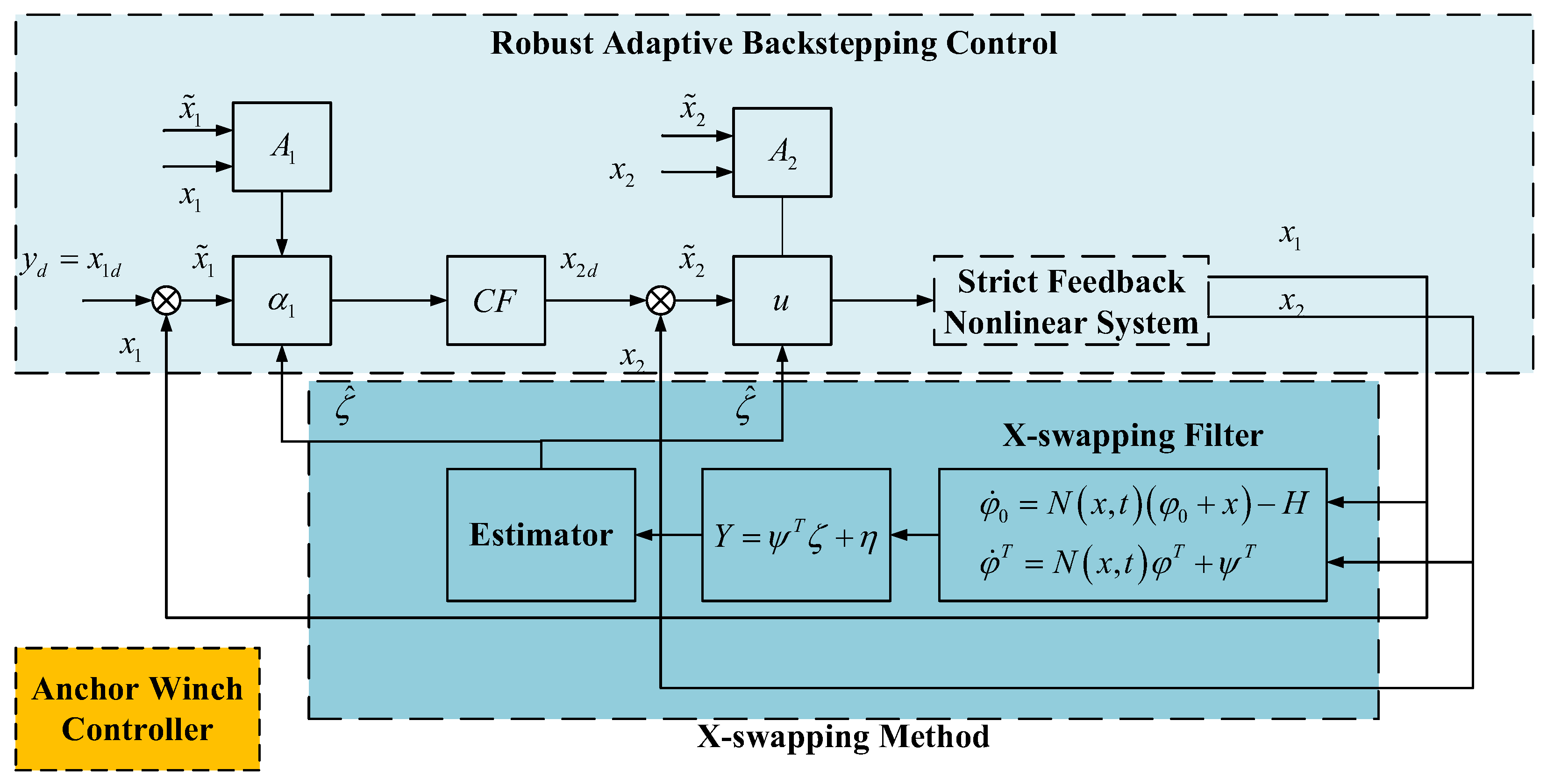
The nonlinear model predictive control method is used in [29] to control the nonlinear system. In contrast, the X−swapping method is used in this work to transform the nonlinear parameters to linear parameters, reducing the calculation costs and control error of the improved LMPC.

(3)

This work converts the cable tension into the desired angular displacement, which is the input of the winch controller. In contrast, the cable tension is set as the control input in [29]. To avoid sudden changes in the remaining cable tension, caused by part cable break-downs, this article only runs the NMPC method in stable state1 (0–15 s).

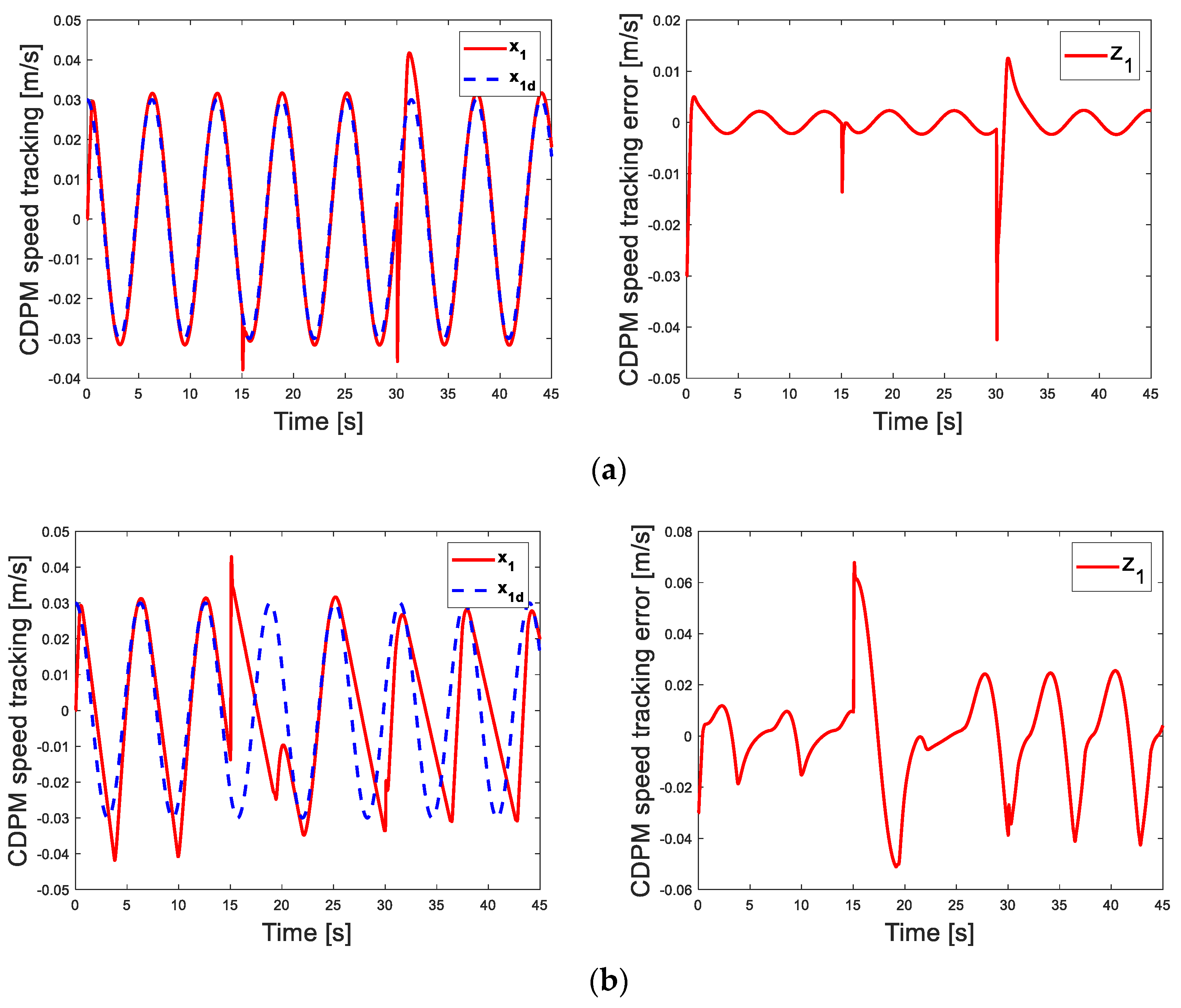
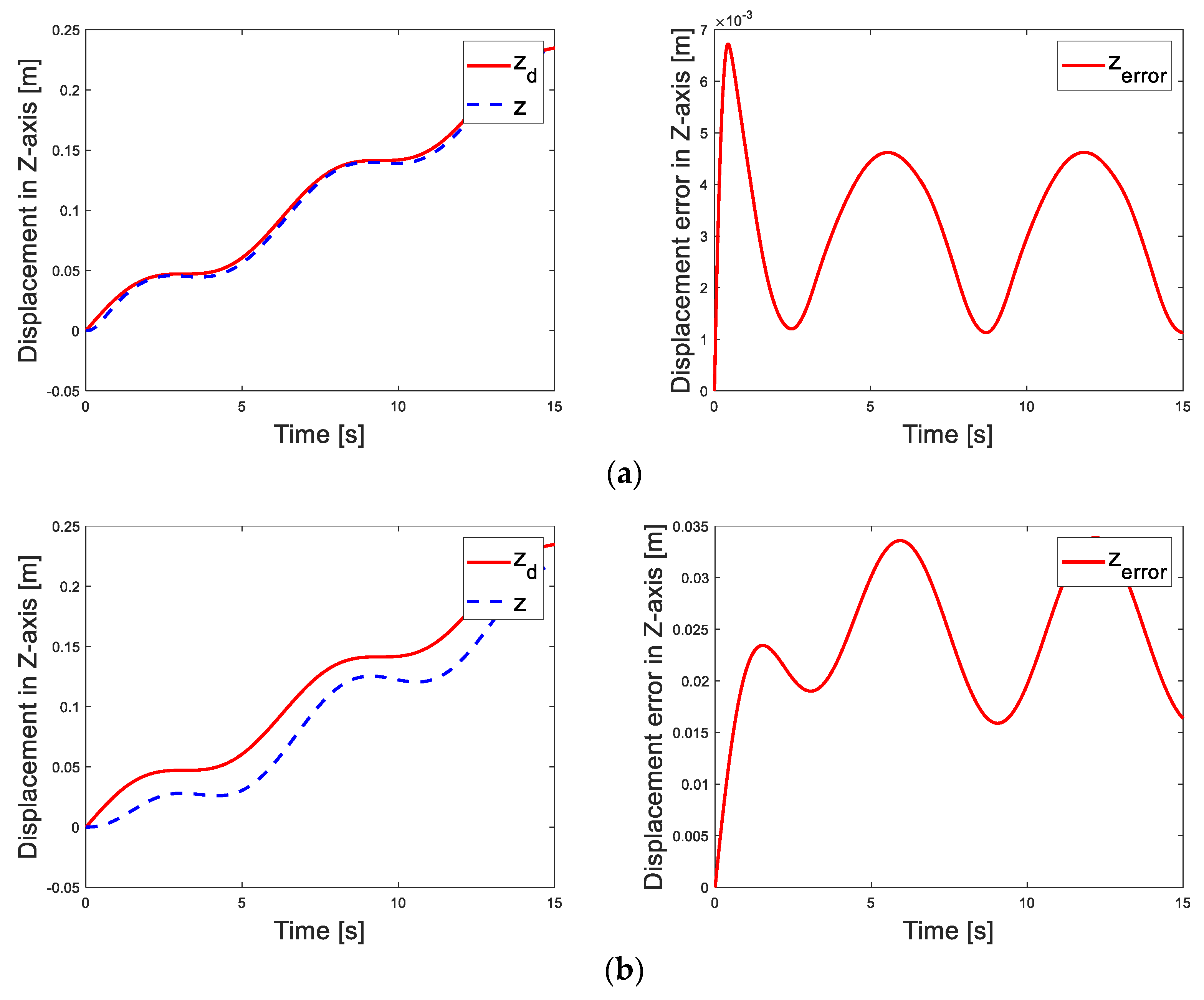
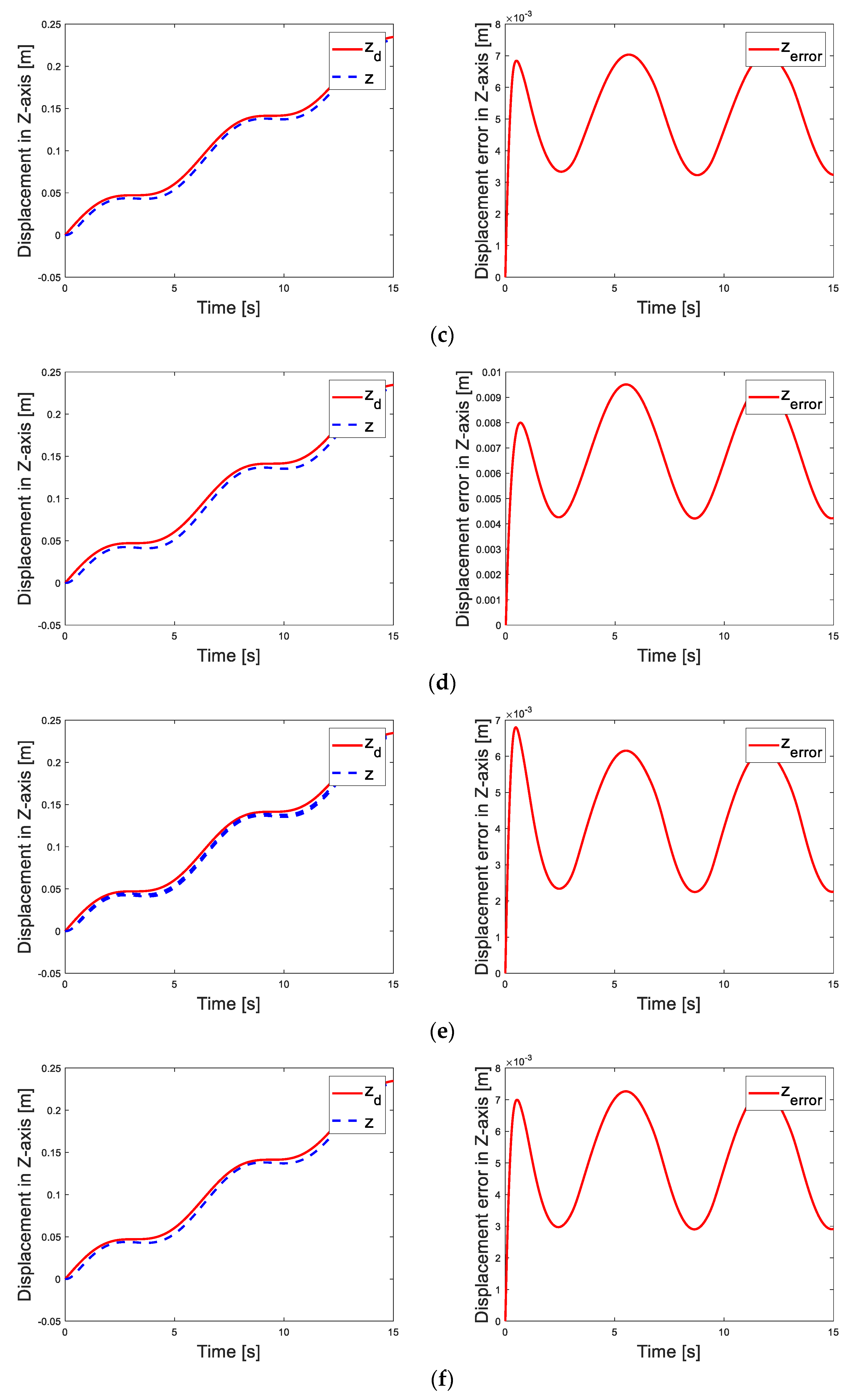
Figure 7a–d represent the speed tracking and tracking error in several situations; the data analyses are summarized in

Table 5. Data analyses of speed-control simulation.

Ideal Speed		${\mathit{x}}_{1\mathit{d}}=0.03\mathbf{cos}\left(\mathit{t}\right)$			${\mathit{x}}_{1\mathit{d}}=0.01\mathbf{cos}\left(\mathit{t}\right)$
Figure 7		(a)	(b)	(e)	(c)	(d)	(f)
Stable state1 (2~15 s)	${\left|z\right|}_{\max }m/s$	0.0022	0.0187	0.0247	$7.41\times {10}^{-4}$	$8.02\times {10}^{-4}$	0.0011
	$\frac{{\left|z\right|}_{\max }}{\left|x_d\right|}\times 100\%$	7.333	62.333	82.333	7.4123	8.02	11.0
Stable state2 (16~28 s)	${\left|z\right|}_{\max }m/s$	0.0023	0.0526	-	$7.77\times {10}^{-4}$	0.0011	-
	$\frac{{\left|z\right|}_{\max }}{\left|x_d\right|}\times 100\%$	7.667	175.333	-	7.7712	11	-
Stable state2 (33~45 s)	${\left|z\right|}_{\max }m/s$	0.0025	0.0425	-	$8.11\times {10}^{-4}$	0.0226	-
	$\frac{{\left|z\right|}_{\max }}{\left|x_d\right|}\times 100\%$	8.3333	141.667	-	8.11	226	-
Average absolute error		0.0023	0.0379	0.0247	$7.7633\times {10}^{-4}$	0.0082	0.0011

. It is easy to find that the entire stage is divided into three parts: all cables intact (0–15 s), one broken cable-stayed cable (15–30 s), and two broken cable-stayed cables (30–45 s). There is significant vibration at 15 s and 30 s, meaning the underwater CDPM experienced a violent upward movement at the cable breakage (the floating speed is negative). According to Table 5, it is clear that when $x_{1d}=0.03\cos \left(t\right)$, the maximum error value (${\left|z\right|}_{\max }$) of the improved LMPC method under stable states (2–15, 16–28, and 33–45 s) are 0.0022, 0.0023, and 0.0025, respectively, which are all smaller than the values (0.0187, 0.0526, and 0.0425) of traditional LMPC. When $x_{2d}=0.01\cos \left(t\right)$, the maximum error of the improved LMPC method is still minor compared to the traditional LMPC ($7.41\times {10}^{-4}<8.02\times {10}^{-4}$, $7.77\times {10}^{-4}<1.1\times {10}^{-3}$, and $8.11\times {10}^{-4}<0.0226$). We can conclude that under the same desired speed and conditions, the improved LMPC with the DMPC method has higher accuracy than traditional MPC methods requiring the manual setting of the lower tension threshold. Compared with Figure 7a,c,e,f, we can also draw a similar conclusion that systems with minimum dynamic tension values have better control accuracy than systems with fixed minimum tension values. Moreover, as shown in Figure 7a,b, we can find that the system with improved LMPC can overcome the impact of cable breakage in a shorter period than the system with the traditional LMPC method. This phenomenon means that the improved LMPC with the DMPC method increases the control accuracy and stability of the system. A similar situation also occurs in Figure 7c,d. These phenomena indicate that the system using the improved LMPC method us more robust than the traditional LMPC method.

Moreover, we find that in Table 5 a, c, and d, the proportion of steady-state error to total amplitude ($\frac{{\left|z\right|}_{\max }}{\left|x_d\right|}\times 100\%$) is less than 10%. On the contrary, in Table 5 b, and e, the proportion of steady-state error to total amplitude ($\frac{{\left|z\right|}_{\max }}{\left|x_d\right|}\times 100\%$) far exceeds 10%. And in Table 5 f, the value slightly exceeds 10%. These phenomena mean that the improved LMPC with the DMPC method can better adapt to different speeds and ensure tracking accuracy. Correspondingly, the traditional LMPC met control requirements in $x_{2d}=0.01\cos \left(t\right)$ and failed in $x_{1d}=0.03\cos \left(t\right)$. According to the comparison results between Figure 7a–f, we can conclude that the improved LMPC can meet different motion speeds without manually setting the minimum tension threshold, which means the better adaptability, fewer prior knowledge requirements, and a broader application range.

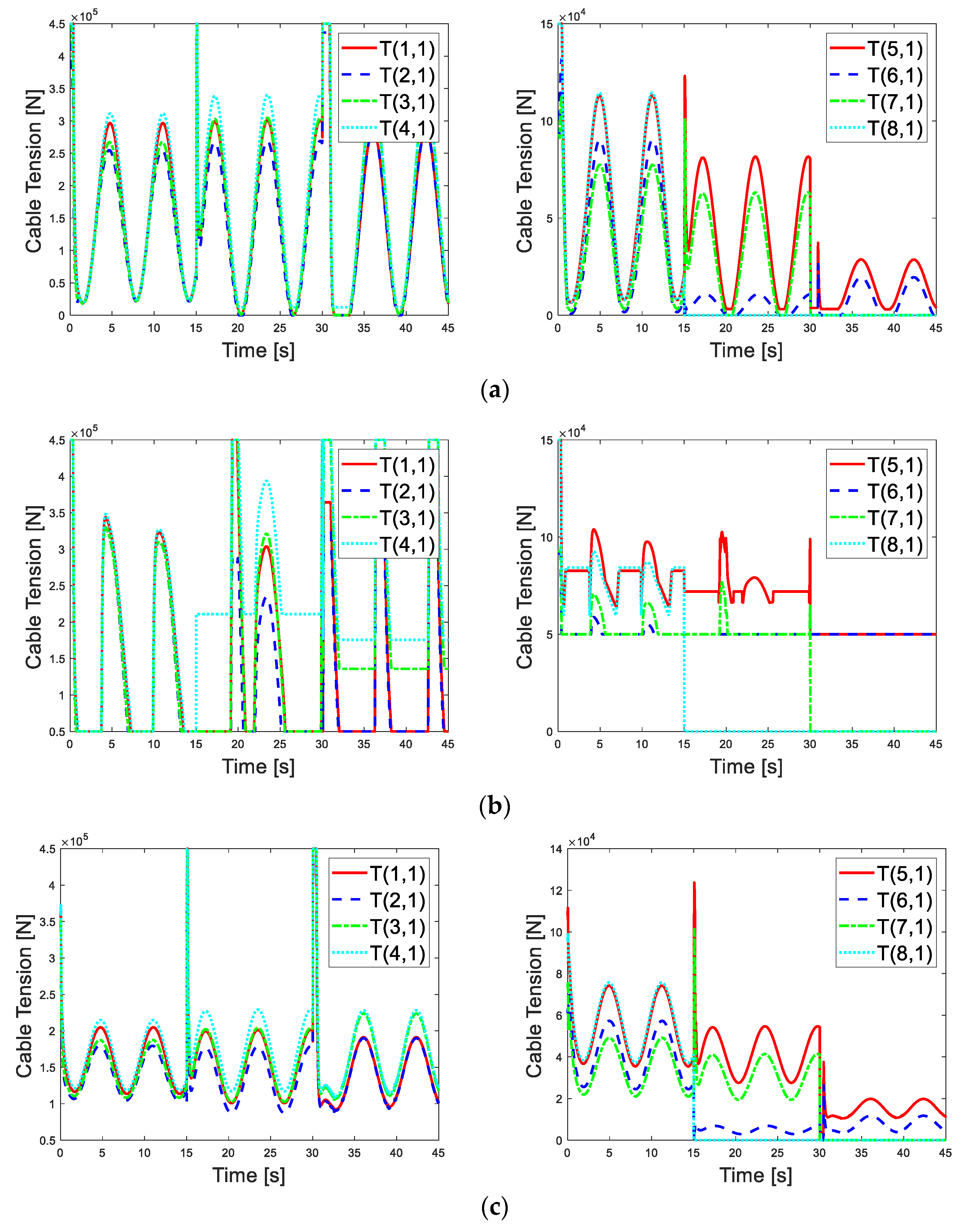
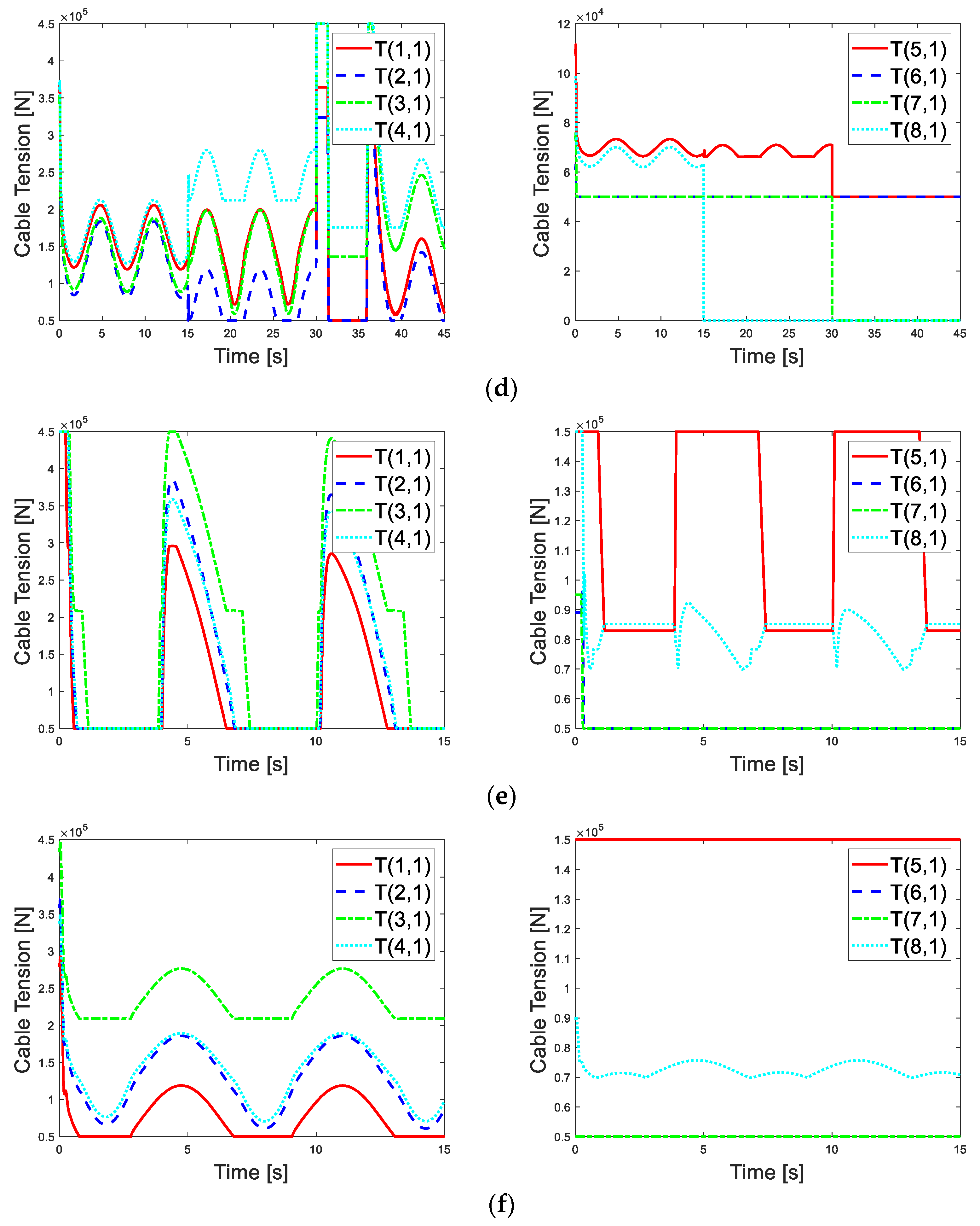
Figure 8a–f represents the tension distribution under different CDPM speeds and winch cable states. The data analyses are summarized in Table 6, Table 7, Table 8, Table 9, Table 10, Table 11, Table 12 and Table 13. According to Figure 8a–f, we can find that the vertical cable-tension values ($T\left(i,1\right),i=1,2,3,4$) are generally higher than those of the cable-stayed cable ($T\left(i,1\right),i=5,6,7,8$). This result is consistent with experience, and we can regard the vertical cable tension as the main factor causing platform motion. In contrast, the cable-stayed cables are chosen as auxiliary influencing factors of platform motion. By comparing the maximum and minimum cable-tension values under various stable states in Table 6, Table 7, Table 8, Table 9, Table 10, Table 11, Table 12 and Table 13, we can find the following situations:

(1)

In most cases, systems using the improved LMPC method have a maximum cable tension lower than the traditional LMPC method and NMPC under stable conditions. According to [27], the lower maximum tension effectively avoids the impact of excessive cable tension on equipment safety, avoids actuator input saturation, and reduces power cost.

(2)

In most cases, systems using the improved LMPC method have lower minimum cable-tension values under stable conditions than systems with traditional LMPC method and NMPC method. These phenomena represent that the former system provides a bigger workspace for the CDPM in all states. Therefore, we can conclude that the improved LMPC method can provide larger workspace and better adaptability.

(3)

As shown in Table 12 and Table 13, we can find that in most cases, the average fluctuation amplitude of cable tension in the system with the improved LMPC method is smaller than the system with the traditional LMPC method and NMPC method. According to [27], the magnitude of stress changes in the cable affects the fatigue and safety of the cable. Therefore, we can conclude that the improved LMPC method has smaller tension amplitude variation, minor cable fatigue, and better equipment safety than the traditional LMPC method and NMPC method.

(4)

As shown in Figure 8a–d, we can find that the improved LMPC method with DMPC can recover from the extreme tension value (upper or lower tension limit) to the usual tension range in a shorter time, which significantly reduces the possible elastic deformation, performance degradation, and cable-sliding phenomenon of the cable under extreme tension.

(5)

As shown in Figure 8a–d and Table 6, Table 7, Table 8, Table 9, Table 10, Table 11, Table 12 and Table 13, we can observe that the cable tension is relatively low at times (in stages 2 and 3 of cable states, part cable breakage). Therefore, the cable slipping caused by low cable tension may affect the motion control accuracy of the platform.

Figure 8. (a) Distribution of cable tension ($F_i=T\left(i,1\right),i=1,2,\dots ,8$) under cosine motion ($x_{1d}=0.03\cos \left(t\right)$) based on the improved LMPC method. (b) Distribution of cable tension ($F_i=T\left(i,1\right),i=1,2,\dots ,8$) under cosine motion ($x_{1d}=0.03\cos \left(t\right)$) based on compared traditional LMPC. (c) Distribution of cable tension ($F_i=T\left(i,1\right),i=1,2,\dots ,8$) under cosine motion ($x_{2d}=0.01\cos \left(t\right)$) based on the improved LMPC method. (d) Distribution of cable tension ($F_i=T\left(i,1\right),i=1,2,\dots ,8$) under cosine motion ($x_{2d}=0.01\cos \left(t\right)$) based on compared traditional LMPC. (e) Distribution of cable tension ($F_i=T\left(i,1\right),i=1,2,\dots ,8$) under cosine motion ($x_{1d}=0.03\cos \left(t\right)$) based on compared NMPC with fixed tension thresholds. (f) Distribution of cable tension ($F_i=T\left(i,1\right),i=1,2,\dots ,8$) under cosine motion ($x_{2d}=0.01\cos \left(t\right)$) based on compared NMPC with fixed tension thresholds.

Figure 8. (a) Distribution of cable tension ($F_i=T\left(i,1\right),i=1,2,\dots ,8$) under cosine motion ($x_{1d}=0.03\cos \left(t\right)$) based on the improved LMPC method. (b) Distribution of cable tension ($F_i=T\left(i,1\right),i=1,2,\dots ,8$) under cosine motion ($x_{1d}=0.03\cos \left(t\right)$) based on compared traditional LMPC. (c) Distribution of cable tension ($F_i=T\left(i,1\right),i=1,2,\dots ,8$) under cosine motion ($x_{2d}=0.01\cos \left(t\right)$) based on the improved LMPC method. (d) Distribution of cable tension ($F_i=T\left(i,1\right),i=1,2,\dots ,8$) under cosine motion ($x_{2d}=0.01\cos \left(t\right)$) based on compared traditional LMPC. (e) Distribution of cable tension ($F_i=T\left(i,1\right),i=1,2,\dots ,8$) under cosine motion ($x_{1d}=0.03\cos \left(t\right)$) based on compared NMPC with fixed tension thresholds. (f) Distribution of cable tension ($F_i=T\left(i,1\right),i=1,2,\dots ,8$) under cosine motion ($x_{2d}=0.01\cos \left(t\right)$) based on compared NMPC with fixed tension thresholds.

Table 6. Data analyses of cable-tension distribution.

Figure 8		(a)				(a)
$\mathbf{Unit}:1\times {10}^5$ N		$\mathit{T}\left(1,1\right)$	$\mathit{T}\left(2,1\right)$	$\mathit{T}\left(3,1\right)$	$\mathit{T}\left(4,1\right)$	$\mathit{T}\left(5,1\right)$	$\mathit{T}\left(6,1\right)$	$\mathit{T}\left(7,1\right)$	$\mathit{T}\left(8,1\right)$
Stable state1 (2~15 s)	Maximum tension	2.9652	2.5480	2.6718	3.1164	1.1316	0.9024	0.7743	1.1448
	Minimum tension	0.23623	0.2144	0.2211	0.2453	0.0785	0.0159	0.0335	0.0793
	Tension amplitude	2.7289	2.3336	2.4507	2.8710	1.0531	0.8865	0.7408	1.0655
Stable state2 (16~28 s)	Maximum tension	3.0113	2.6904	3.0464	3.4023	0.8161	0.1096	0.6328	0
	Minimum tension	0.0109	0.0011	0.0101	0.1235	0.0315	0.0012	0.0013	0
	Tension amplitude	3.0004	2.6893	3.0362	3.2788	0.7846	0.1084	0.6315	0
Stable state3 (33~45 s)	Maximum tension	2.8573	2.8485	3.3497	3.4044	0.2871	0.1976	0	0
	Minimum tension	0.0004	0.0016	0.0011	0.1237	0.0301	0.0021	0	0
	Tension amplitude	2.8569	2.8469	3.3486	3.2807	0.2570	0.1955	0	0
Average tension amplitude		2.8621	2.6233	2.9452	3.1435	0.6982	0.3968	0.4574	0.3552

Table 6. Data analyses of cable-tension distribution.

Figure 8		(a)				(a)
$\mathbf{Unit}:1\times {10}^5$ N		$\mathit{T}\left(1,1\right)$	$\mathit{T}\left(2,1\right)$	$\mathit{T}\left(3,1\right)$	$\mathit{T}\left(4,1\right)$	$\mathit{T}\left(5,1\right)$	$\mathit{T}\left(6,1\right)$	$\mathit{T}\left(7,1\right)$	$\mathit{T}\left(8,1\right)$
Stable state1 (2~15 s)	Maximum tension	2.9652	2.5480	2.6718	3.1164	1.1316	0.9024	0.7743	1.1448
	Minimum tension	0.23623	0.2144	0.2211	0.2453	0.0785	0.0159	0.0335	0.0793
	Tension amplitude	2.7289	2.3336	2.4507	2.8710	1.0531	0.8865	0.7408	1.0655
Stable state2 (16~28 s)	Maximum tension	3.0113	2.6904	3.0464	3.4023	0.8161	0.1096	0.6328	0
	Minimum tension	0.0109	0.0011	0.0101	0.1235	0.0315	0.0012	0.0013	0
	Tension amplitude	3.0004	2.6893	3.0362	3.2788	0.7846	0.1084	0.6315	0
Stable state3 (33~45 s)	Maximum tension	2.8573	2.8485	3.3497	3.4044	0.2871	0.1976	0	0
	Minimum tension	0.0004	0.0016	0.0011	0.1237	0.0301	0.0021	0	0
	Tension amplitude	2.8569	2.8469	3.3486	3.2807	0.2570	0.1955	0	0
Average tension amplitude		2.8621	2.6233	2.9452	3.1435	0.6982	0.3968	0.4574	0.3552

Table 7. Data analyses of cable-tension distribution.

Figure 8		(b)				(b)
$\mathbf{Unit}:1\times {10}^5$ N		$\mathit{T}\left(1,1\right)$	$\mathit{T}\left(2,1\right)$	$\mathit{T}\left(3,1\right)$	$\mathit{T}\left(4,1\right)$	$\mathit{T}\left(5,1\right)$	$\mathit{T}\left(6,1\right)$	$\mathit{T}\left(7,1\right)$	$\mathit{T}\left(8,1\right)$
Stable state1 (2~15 s)	Maximum tension	3.4400	3.2961	3.2997	3.4826	1.0394	0.5880	0.7057	0.9265
	Minimum tension	0.5	0.5	0.5	0.5	0.6426	0.5	0.5	0.5958
	Tension amplitude	2.9400	2.7961	2.7997	2.9826	0.3968	0.08797	0.2057	0.3307
Stable state2 (16~28 s)	Maximum tension	4.5	2.8783	4.5	4.5	1.0257	0.5	0.7679	0
	Minimum tension	0.5	0.5	0.5	2.1089	0.6626	0.5	0.5	0
	Tension amplitude	4.0000	2.3783	4.0000	2.3911	0.3631	0	0.2679	0
Stable state3 (33~45 s)	Maximum tension	3.6428	3.2375	4.5	4.5	0.5	0.5	0	0
	Minimum tension	0.5	0.5	1.3585	1.7556	0.5	0.5	0	0
	Tension amplitude	3.1428	2.7375	3.1415	2.7444	0	0	0	0
Average tension amplitude		3.3609	2.6373	3.3137	2.7060	0.2533	0.0293	0.1579	0.1102

Table 7. Data analyses of cable-tension distribution.

Figure 8		(b)				(b)
$\mathbf{Unit}:1\times {10}^5$ N		$\mathit{T}\left(1,1\right)$	$\mathit{T}\left(2,1\right)$	$\mathit{T}\left(3,1\right)$	$\mathit{T}\left(4,1\right)$	$\mathit{T}\left(5,1\right)$	$\mathit{T}\left(6,1\right)$	$\mathit{T}\left(7,1\right)$	$\mathit{T}\left(8,1\right)$
Stable state1 (2~15 s)	Maximum tension	3.4400	3.2961	3.2997	3.4826	1.0394	0.5880	0.7057	0.9265
	Minimum tension	0.5	0.5	0.5	0.5	0.6426	0.5	0.5	0.5958
	Tension amplitude	2.9400	2.7961	2.7997	2.9826	0.3968	0.08797	0.2057	0.3307
Stable state2 (16~28 s)	Maximum tension	4.5	2.8783	4.5	4.5	1.0257	0.5	0.7679	0
	Minimum tension	0.5	0.5	0.5	2.1089	0.6626	0.5	0.5	0
	Tension amplitude	4.0000	2.3783	4.0000	2.3911	0.3631	0	0.2679	0
Stable state3 (33~45 s)	Maximum tension	3.6428	3.2375	4.5	4.5	0.5	0.5	0	0
	Minimum tension	0.5	0.5	1.3585	1.7556	0.5	0.5	0	0
	Tension amplitude	3.1428	2.7375	3.1415	2.7444	0	0	0	0
Average tension amplitude		3.3609	2.6373	3.3137	2.7060	0.2533	0.0293	0.1579	0.1102

Table 8. Data analyses of cable-tension distribution.

Figure 8		(c)				(c)
$\mathbf{Unit}:1\times {10}^5$ N		$\mathit{T}\left(1,1\right)$	$\mathit{T}\left(2,1\right)$	$\mathit{T}\left(3,1\right)$	$\mathit{T}\left(4,1\right)$	$\mathit{T}\left(5,1\right)$	$\mathit{T}\left(6,1\right)$	$\mathit{T}\left(7,1\right)$	$\mathit{T}\left(8,1\right)$
Stable state1 (2~15 s)	Maximum tension	2.0483	1.7951	1.8754	2.1479	0.7422	0.5729	0.4915	0.7575
	Minimum tension	1.1353	1.0457	1.0826	1.1836	0.3544	0.2448	0.2099	0.3718
	Tension amplitude	0.9129	0.7494	0.7928	0.9643	0.3878	0.3281	0.2816	0.3857
Stable state2 (16~28 s)	Maximum tension	2.0136	1.7847	2.0397	2.2911	0.5468	0.0688	0.4136	0
	Minimum tension	1.0087	0.8731	1.0259	1.1724	0.2756	0.0293	0.1941	0
	Tension amplitude	1.0050	0.9115	1.0138	1.1188	0.2712	0.0395	0.2195	0
Stable state3 (33~45 s)	Maximum tension	1.9132	1.9003	2.2384	2.2819	0.1985	0.1176	0	0
	Minimum tension	0.9054	0.8883	1.0519	1.0831	0.1035	0.0345	0	0
	Tension amplitude	1.0078	1.0120	1.1865	1.1988	0.0950	0.0831	0	0
Average tension amplitude		0.9752	0.8910	0.9977	1.094	0.2513	0.1502	0.1670	0.1286

Table 8. Data analyses of cable-tension distribution.

Figure 8		(c)				(c)
$\mathbf{Unit}:1\times {10}^5$ N		$\mathit{T}\left(1,1\right)$	$\mathit{T}\left(2,1\right)$	$\mathit{T}\left(3,1\right)$	$\mathit{T}\left(4,1\right)$	$\mathit{T}\left(5,1\right)$	$\mathit{T}\left(6,1\right)$	$\mathit{T}\left(7,1\right)$	$\mathit{T}\left(8,1\right)$
Stable state1 (2~15 s)	Maximum tension	2.0483	1.7951	1.8754	2.1479	0.7422	0.5729	0.4915	0.7575
	Minimum tension	1.1353	1.0457	1.0826	1.1836	0.3544	0.2448	0.2099	0.3718
	Tension amplitude	0.9129	0.7494	0.7928	0.9643	0.3878	0.3281	0.2816	0.3857
Stable state2 (16~28 s)	Maximum tension	2.0136	1.7847	2.0397	2.2911	0.5468	0.0688	0.4136	0
	Minimum tension	1.0087	0.8731	1.0259	1.1724	0.2756	0.0293	0.1941	0
	Tension amplitude	1.0050	0.9115	1.0138	1.1188	0.2712	0.0395	0.2195	0
Stable state3 (33~45 s)	Maximum tension	1.9132	1.9003	2.2384	2.2819	0.1985	0.1176	0	0
	Minimum tension	0.9054	0.8883	1.0519	1.0831	0.1035	0.0345	0	0
	Tension amplitude	1.0078	1.0120	1.1865	1.1988	0.0950	0.0831	0	0
Average tension amplitude		0.9752	0.8910	0.9977	1.094	0.2513	0.1502	0.1670	0.1286

Table 9. Data analyses of cable-tension distribution.

Figure 8		(d)				(d)
$\mathbf{Unit}:1\times {10}^5$ N		$\mathit{T}\left(1,1\right)$	$\mathit{T}\left(2,1\right)$	$\mathit{T}\left(3,1\right)$	$\mathit{T}\left(4,1\right)$	$\mathit{T}\left(5,1\right)$	$\mathit{T}\left(6,1\right)$	$\mathit{T}\left(7,1\right)$	$\mathit{T}\left(8,1\right)$
Stable state1 (2~15 s)	Maximum tension	2.0566	1.8328	1.8837	2.1268	7.3364	5	5	7.0068
	Minimum tension	1.1908	0.8121	0.8883	1.2701	6.6452	5	5	6.2017
	Tension amplitude	0.8658	1.0207	0.9953	0.8567	0.6912	0	0	0.8051
Stable state2 (16~28 s)	Maximum tension	1.9968	1.1931	1.9873	2.8026	7.1008	5	5	0
	Minimum tension	0.7189	0.5	0.5934	2.1186	6.6131	5	5	0
	Tension amplitude	1.2779	0.6931	1.3939	0.6840	0.4877	0	0	0
Stable state3 (33~45 s)	Maximum tension	3.6429	3.2375	4.5	4.5	5	5	0	0
	Minimum tension	0.5	0.5	1.3587	1.7556	5	5	0	0
	Tension amplitude	3.1429	2.7375	3.1413	2.7444	0	0	0	0
Average tension amplitude		1.7622	1.4837	1.8435	1.4283	0.3927	0	0	0.2684

Table 9. Data analyses of cable-tension distribution.

Figure 8		(d)				(d)
$\mathbf{Unit}:1\times {10}^5$ N		$\mathit{T}\left(1,1\right)$	$\mathit{T}\left(2,1\right)$	$\mathit{T}\left(3,1\right)$	$\mathit{T}\left(4,1\right)$	$\mathit{T}\left(5,1\right)$	$\mathit{T}\left(6,1\right)$	$\mathit{T}\left(7,1\right)$	$\mathit{T}\left(8,1\right)$
Stable state1 (2~15 s)	Maximum tension	2.0566	1.8328	1.8837	2.1268	7.3364	5	5	7.0068
	Minimum tension	1.1908	0.8121	0.8883	1.2701	6.6452	5	5	6.2017
	Tension amplitude	0.8658	1.0207	0.9953	0.8567	0.6912	0	0	0.8051
Stable state2 (16~28 s)	Maximum tension	1.9968	1.1931	1.9873	2.8026	7.1008	5	5	0
	Minimum tension	0.7189	0.5	0.5934	2.1186	6.6131	5	5	0
	Tension amplitude	1.2779	0.6931	1.3939	0.6840	0.4877	0	0	0
Stable state3 (33~45 s)	Maximum tension	3.6429	3.2375	4.5	4.5	5	5	0	0
	Minimum tension	0.5	0.5	1.3587	1.7556	5	5	0	0
	Tension amplitude	3.1429	2.7375	3.1413	2.7444	0	0	0	0
Average tension amplitude		1.7622	1.4837	1.8435	1.4283	0.3927	0	0	0.2684

Table 10. Data analyses of cable-tension distribution.

Figure 8		(e)				(e)
$\mathbf{Unit}:1\times {10}^5$ N		$\mathit{T}\left(1,1\right)$	$\mathit{T}\left(2,1\right)$	$\mathit{T}\left(3,1\right)$	$\mathit{T}\left(4,1\right)$	$\mathit{T}\left(5,1\right)$	$\mathit{T}\left(6,1\right)$	$\mathit{T}\left(7,1\right)$	$\mathit{T}\left(8,1\right)$
Stable state1 (2~15 s)	Maximum tension	2.9582	3.8497	4.5	3.5904	1.5	0.5	0.5	0.9241
	Minimum tension	0.5	0.5	0.5	0.5	0.8287	0.5	0.5	0.6982
	Tension amplitude	2.4582	3.3497	4.0	3.0904	0.6713	0	0	0.2259

Table 10. Data analyses of cable-tension distribution.

Figure 8		(e)				(e)
$\mathbf{Unit}:1\times {10}^5$ N		$\mathit{T}\left(1,1\right)$	$\mathit{T}\left(2,1\right)$	$\mathit{T}\left(3,1\right)$	$\mathit{T}\left(4,1\right)$	$\mathit{T}\left(5,1\right)$	$\mathit{T}\left(6,1\right)$	$\mathit{T}\left(7,1\right)$	$\mathit{T}\left(8,1\right)$
Stable state1 (2~15 s)	Maximum tension	2.9582	3.8497	4.5	3.5904	1.5	0.5	0.5	0.9241
	Minimum tension	0.5	0.5	0.5	0.5	0.8287	0.5	0.5	0.6982
	Tension amplitude	2.4582	3.3497	4.0	3.0904	0.6713	0	0	0.2259

Table 11. Data analyses of cable-tension distribution.

Figure 8		(f)				(f)
$\mathbf{Unit}:1\times {10}^5$ N		$\mathit{T}\left(1,1\right)$	$\mathit{T}\left(2,1\right)$	$\mathit{T}\left(3,1\right)$	$\mathit{T}\left(4,1\right)$	$\mathit{T}\left(5,1\right)$	$\mathit{T}\left(6,1\right)$	$\mathit{T}\left(7,1\right)$	$\mathit{T}\left(8,1\right)$
Stable state1 (2~15 s)	Maximum tension	1.1885	1.8590	2.7655	1.8938	1.5	1.5	0.5	0.7571
	Minimum tension	0.5	0.6101	2.0877	0.7071	1.5	1.5	0.5	0.6981
	Tension amplitude	0.6886	1.2489	0.6777	1.1867	0	0	0	0.0590

Table 11. Data analyses of cable-tension distribution.

Figure 8		(f)				(f)
$\mathbf{Unit}:1\times {10}^5$ N		$\mathit{T}\left(1,1\right)$	$\mathit{T}\left(2,1\right)$	$\mathit{T}\left(3,1\right)$	$\mathit{T}\left(4,1\right)$	$\mathit{T}\left(5,1\right)$	$\mathit{T}\left(6,1\right)$	$\mathit{T}\left(7,1\right)$	$\mathit{T}\left(8,1\right)$
Stable state1 (2~15 s)	Maximum tension	1.1885	1.8590	2.7655	1.8938	1.5	1.5	0.5	0.7571
	Minimum tension	0.5	0.6101	2.0877	0.7071	1.5	1.5	0.5	0.6981
	Tension amplitude	0.6886	1.2489	0.6777	1.1867	0	0	0	0.0590

Table 12. Data analyses of average cable-tension amplitude.

Figure 8	(a)	(b)	Relationship between (a) and (b)	(e)	Relationship between (a) and (e)
$T\left(1,1\right)$$(\times {10}^5$ N)	2.8621	3.3609	<	2.9582	<
$T\left(2,1\right)$$(\times {10}^5$ N)	2.6233	2.6373	<	3.8497	<
$T\left(3,1\right)$$(\times {10}^5$ N)	2.9452	3.3137	<	4.5	<
$T\left(4,1\right)$$(\times {10}^5$ N)	3.1435	2.7060	>	3.5904	<

Table 12. Data analyses of average cable-tension amplitude.

Figure 8	(a)	(b)	Relationship between (a) and (b)	(e)	Relationship between (a) and (e)
$T\left(1,1\right)$$(\times {10}^5$ N)	2.8621	3.3609	<	2.9582	<
$T\left(2,1\right)$$(\times {10}^5$ N)	2.6233	2.6373	<	3.8497	<
$T\left(3,1\right)$$(\times {10}^5$ N)	2.9452	3.3137	<	4.5	<
$T\left(4,1\right)$$(\times {10}^5$ N)	3.1435	2.7060	>	3.5904	<

Table 13. Data analyses of average cable-tension amplitude.

Figure 8	(c)	(d)	Relationship between (c) and (d)	(f)	Relationship between (c) and (f)
$T\left(1,1\right)$$(\times {10}^5$ N)	0.9752	1.7622	<	0.6886	>
$T\left(2,1\right)$$(\times {10}^5$ N)	0.8901	1.4837	<	1.2489	<
$T\left(3,1\right)$$(\times {10}^5$ N)	0.9977	1.8435	<	0.6777	>
$T\left(4,1\right)$$(\times {10}^5$ N)	1.0940	1.4283	<	1.1867	<

Table 13. Data analyses of average cable-tension amplitude.

Figure 8	(c)	(d)	Relationship between (c) and (d)	(f)	Relationship between (c) and (f)
$T\left(1,1\right)$$(\times {10}^5$ N)	0.9752	1.7622	<	0.6886	>
$T\left(2,1\right)$$(\times {10}^5$ N)	0.8901	1.4837	<	1.2489	<
$T\left(3,1\right)$$(\times {10}^5$ N)	0.9977	1.8435	<	0.6777	>
$T\left(4,1\right)$$(\times {10}^5$ N)	1.0940	1.4283	<	1.1867	<

Remark 5. 

There are two explanations for a tension amplitude value of zero: (1) the cable-tension value is the lower threshold of cable tension, and the maximum tension is equal to the minimum tension or (2) the cable is broken, and the tension value is zero.

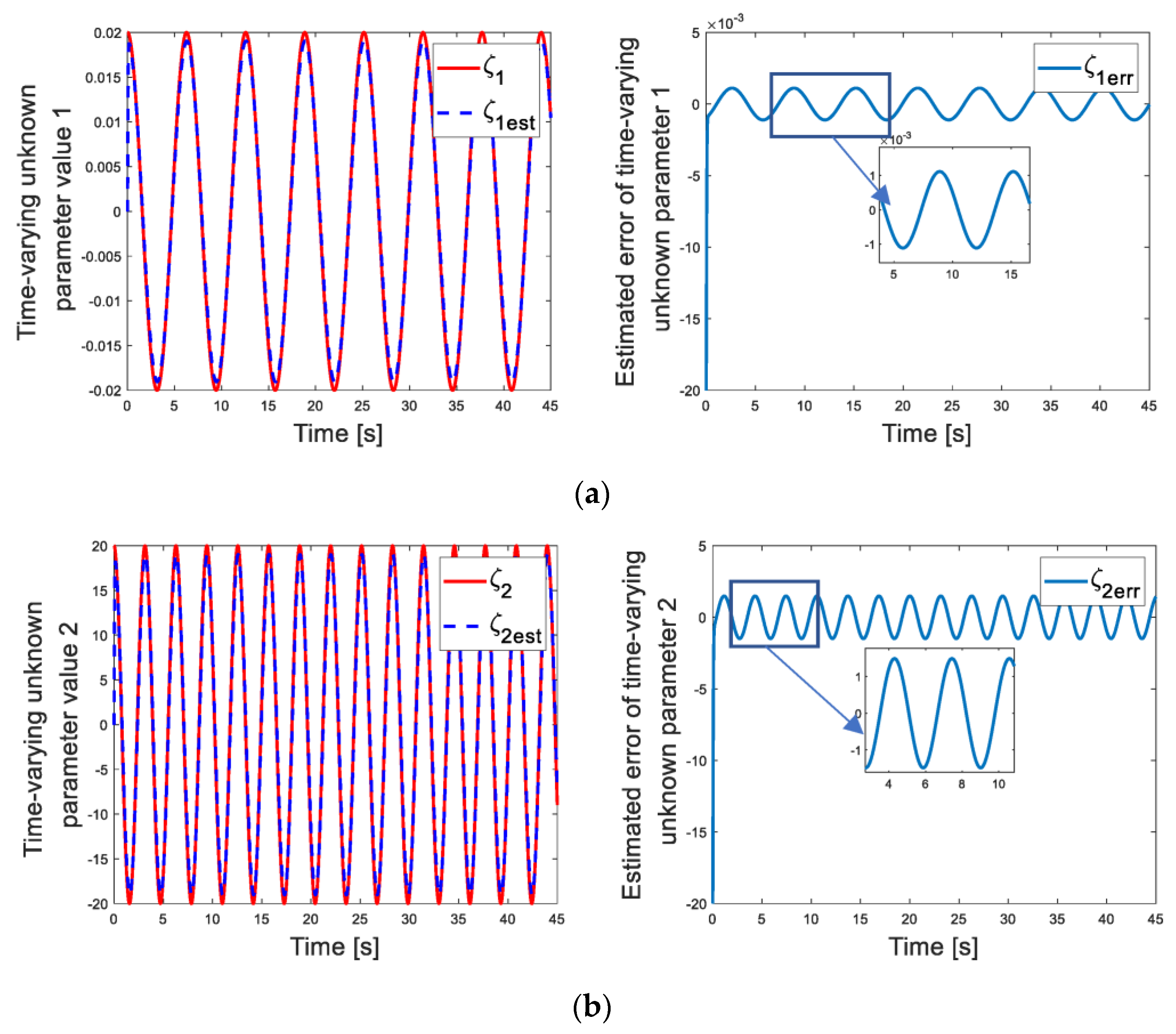
The time−varying unknown parameters, estimated value, and estimated error curves are shown in Figure 9. When the tracking curve is stable, we can observe that the maximum absolute estimation error and error ratios of the time−varying unknown parameter ${\zeta }_1$ are 0.0011 and 5.5%, respectively. The maximum absolute estimation error and error ratios of the time−varying unknown parameter ${\zeta }_2$ are 1.4888 and 7.44%. We can find that the control system with the DMPC method has higher estimation accuracy for time−varying unknown parameters ${\zeta }_1$ and ${\zeta }_2$. According to Equation (38), ${\lambda }_1$ and ${\lambda }_2$ are functions of ${\zeta }_1$ and ${\zeta }_2$. Therefore, the X−swapping method effectively realizes the linearization and estimation of nonlinear uncertain parameters. Considering that there are far more nonlinear systems than linear systems in the virtual environment, the X−swapping method effectively expands the application range of the linear-mode predictive control method, avoids the complexity of the nonlinear-mode predictive control method, and reduces the amount of calculation.

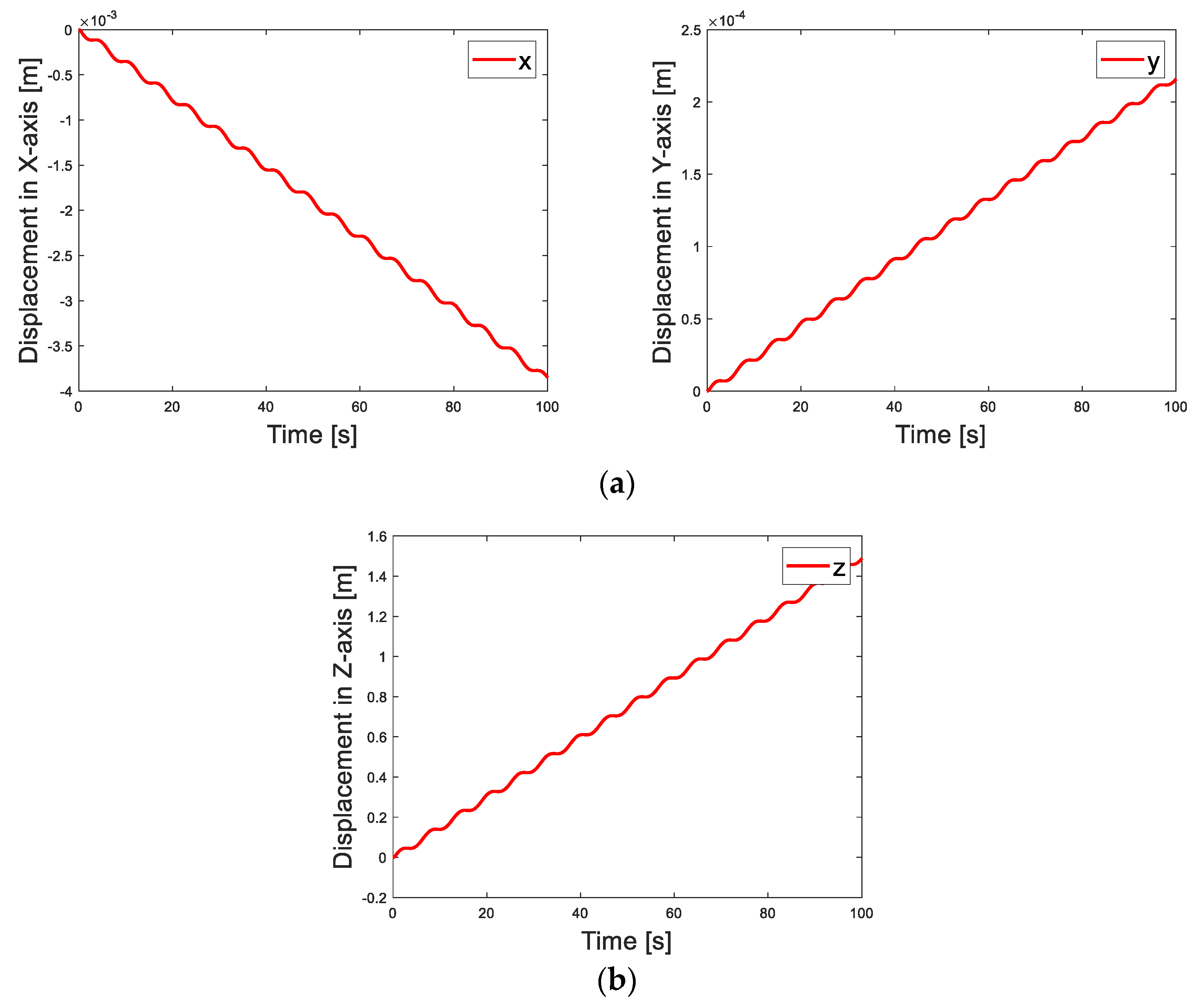
Figure 10 expresses the displacement of CDPM in the $X$, $Y$, and $Z$-axis directions, respectively. It is easy to find that the displacement value of CDPM in the horizontal ($4\times {10}^{-3}$ m and $2.5\times {10}^{-4}$ m) direction is far less than the vertical displacement (1.45 m) of CDPM. Compared to the working depth (60 m) and vertical displacement (1.45 m) of CDPM, the horizontal displacements are so small that the impact on the angle between cables and CDPM is ignored. Therefore, we can conclude that the improved LMPC method with dynamic minimum tension control can effectively avoid the impact of horizontal impact force and suppress the horizontal displacement of CDPM.

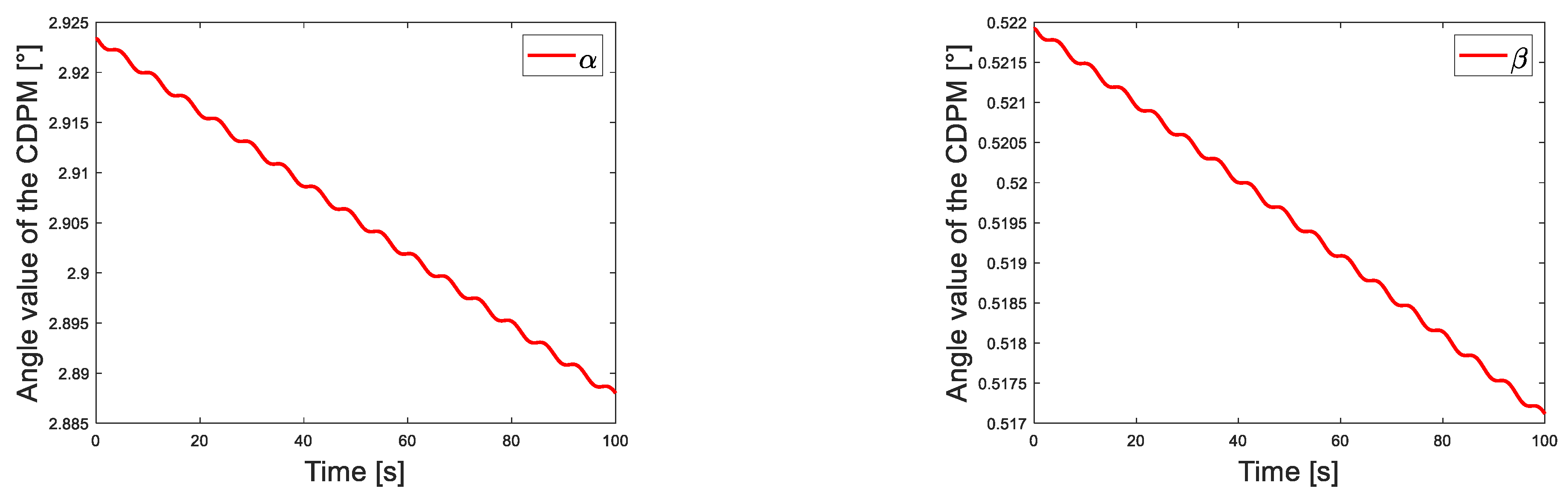
As shown in Figure 11, the angle value of CDPM is $2{.8880}^{\circ }\le \alpha \le 2{.9234}^{\circ }$ and $0.4701\le \beta \le 0.4745$ during the simulation, which meets the requirement ($\left|\alpha \right|\le 3^{\circ },\left|\beta \right|\le {0.5}^{\circ }$ ). Furthermore, combined with the amplitude and duration of motion in Figure 10b, we can observe that CDPM maintains a slow and stable horizontal stabilization trend, and the angle change values are ${0.0354}^{\circ }$ and ${0.0044}^{\circ }$. Based on the trend changes in platform attitude angles, as the platform continues to descend, its original attitude will slowly but continuously adjust to a horizontal state. The platform’s attitude meets the control requirements and constantly improves throughout the moving process. This phenomenon proves the effectiveness of the synchronization control strategy and improved LMPC method used in this paper.

Four primary sources of parameters that affect the CDPM’s motion are mentioned in this article: $k_{s,\inf }$, $k_{v,\inf }$, and $K_{cf}$ in DMPC $K_Y$ and $K_U$ in the LMPC design; control parameters of the X−swapping method; and winch control. The previous text introduced the reasons for selecting control parameters except for $K_Y$ and $K_U$. The following is the impact of the value of $K_Y$ and $K_U$ on the control system.

According to [19], the control effect of the LMPC method is affected by the value of $K_Y$ and $K_U$ in Equation (29). There are six simulation experiments, and the experiment results are shown in Figure 12 and

Table 14. Motion-tracking data of CDPM with variation $K_Y$ and constant $K_U$.

	Figure 12	$${\mathit{K}}_{\mathit{U}}$$	Max Tracking Error (m)
$K_Y$	$(\mathrm{a})\left[\begin{array}{l}8.1\times {10}^{11}{I}_{3\times 3}8.1\times {10}^{11}{I}_{3\times 3}\\ 8.1\times {10}^{11}{I}_{3\times 3}6.3\times {10}^{11}{I}_{3\times 3}\end{array}\right]$	$9\times {10}^{-6}{I}_{8\times 8}$	0.0067
	$(\mathrm{b})\left[\begin{array}{l}1\times {10}^{11}{I}_{3\times 3}1\times {10}^{11}{I}_{3\times 3}\\ 1\times {10}^{11}{I}_{3\times 3}1\times {10}^{11}{I}_{3\times 3}\end{array}\right]$	$9\times {10}^{-6}{I}_{8\times 8}$	0.0339
	$(\mathrm{c})\left[\begin{array}{l}5\times {10}^{11}{I}_{3\times 3}5\times {10}^{11}{I}_{3\times 3}\\ 5\times {10}^{11}{I}_{3\times 3}5\times {10}^{11}{I}_{3\times 3}\end{array}\right]$	$9\times {10}^{-6}{I}_{8\times 8}$	0.0070

and

Table 15. Motion-tracking data of CDPM with constant $K_Y$ and variation $K_U$.

	Figure 12	$${\mathit{K}}_{\mathit{Y}}$$	Max Tracking Error (m)
$K_U$	$(\mathrm{a})9\times {10}^{-6}{I}_{8\times 8}$	$\left[\begin{array}{l}8.1\times {10}^{11}{I}_{3\times 3}8.1\times {10}^{11}{I}_{3\times 3}\\ 8.1\times {10}^{11}{I}_{3\times 3}6.3\times {10}^{11}{I}_{3\times 3}\end{array}\right]$	0.0067
	$(\mathrm{d})20\times {10}^{-6}{I}_{8\times 8}$	$\left[\begin{array}{l}8.1\times {10}^{11}{I}_{3\times 3}8.1\times {10}^{11}{I}_{3\times 3}\\ 8.1\times {10}^{11}{I}_{3\times 3}6.3\times {10}^{11}{I}_{3\times 3}\end{array}\right]$	0.0095
	$(\mathrm{e})12.5\times {10}^{-6}{I}_{8\times 8}$	$\left[\begin{array}{l}8.1\times {10}^{11}{I}_{3\times 3}8.1\times {10}^{11}{I}_{3\times 3}\\ 8.1\times {10}^{11}{I}_{3\times 3}6.3\times {10}^{11}{I}_{3\times 3}\end{array}\right]$	0.0068
	$(\mathrm{f})1.5\times {10}^{-5}{I}_{8\times 8}$	$\left[\begin{array}{l}8.1\times {10}^{11}{I}_{3\times 3}8.1\times {10}^{11}{I}_{3\times 3}\\ 8.1\times {10}^{11}{I}_{3\times 3}6.3\times {10}^{11}{I}_{3\times 3}\end{array}\right]$	0.0073

. Due to the same symbolic meaning as in [35], the values of $K_Y$ and $K_U$ are selected based on this reference, and continuous adjustments and attempts are made based on simulation. According to the figures and tables, we can find that when $K_Y=\left[\begin{array}{l}8.1\times {10}^{11}{I}_{3\times 3}8.1\times {10}^{11}{I}_{3\times 3}\\ 8.1\times {10}^{11}{I}_{3\times 3}6.3\times {10}^{11}{I}_{3\times 3}\end{array}\right]$ and $K_U=9\times {10}^{-6}{I}_{8\times 8}$, the maximum tracking error is minor in a series of experiments. So, the larger $K_Y$ and the smaller $K_U$ will lead to smaller tracking error values when $K_Y$ and $K_U$ are chosen within a specific range, while experiments determine the range.

5. Conclusions

This paper addresses the problem of dynamic modeling and control of an underwater CDPM in three states: zero broken cables, one broken cable-stayed cable, and two broken cable-strayed cables. Firstly, a dynamic model of CDPM is proposed. Next, the DMTC method is proposed to adjust the lower threshold of cable tension, which avoids the conflict between the remaining cable tension value and the fixed lower threshold of cable tension after cable breakage. Then, the improved MPC with the DMTC method is used to convert the underwater CDPM posture and motion state to the desired tension value of the winch. Thirdly, the robust adaptive backstepping controller is designed to realize closed-loop control of the winch, which is based on the joint-space method and command filtering. For uncertain nonlinear parameters in the system, the X−swapping method is used to linearize and identify the time−varying nonlinear parameters and avoid the influence of nonlinear factors on the control accuracy. Finally, the simulation experiments verify the correctness and effectiveness of the model and control method. Considering the impact of cable sag, CDPM flexible deformation, and elastic elongation of cables, future use in the ocean may face more significant challenges. Hence, more work should be carried out to improve the performance of controllers.

References

1. Job, J.; Ponnan, R.J.; Chandran, V.J.; Biju, N. Workspace analysis of an underconstrained cable-driven parallel robot with four cables. Constr. Robot. 2022, 6, 109–119. [Google Scholar] [CrossRef]
2. Qian, S.; Bao, K.; Zi, B.; Wang, N. Kinematic Calibration of a Cable-Driven Parallel Robot for 3D Printing. Sensors 2018, 18, 2898. [Google Scholar] [CrossRef] [PubMed] [Green Version]
3. Anas, S.M.; Alam, M. Performance of brick-filled reinforced concrete composite wall strengthened with C-FRP laminate (s) under blast loading. Mater. Today Proc. 2022, 65, 1–11. [Google Scholar] [CrossRef]
4. Xia, Y.; Xu, G.; Xu, K.; Chen, Y.; Xiang, X.; Ji, Z. Dynamics and control of underwater tension leg platform for diving and leveling. Ocean Eng. 2015, 109, 454–478. [Google Scholar] [CrossRef]
5. Pinto, A.M.; Moreira, E.; Lima, J.; Sousa, J.P.; Costa, P. A cable-driven robot for architectural constructions: A visual-guided approach for motion control and path-planning. Auton. Robot. 2017, 41, 1487–1499. [Google Scholar] [CrossRef]
6. Horoub, M.M.; Hassan, M.; Hawwa, M.A. Workspace analysis of a Gough-Stewart type cable marine platform subjected to harmonic water waves. Mech. Mach. Theory 2018, 120, 314–325. [Google Scholar] [CrossRef]
7. Horoub, M.; Hawwa, M. Influence of cables layout on the dynamic workspace of a six-DOF parallel marine manipulator. Mech. Mach. Theory 2018, 129, 191–201. [Google Scholar] [CrossRef]
8. Zi, B.; Wang, N.; Qian, S.; Bao, K. Design, stiffness analysis and experimental study of a cable-driven parallel 3D printer. Mech. Mach. Theory 2019, 132, 207–222. [Google Scholar] [CrossRef]
9. Chen, H.; Wang, X.; Benbouzid, M.; Charpentier, J.-F.; Aϊt-Ahmed, N.; Han, J. Improved Fractional-Order PID Controller of a PMSM-Based Wave Compensation System for Offshore Ship Cranes. J. Mar. Sci. Eng. 2022, 10, 1238. [Google Scholar] [CrossRef]
10. Chen, Y.; Li, J.; Wang, S.; Han, G.; Sun, Y.; Luo, W. Dynamic Modeling and Robust Adaptive Sliding Mode Controller for Marine Cable-Driven Parallel Derusting Robot. Appl. Sci. 2022, 12, 6137. [Google Scholar] [CrossRef]
11. Dallej, T.; Gouttefarde, M.; Andreff, N.; Hervé, P.-E.; Martinet, P. Modeling and vision-based control of large-dimension cable-driven parallel robots using a multiple-camera setup. Mechatronics 2019, 61, 20–36. [Google Scholar] [CrossRef] [Green Version]
12. Li, D.; Pan, Z. The Five-hundred-meter Aperture Spherical Radio Telescope project. Radio Sci. 2016, 51, 1060–1064. [Google Scholar] [CrossRef] [Green Version]
13. Jia, H.; Shang, W.; Xie, F.; Zhang, B.; Cong, S. Second-Order Sliding-Mode-Based Synchronization Control of Cable-Driven Parallel Robots. IEEE/ASME Trans. Mechatronics 2019, 25, 383–394. [Google Scholar] [CrossRef]
14. Tong, S.; Wang, T. Direct inverse control of cable-driven parallel system based on type-2 fuzzy systems. Inf. Sci. Int. J. 2015, 310, 1–15. [Google Scholar]
15. Aflakian, A.; Safaryazdi, A.; Tale Masouleh, M.; Kalhor, A. Experimental study on the kinematic control of a cable suspended parallel robot for object tracking purpose. Mechatronics 2018, 50, 160–176. [Google Scholar] [CrossRef]
16. Rojsiraphisal, T.; Mobayen, S.; Asad, J.H.; Vu, M.T.; Chang, A.; Puangmalai, J. Fast Terminal Sliding Control of Underactuated Robotic Systems Base d on Disturbance Observer with Experimental Validation. Mathematics 2021, 9, 1935. [Google Scholar] [CrossRef]
17. Vu, M.T.; Hsia, K.H.; El-Sousy, F.F.M.; Rojsiraphisal, T.; Rahmani, R.; Mobayen, S. Adaptive Fuzzy Control of a Cable-Driven Parallel Robot. Mathematics 2022, 10, 3826. [Google Scholar] [CrossRef]
18. Vu, M.T.; Alattas, K.A.; Bouteraa, Y.; Rahmani, R.; Fekih, A.; Mobayen, S.; Assawinchaichote, W. Optimized Fuzzy Enhanced Robust Control Design for a Stewart Parallel Robot. Mathematics 2022, 10, 1917. [Google Scholar] [CrossRef]
19. Mokhtare, Z.; Vu, M.T.; Mobayen, S.; Fekih, A. Design of an LMI-Based Fuzzy Fast Terminal Sliding Mode Control Approach for Uncertain MIMO Systems. Mathematics 2022, 10, 1236. [Google Scholar] [CrossRef]
20. Alattas, K.A.; Mobayen, S.; Din, S.U.; Asad, J.H.; Fekih, A.; Assawinchaichote, W.; Vu, M.T. Design of a Non-Singular Adaptive Integral-Type Finite Time Tracking Control for Nonlinear Systems With External Disturbances. IEEE Access 2021, 9, 102091–102103. [Google Scholar] [CrossRef]
21. Mobayen, S.; Alattas, K.A.; Fekih, A.; El-Sousy, F.F.; Bakouri, M. Barrier function-based adaptive nonsingular sliding mode control of disturbed nonlinear systems: A linear matrix inequality approach. Chaos Solitons Fractals 2022, 157, 111918. [Google Scholar] [CrossRef]
22. Wang, Y.; Zhu, K.; Yan, F.; Chen, B. Adaptive super-twisting nonsingular fast terminal sliding mode control for cable-driven manipulators using time-delay estimation. Adv. Eng. Softw. 2019, 128, 113–124. [Google Scholar] [CrossRef]
23. Ji, H.; Shang, W.; Cong, S. Adaptive control of a spatial 3-degree-of-freedom cable-driven parallel robot with kinematic and dynamic uncertainties. In Proceedings of the 2020 5th International Conference on Advanced Robotics and Mechatronics (ICARM), Shenzhen, China, 18–21 December 2020; IEEE: New York, NY, USA, 2020; pp. 142–147. [Google Scholar]
24. Godbole, H.A.; Caverly, R.J.; Forbes, J.R. Dynamic modeling and adaptive control of a single degree-of-freedom flexible cable-driven parallel robot. J. Dyn. Syst. Meas. Control 2019, 141, 101002. [Google Scholar] [CrossRef]
25. Wang, Y.; Lin, Q.; Wang, X.; Zhou, F. Adaptive PD Control Based on RBF Neural Network for a Wire-Driven Parallel Robot and Prototype Experiments. Math. Probl. Eng. 2019, 2019, 1–15. [Google Scholar] [CrossRef]
26. Piao, J.; Kim, E.S.; Choi, H.; Moon, C.-B.; Choi, E.; Park, J.-O.; Kim, C.-S. Indirect Force Control of a Cable-Driven Parallel Robot: Tension Estimation using Artificial Neural Network trained by Force Sensor Measurements. Sensors 2019, 19, 2520. [Google Scholar] [CrossRef] [Green Version]
27. Duan, Q.; Vashista, V.; Agrawal, S.K. Effect on wrench-feasible workspace of cable-driven parallel robots by adding springs. Mech. Mach. Theory 2015, 86, 201–210. [Google Scholar] [CrossRef]
28. Santos, J.C.; Chemori, A.; Gouttefarde, M. Model predictive control of large-dimension cable-driven parallel robots. In Cable-Driven Parallel Robots: Proceedings of the 4th International Conference on Cable-Driven Parallel Robots 4; Springer International Publishing: Cham, Switzerland, 2019; pp. S221–S232. [Google Scholar]
29. Santos, J.C.; Gouttefarde, M.; Chemorim, A. A nonlinear model predictive control for the position tracking of cable-driven parallel robots. IEEE Trans. Robot. 2022, 38, 2597–2616. [Google Scholar] [CrossRef]
30. Abdolshah, S.; Rosati, G. Improving performance of cable robots by adaptively changing minimum tension in cables. Int. J. Precis. Eng. Manuf. 2017, 18, 673–680. [Google Scholar] [CrossRef]
31. Xia, Y.; Xu, K.; Li, Y.; Xu, G.; Xiang, X. Modeling and Three-Layer Adaptive Diving Control of a Cable-Driven Underwater Parallel Platform. IEEE Access 2018, 6, 24016–24034. [Google Scholar] [CrossRef]
32. Begey, J.; Cuvillon, L.; Lesellier, M.; Gouttefarde, M.; Gangloff, J. Dynamic Control of Parallel Robots Driven by Flexible Cables and Actuated by Position-Controlled Winches. IEEE Trans. Robot. 2018, 35, 286–293. [Google Scholar] [CrossRef]
33. Caverly, R.J.; Forbes, J.R. Flexible Cable-Driven Parallel Manipulator Control: Maintaining Positive Cable Tensions. IEEE Trans. Control Syst. Technol. 2017, 26, 1874–1883. [Google Scholar] [CrossRef]
34. Wu, J.; Zhao, J.; Wu, D. Indirect adaptive robust control of nonlinear systems with time−varying parameters in a strict feedback form. Int. J. Robust Nonlinear Control 2018, 28, 3835–3851. [Google Scholar] [CrossRef]
35. Sarhadi, P.; Noei, A.R.; Khosravi, A. Model reference adaptive autopilot with anti-windup compensator for an autonomous underwater vehicle: Design and hardware in the loop implementation results. Appl. Ocean Res. 2017, 62, 27–36. [Google Scholar] [CrossRef]
36. Abdolshah, S.; Rosati, G. First experimental testing of a dynamic minimum tension control (DMTC) for cable driven parallel robots. In Cable-Driven Parallel Robots: Proceedings of the Second International Conference on Cable-Driven Parallel Robots; Springer International Publishing: Cham, Switzerland, 2015; pp. 239–248. [Google Scholar]
Figure 1. Coordinate frames and motion variables of the platform. A i ( i = 1 , 2 , , 8 ) represents winch, and C i ( i = 1 , 2 , , 8 ) represents anchor.
Jmse 11 01173 g001
Figure 2. The control structure of underwater CDPMs.
Jmse 11 01173 g002
Figure 3. Schematic diagram of part vertical, cable-stayed, and equivalent cables of the underwater CDPM ( 1 st and 5 th cables are selected for display). A e q ( 1 ) and E q ( 1 ) are the equivalent winch point and equivalent anchor point, respectively.
Jmse 11 01173 g003
Figure 4. (a) Synchronous factor k d d ( i ) , i = 1 , 2 , 3 , 4 and (b) synchronous factor k d ( i ) , i = 1 , 2 , 3 , 4 .
Jmse 11 01173 g004aJmse 11 01173 g004b
Figure 5. The architecture of the winch controller with unknown time−varying parameters and disturbances.
Jmse 11 01173 g005
Figure 6. (a) Scheme of the hardware-in-the-loop simulation system and (b) detailed structure of simulation objects. The (a–e) in Figure 6b represents the input of CDPM, LMPC part, the adaptive backstepping control of the anchor winch, the output of CDPM, and the dynamic minimum tension control part, respectively.
Jmse 11 01173 g006
Figure 7. (a) Cosine speed tracking. x 1 , x 1 d = 0.03 cos ( t ) and z 1 represent the actual speed, desired speed, and speed tracking error of CDPM based on the improved LMPC method. (b) Cosine speed tracking. x 1 , x 1 d = 0.03 cos ( t ) and z 1 represent the actual speed, desired speed, and speed tracking error of CDPM based on compared traditional LMPC. (c) Cosine speed tracking. x 2 , x 2 d = 0.01 cos ( t ) and z 2 represent the actual speed, desired speed, and tracking error of CDPM based on the improved LMPC method. (d) Cosine speed tracking. x 2 , x 2 d = 0.01 cos ( t ) and z 2 represent the actual speed, desired speed, and tracking error of CDPM based on compared traditional LMPC. (e) Cosine speed tracking. x 1 , x 1 d = 0.03 cos ( t ) and z 1 represent the actual speed, desired speed, and tracking error of CDPM based on compared NMPC with fixed tension thresholds. (f) Cosine speed tracking. x 2 , x 2 d = 0.01 cos ( t ) and z 2 represent the actual speed, desired speed, and tracking error of CDPM based on compared NMPC with fixed tension thresholds.
Jmse 11 01173 g007aJmse 11 01173 g007b
Figure 9. (a) Time−varying unknown parameter value ζ 1 , estimated value ζ 1 e s t , and estimated error ζ 1 e r r by X−swapping method. (b) Time−varying unknown parameter value ζ 2 , estimated value ζ 2 e s t , and estimated error ζ 2 e r r by X−swapping method.
Jmse 11 01173 g009
Figure 10. (a) The displacement in the X -axis and Y -axis directions of the CDPM under x 3 d = 0.015 cos ( t ) + 0.015 based on the improved LMPC method. The negative sign in (a) represents the negative direction of the X -axis. (b) The displacement in the Z -axis direction of the CDPM under x 3 d = 0.015 cos ( t ) + 0.015 based on the improved LMPC method.
Jmse 11 01173 g010
Figure 11. The angle value ( α , β ) of the CDPM under x 3 d = 0.015 cos ( t ) + 0.015 based on the improved LMPC method. The changes in angle values are 0.0354 and 0.0044 .
Jmse 11 01173 g011
Figure 12. (a) The displacement of CDPM in Z -axis. K Y = [ 8 . 1 × 10 11 I 3 × 3   8 . 1 × 10 11 I 3 × 3   8 . 1 × 10 11 I 3 × 3   6 . 3 × 10 11 I 3 × 3 ] and K U = 9 × 10 6 I 8 × 8 . (b) The displacement of CDPM in Z -axis. K Y = [ 1 × 10 11 I 3 × 3   1 × 10 11 I 3 × 3   1 × 10 11 I 3 × 3   1 × 10 11 I 3 × 3 ] and K U = 9 × 10 6 I 8 × 8 . (c) The displacement of CDPM in Z -axis.  and K U = 9 × 10 6 I 8 × 8 . (d) The displacement of CDPM in Z -axis. K Y = [ 8 . 1 × 10 11 I 3 × 3   8 . 1 × 10 11 I 3 × 3   8 . 1 × 10 11 I 3 × 3   6 . 3 × 10 11 I 3 × 3 ] and K U = 20 × 10 6 I 8 × 8 . (e) The displacement of CDPM in Z -axis. K Y = [ 8 . 1 × 10 11 I 3 × 3   8 . 1 × 10 11 I 3 × 3   8 . 1 × 10 11 I 3 × 3   6 . 3 × 10 11 I 3 × 3 ] and K U = 12.5 × 10 6 I 8 × 8 . (f) The displacement of CDPM in Z -axis. K Y = [ 8 . 1 × 10 11 I 3 × 3   8 . 1 × 10 11 I 3 × 3   8 . 1 × 10 11 I 3 × 3   6 . 3 × 10 11 I 3 × 3 ] and K U = 1.5 × 10 5 I 8 × 8 .
Jmse 11 01173 g012aJmse 11 01173 g012b