A Location-Allocation Model with Obstacle and Capacity Constraints for the Layout Optimization of a Subsea Transmission Network with Line-Shaped Conduction Structures

Abstract

The idea of this paper comes from the need for a practical layout design for the subsea pipe line network and the power transmission network of offshore wind farms with subsea cables, which are both subsea transmission networks with line-shaped conduction structures. In this paper, this practical need is treated as an location-allocation problem, with the objective of minimizing the total cost, and a mixed-integer linear programming model (MILP) for layout optimization is developed. Through the model, the locations of service centers and theit corresponding sizes, the allocations between customers and service centers, as well as the transmission routes can all be figured out. This work makes two key contributions. First, facilities’ capacity restrictions and the avoidance of subsea obstacles are both integrated, making the description of the layout closer to practical situations. Secondly, a “global to local” search process based on the Delaunay triangulation method is constructed to solve the model, resulting in a high-quality solution. An offshore field layout design scenario is taken as a case study, through which the validity, feasibility, and stability of the proposed model, as well as the solution strategy, are presented. Furthermore, in the case study, the effect of the manifold number on the layout optimization is analyzed, indicating the flexibility of the model’s applications.

1. Introduction

1.1. Background

In recent decades, marine resources development has kept progressing, increasing the need for a transmission system to transport the resources to processing sites. For example, for offshore field development, a subsea pipeline is needed to conduct oil and gas [1], while for offshore wind farms, subsea cables are deployed for power gathering and transmission [2]. These subsea transmission systems are similar, since the pipeline and cable are both line-shaped conduction structures. Together with related facilities (for instance, wellheads, manifolds in the offshore field, wind turbines, substations in the offshore wind farm, etc.), these transmission systems turns out to be networks, as shown in Figure 1.

Taking Figure 1 as an example, oil arrives at the wellheads from the underground reservoir, and the manifolds are used to gather oil from different wellheads through flowlines and export the gathered fluid to the processing terminal, for instance, the floating production storage and offloading unit (FPSO). The wellheads and manifolds comprise the subsea transmission system. The layout of such a system should be carefully designed in the project planning stage, since it immediately affects the subsequent installation, operation, and production performance [1].

To design the layout, the wellhead locations and the production rates are always obtained in advance, based on which there are four main aspects of tasks to be fulfilled [3]: 1 determine the number of manifolds and the corresponding locations; 2 determine the sizes of the manifolds; 3 determine the allocations between wellheads and manifolds; and 4 determine the flowline route between each wellhead and the corresponding manifold, considering the need to avoid possible obstacle regions. These four tasks interact with each other; a change in any one of them might lead to variations of the other three, thus leading to different costs. Therefore, it is possible to seek a proper combination of these four issues to reduce the cost on the premise of satisfying a series of engineering and environmental requirements, which becomes an optimization problem. For other subsea transmission systems with line-shaped conduction structures, such as the subsea cable network for power transmission in offshore wind farms [4], the layout design is performed with similar tasks to those mentioned above, and the optimized layout is always preferred for cost reduction.

Therefore, layout optimization for a subsea transmission network with line-shaped conduction structures is of high practical value, and it is also an interesting optimization problem which needs to integrate different types of decision tasks and related engineering and environmental requirements, which is the main topic of this work.

1.2. Related Work

Subsea transmission network layout optimization is similar to the location-allocation problem [5], which is to locate a set of “service centers” and determine the assignment of the “customers” to these “service centers”, in order to satisfy customer demand and optimize the related costs [6,7,8]. For instance, in a subsea oil and gas transmission system, the wellheads are “customers” while the manifolds are “service centers”, as shown in Figure 1b. Location-allocation problems occur on different kinds of occasions, such as in healthcare systems [9,10,11,12], logistics and supply chains [13,14], transportation systems [15], communication systems [16], and so on.

The basic method of dealing with a location-allocation problem is mixed-integer programming (MIP) [8]. On different occasions, different practical restrictions and design objectives are considered, increasing the need to properly describe related practical issues quantitatively and synthetically in the mathematical model, which makes location-allocation models present different characteristics and complexities on different occasions.

Devine and Lesso [17] proposed a MIP model (mixed-integer programming) to optimize the locations and number of drilling platforms, as well as the allocations between the platforms and wells, which seems to be the earliest discussion related to a subsea layout design for offshore oil and gas resource development.

Wang et al. [18] developed a mathematical model for a subsea wells partition considering the use of subsea manifolds in order to minimize the total flowline length. With a similar methodology, another layout optimization model for the scenario using pipeline end manifolds (PLEM) was developed [19]. These works focused on the allocations between wellheads and manifolds, while the locations of manifolds were considered to be the gravity centers of the corresponding connected wellheads, but these locations might not be the optimal ones [6]. Liu et al. [5] performed similar work, in which a more effective solution algorithm was based on the enumeration of all possible wellhead groups. This was also applied to solve another location-allocation model for drilling site selections [20]. These works mainly focused on the geometry topology features of the layout, taking service center locations and the allocations from customers to them as the decision variables, with the objective of minimizing the connection length, while the production characteristics as well as the environmental restrictions were not discussed in detail.

One of the most typical production characteristics is the production rates of the customers. Taking production rates into account for layout optimization leads to a set of new constraints. For example, for the subsea pipe line transmission system, the processing capacity of the manifolds limits the number of connected wellheads, depending on their production rates [3]. For the subsea cable network for offshore wind power transmission, the power gathering capacity of the substations, the power loss along the cable, and the voltage magnitude of the facilities all affect the transmission network layout [21,22]. Additionally, the wake effect of an offshore wind farm results in a heterogeneous distribution of power production, which also influences the interarray cable network layout [2,23]. These production issues are quantitatively described as constraints in the related location-allocation models. Such types of constraints have also been discussed in topics related to the supply chain [24,25,26]. Together with these constraints, facility type selection is always introduced as a decision variable to help to select the best facility type from available options to best fit the layout [27]. In some research, the production uncertainty is considered [28], making the optimization model even more complex.

Environmental restrictions will also affect layout optimization. The undulating seabed makes the subsea pipe line or cable curve vertically. Additionally, on the seabed, there are some restricted areas that the flowlines or cables should avoid, such as geohazard regions, environmental protection regions, etc. [29]. These issues make the routes of subsea pipe lines, subsea cables, or other line-shaped conduction structures curve, rather than having straight connections between facilities [30]. Therefore, besides the location and allocation of the subsea layout design, route determination is another important task that should be included in the mathematical model.

To treat this issue, Zhang et al. proposed an MILP model for the layout optimization of an offshore oil transmission system. [31]. In their work, the seabed topography was represented by discrete orthogonal grids, and the grids inside the obstacle regions were set as infeasible. These grids were set as candidates for the intermediate nodes along the subsea pipe routes. Additionally, these orthogonal grids were taken as the candidates for facilities’ locations. Through this way of treatment, the layout design was achieved through selecting proper nodes from the orthogonal grids. Such treatment not only integrated route design into layout optimization under the restriction of obstacles, but also made the determination of facilities’ locations linear, while in the original location-allocation problem, the service center locations had to be searched on the continuous space, and this was accompanied with nonlinearity, since the Euclidean distances between customers and service centers are unknown parameters [6,7]. The proposed linear model was solved by the GUROBI solver, achieving the global optimum. This grid-based method has also been applied to the layout of a subsea cable network [32].

For the above research, the location-allocation models were developed based on mixed-integer programming. Under this modeling framework, linear models are always preferred, because they are much easier to solve compared with nonlinear ones. If nonlinearity occurs, some linearization methods can be applied for the model solution [33,34,35]. Linear programming models can be solved with the help of some LP solver, such as CPLEX, GUROBI, etc. In addition to linear programming, intelligent algorithms provide another solution methodology to deal with the complexities of the location-allocation model. Gong et al. included the restrictions of obstacles in the location allocation problem and solved the model through the genetic algorithm (GA) combined with the Dijkstra algorithm [36,37]. In these works, the locations of service centers were searched on the continuous plane. The GA was used to find the service centers’ locations as well as the allocations of customers, while the Dijkstra algorithm was coupled to obtain the shortest route between customers and their corresponding service centers. Hong et al. [38] adopted a similar framework by combining Simulated Annealing (SA) with the Dijkstra algorithm to optimize the layout of the subsea pipe network. The GA was also applied to the occasion of resource allocation for a communication system in presence of obstacles [39]. Markus et al. [40] presented an adapted particle swarm optimization model for the electrical layout planning of floating offshore wind farms, in which the structure of the power cable network was optimized. Intelligent algorithms provide higher flexibility for treating complex constraints, such as nonlinear, noncontinuous, nonconvex, and so on, but due to the random process of the intelligent algorithm, the solution results might be different if the calculation is repeated with some kind of unstable feature, and the quality of solution is controlled by proper adjustment of the algorithms’ parameters.

Compared with the intelligent algorithm, linear programming brings a stable and globally optimal solution for the location-allocation model, but it might face difficulties due to “dimension explosion”. For example, for the orthogonal grid-based method [31,32], a 20 × 20 grid generates 400 candidates, and a huge matrix with 400 rows and 400 column has to be set to define the connection relationships between the candidates, resulting in 160,000 decision variables as well as a large amount of corresponding constraints, which will result in a large amount of computation consumption. Therefore, an interesting idea comes up: if there is some way to reduce the number of such candidates, the computation consumption for linear programming will be reduced, which is better for practical application.

The above idea is the core of this paper. In this work, we focus on the topic of layout optimization for a subsea transmission network with line-shaped conduction structures, which is treated as a “location-allocation” problem. To present the model’s universality, typical production requirements and the restriction of obstacles are considered. There are two main contributions:

(1)

Production requirements and the avoidance of subsea obstacles are both integrated into the MILP model quantitatively, making the description of the layout closer to practical situations.

(2)

A “global to local” search process based on the Delaunay triangulation method is constructed to solve the model, instead of the orthogonal grid method, which reduces the number of service center candidates, which is an effective way to find the optimal solution with high efficiency.

The rest of the paper is organized as follows: Section 2 presents a detailed description of the problem we are focused on, as well as the basic assumptions. Section 3 provides the mathematical model with the definitions of every equation. Section 4 constructs the solution strategy based on the Delaunay triangulation method. Section 5 takes an offshore field with 19 wells as an example to show the application of the proposed location-allocation model and the solution strategy. Section 6 draws the conclusions.

2. Problem Statement and Basic Assumptions

In this work, we focus on a “location-allocation” problem considering obstacles and production constraints. As indicated in Section 1, we aim to find a way to reduce the service center location candidates to improve the solution efficiency of the location-allocation model. To achieve this goal, the whole work is divided into two parts, as shown in Figure 2. The first part is mathematical modeling. Analogous to the grid-based method mentioned in Section 1, the MILP model was developed under given service center location candidates taken from discrete orthogonal grids. Therefore, in this work, the service center candidates are set as input information, under which the layout optimization model is developed; The second part is the method of generating candidates. As long as the service center candidates are generated and input to the developed model, the corresponding optimized layout will be obtained, so that the quality of the layout optimization is similar to the method of generating candidates. Combining the two parts, the optimal layout can be achieved with proper computational consumption under a properly developed model and a proper way of generating candidates.

2.1. Assumptions

Practical conditions are usually complicated; therefore, some simplification and assumptions are made in order to develop the layout optimization model, which are shown below:

(1)

A lot of studies have worked on undulating seabeds, considering that, in deep sea areas, the variation in the seabed elevation is much smaller compared with the horizontal scale of the seabed area [41]. As a result, all customers, services centers, and obstacles are assumed to be located on a horizontal plane, and the undulating landscape is not considered.

(2)

The scales of the customers and service centers are neglected (width, length, and height), because they are much smaller compared with the distances among these agencies. All customers and services centers are assumed to be nodes.

(3)

It is possible that multiple transportation routes are parallel or close to each other in some parts, as shown in the left part of Figure 3. In this work, these parallel parts are assumed to be overlapped and share the same interval, which rarely affects the total route length, as shown in the right part of Figure 3. Therefore, for the overlapped interval, the transportation flow rate equals the summation of the rates of different routes, and the number of route sections equals the number of routes passing through.

(4)

The transportation routes are assumed to be uniform and can always satisfy the needs of the flow, which means that, in this work, we do not include the route size selection, and the cost of the route is only related to the route length.

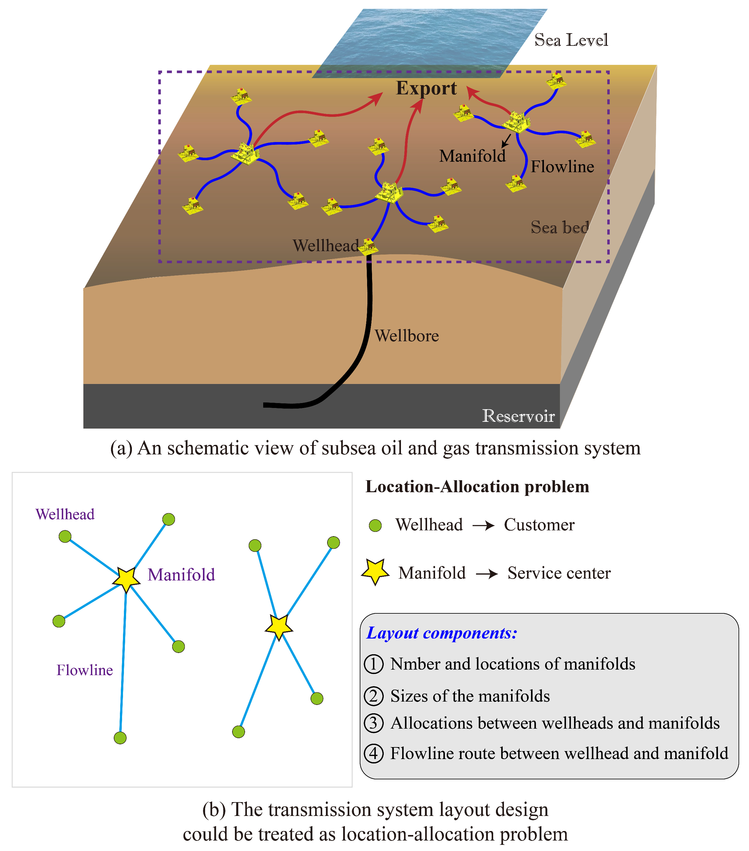
2.2. Problem Descriptions

Based on the proposed working structure shown in Figure 2 and the assumption, the mathematical problem can be described. Figure 4 helps to make the description.

As shown in Figure 4a, a set of customers is distributed on the $x-y$ plane, and the x and y coordinates are given. Each customer has its own production, with the demand for transportation shown. All production is transported to the service centers for the next stage of the operation. In Section 1, we indicate the four main tasks that should be completed to determine the optimal layout, as shown in Figure 1. The four tasks are shown below:

➀

Find the positions of the service centers;

➁

Select the size and capacity of the service centers from the available options;

➂

Determine the allocation between the customers and the service centers; in other words, determine which service center each customer should be connected to;

➃

Design the transportation routes between each customer and the corresponding service centers while considering the avoidance of obstacles distributed inside the target region;

Figure 4a–d illustrates the process of obtaining the expected layout through the proposed structure shown in Figure 2. The above four tasks are represented by decision variables in the proposed model, which is introduced in Section 4.

The objective is to minimize the total construction cost, including the cost of constructing the service centers and the cost of the transportation routes.

With the above objective and tasks to be determined, the production and subsea obstacles are considered restrictions that the subsea layout must satisfy. The constraints can be divided into three main types: connectivity constraints, functional constraints, and avoiding obstacle areas. Figure 5 provides an overview of the three types of constraints as well as the corresponding explanations.

Based on the above problem description and assumptions, the decision variables, objective, and the constraints can be quantified for the development of the layout optimization model, which is presented in detail in Section 3.

3. Mathematical Modeling

3.1. Parameter Definitions

To develop the mathematical model, according to the above description of the problem and the assumptions, the following parameters are defined:

(1)

The number of customers is $NC$, and the x and y coordinates are $(x_w^c,y_w^c)$, where $Q_w$ indicates the production rate of the $w^{th}$ customer, and $w=1,2,...,NC$, $IC$ denotes this node set.

(2)

The obstacle areas are treated as convex polygons, and all vertices’ coordinates are provided. The total number of obstacle area vertices is $NO$, and $IO$ denotes this node set;

(3)

The candidates of the service center positions. Coordinates $(x_k^s,x_k^s)$ indicate the $k^{th}$ service center candidates. The total number of candidates is $NS$, and $IS$ denotes this node set;

(4)

There are different types of service centers for selection. The total number of available types is $NSA$. For the $m^{th}$ type, $S{L}_m$ represents the maximum number of transportation routes it can host, and $Q{P}_m$ represents its production processing capacity. $P{S}_m$ denotes the corresponding cost;

(5)

The cost of the transportation route per unit length is $PR$;

(6)

All related nodes are gathered by order, forming a integrated node set represented by $IT$, $IT=[IO,IC,IS]$, and $NT$ denotes the element number. Obviously, $NT=NO+NC+NS$.

3.2. Decision Variables

As mentioned in Section 2, the four tasks for layout optimization are represented by the following set of five decision variables.

(1)

Binary variables $a_k$, where $a_k=1$ indicates that the $k_{th}$ service center candidate is selected; otherwise, $a_k=0$, $k=1,2,...,NS$. This decision variable set represents task ➀ defined in Section 2.

(2)

Binary variables $p_{k,m}$, where $p_{k,m}=1$ indicates that the $k_{th}$ service center uses the $m_{th}$ type from the available options; otherwise, $p_{k,m}=0$. $k=1,2,...,NS$, $m=1,2,...,NSA$. This decision variable set represents task ➀ defined in Section 2.

(3)

Binary variables $x_{i,j}$, where $x_{i,j}=1$, indicates that node i and node j are connected; otherwise, $x_{i,j}=0$. $i,j=1,2,...,NT$. This decision variable set represents task ➂ defined in Section 2.

(4)

Non-negative integer variables $c_{i,j}$, representing the number of route sections between node i and node j. $i,j=1,2,...,NT$. The decision variables are set considering the situation where there might be more than one route that passes through two consecutive nodes i and j, as illustrated in Figure 3.

(5)

Continuous non-negative variables $q_{i,j}$, denoting the total weight on the section between node i and j. $i,j=1,2,...,NT$. Decision variables $c_{i,j}$ and $q_{i,j}$ together represent task ➃ defined in Section 2.

In addition, there are two sets of auxiliary variables:

Adjacent matrix $v_{i,j}$. This is a $0-1$ matrix, indicating whether two nodes are immediately connectable, $i,j\in IT$. There are two rules for the determination of $v_{i,j}$. First, each node is not connectable with itself, which is $v_{i,i}=0$ for all $i\in IT$, $i=1,2,...,NT$. Second, if the section between node i and node j intersects with any one of the provided obstacle regions, they are not immediately connectable, and $v_{i,j}=0$; otherwise, $v_{i,j}=1$. In our previous work, the process of determining the adjacent matrix, including the method of recognizing the intersection between one section and obstacle polygons was developed, and detailed information can be seen in reference [30].

Distance matrix $d_{i,j}=1$, $i,j\in IT$. This matrix is used to include the distance between any two nodes. The Euclidean distance between node i and node j is applied if and only if $v_{i,j}=1$; otherwise, $d_{i,j}$ will be given a very large number for the convenience of mathematical modeling.

3.3. Objective Function

The objective of layout optimization is to minimize the total construction cost. As discussed above, the total cost consists of two parts: the first is the cost of the transportation routes, which is related to the length of the routes, and the other is the cost of the service centers, which is related to the selected types. Therefore, the objective function can be explicitly described using the decision variables, as shown in Equation (1).

$$\min \mathrm{TotalCost}=\sum _{i\in IT}\sum _{j\in IT}PR·d_{i,j}·c_{i,j}+\sum _{m=1}^{NSA}\sum _{k\in IS}{p}_{k,m}·P{S}_m$$

(1)

3.4. Constraints

Equations (2)–(22) make up of the constraints for the layout design in this work.

$$x_{i,j}\le v_{i,j},\forall i,j\in IT$$

(2)

$$x_{i,j}+x_{j,i}\le 1,\forall i,j\in IT$$

(3)

$$\mathrm{\Psi }{x}_{i,j}\le c_{i,j}\le \mathrm{\Phi }{x}_{i,j},\forall i,j\in IT$$

(4)

$$\mathrm{\Psi }{c}_{i,j}\le q_{i,j}\le \mathrm{\Phi }{c}_{i,j},\forall i,j\in IT$$

(5)

$$\sum _{j\in IT}{x}_{i,j}=1,\sum _{j\in IT}{x}_{j,i}=0,\forall i\in IC$$

(6)

$$\sum _{j\in IT}{c}_{i,j}=1,\sum _{j\in IT}{c}_{j,i}=0,\forall i\in IC$$

(7)

$$\sum _{j\in IT}{q}_{i,j}=Q_w,\sum _{j\in IT}{q}_{j,i}=0,\forall i\in IC,w=i-NO$$

(8)

$$\sum _{j\in IT}{x}_{i,j}\le 1,\forall i\in IO$$

(9)

$$\sum _{j\in IT}{c}_{i,j}-\sum _{j\in IT}{c}_{j,i}=0,\forall i\in IO$$

(10)

$$\sum _{j\in IT}{q}_{i,j}-\sum _{j\in IT}{q}_{j,i}=0,\forall i\in IO$$

(11)

$$\sum _{k=1}^{NS}{a}_k=NSD$$

(12)

$$\sum _{m=1}^{NSA}{p}_{k,m}=a_k,k=1,2,...,NS$$

(13)

$${\displaystyle \sum _{j\in IT}}{x}_{i,j}=0,\forall i\in IS$$

(14)

$$\left\{\begin{array}{c}{\displaystyle \sum _{j\in IT}}{x}_{j,i}\le {\displaystyle \sum _{m=1}^{NSA}}{p}_{k,m}·S{L}_m+\mathrm{\Phi }(1-a_k),\forall i\in IS\hfill \\ \hfill \\ {\displaystyle \sum _{j\in IT}}{x}_{j,i}\le \mathrm{\Phi }·a_k,\forall i\in IS\hfill \end{array}\right.$$

(15)

$$\sum _{j\in IT}{c}_{i,j}=0,\forall i\in IS$$

(16)

$$\left\{\begin{array}{c}{\displaystyle \sum _{j\in IT}}{c}_{j,i}\le {\displaystyle \sum _{m=1}^{NSA}}{p}_{k,m}·S{L}_m+\mathrm{\Phi }(1-a_k),\forall i\in IS\hfill \\ \hfill \\ {\displaystyle \sum _{j\in IT}}{c}_{j,i}\le \mathrm{\Phi }·a_k,\forall i\in IS\hfill \end{array}\right.$$

(17)

$$\sum _{j\in IT}{q}_{i,j}=0,\forall i\in IS$$

(18)

$$\left\{\begin{array}{c}{\displaystyle \sum _{j\in IT}}{q}_{j,i}\le {\displaystyle \sum _{m=1}^{NSA}}{p}_{k,m}·Q{P}_m+\mathrm{\Phi }(1-a_k),\forall i\in IS\hfill \\ \hfill \\ {\displaystyle \sum _{j\in IT}}{q}_{j,i}\le \mathrm{\Phi }·a_k,\forall i\in IS\hfill \end{array}\right.$$

(19)

$$\sum _{j\in IT}\sum _{i\in IS}{x}_{j,i}\le NC$$

(20)

$$\sum _{j\in IT}\sum _{i\in IS}{c}_{j,i}=NC$$

(21)

$$\sum _{j\in IT}\sum _{i\in IS}{q}_{j,i}=\sum _{w=1}^{NC}{Q}_w$$

(22)

Equations (2)–(5) set up the general constraints for the decision variables. Equation (2) indicates that nodes i and j cannot be connected as a route section unless they are immediately connectable; that is to say, $v_{i,j}=1$. Equation (3) shows that the route is single-directional. Equation (4) means that the route section between nodes i and j exists if and only if the two nodes are connected. Similarly, Equation (5) means that the transportation flow from nodes i to j exists if and only if there are route sections between them. The Greek signs $\mathrm{\Phi }$ and $\mathrm{\Psi }$ are given large and small numbers, respectively.

Equations (6)–(8) define the requirements that must be satisfied by the customer nodes. Customer nodes act as the sources, from which there are only routes starting, while no route arrives; thus, no transportation flow enters, as shown by the second terms from Equations (6)–(8). Starting from each customer, there is only one route, and the corresponding transportation flow rate going outside equals its production rate, as shown by the first terms in Equations (6)–(8). The third term defines the relationship between indexes w and i, based on the node arrangement proposed in Section 2.

Due to the need to avoid obstacles, the transportation routes might have some intermediate nodes which come from the vertices of the obstacle areas, as shown in Figure 6. Equations (9)–(11) show the requirements that these types of nodes must satisfy. Equation (9) indicates that there is, at most, one connection from node i to the other nodes. Equations (10) and (11) indicate that the route intervals and the transportation flow rate that enter and exist node i should satisfy the conservation relation.

Equation (12) means that the number of selected service centers must be equal to the designed number. Equation (13) defines the size selection rule, which is that for candidate k, if it is selected as the service center, only one size can be chosen.

The service centers are the terminals of the system, so there are no connections, no route sections, and no transportation flow rates from the service center candidates to the other nodes, as shown by Equation (14), Equation (16) and Equation (18), respectively.

As for the issues of entering the candidates of the service centers, first, the route sections that enter each candidate should not exceed the size that is selected from the available options. If candidate k is not selected, the number of entering route sections will be 0, obviously, as shown by Equations (15) and (17). Similarly, the transportation flow rate arriving at each candidate will be 0 if it is not selected; otherwise, the flow rate should not be larger than the processing capacity of the selected type, as shown by Equation (19).

Equation (20) means that the total number of connections toward all service center candidates should not exceed the number of customers. Equation (21) shows that the total number of route sections arriving at all service center candidates should be equal to the number of customers. According to Figure 3, there might be more than one route section between nodes, so we use the “≤” sign in Equation (20) and the “=” sign in Equation (21). Equation (22) indicates that the total flow rate transported to the service centers should be equal to the total production rate of the customers.

3.5. Short Summary of the Mathematical Model

Equations (1)–(22) consist of the layout optimization model, which belongs to the location-allocation problem considering obstacle areas and service center capacity restrictions. The decision variables, objective function, and constraints of the proposed model reflect the scenario described in Section 2. The total number of decision variables is $3{NT}^2+NS·NSA+NS$, including both integers and continuous variables. The total number of constraints is $4{NT}^2+6NC+2NO+10NS+4$. All objective functions and constraints are linear. Therefore, the proposed model is a mixed-integer linear programming model (MILP).

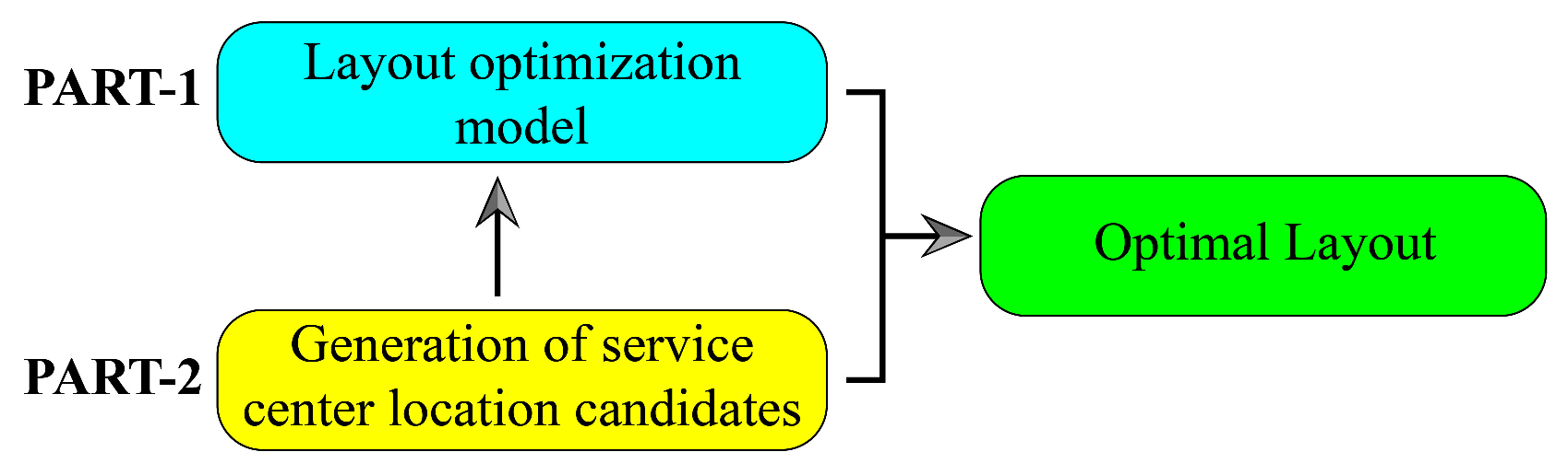
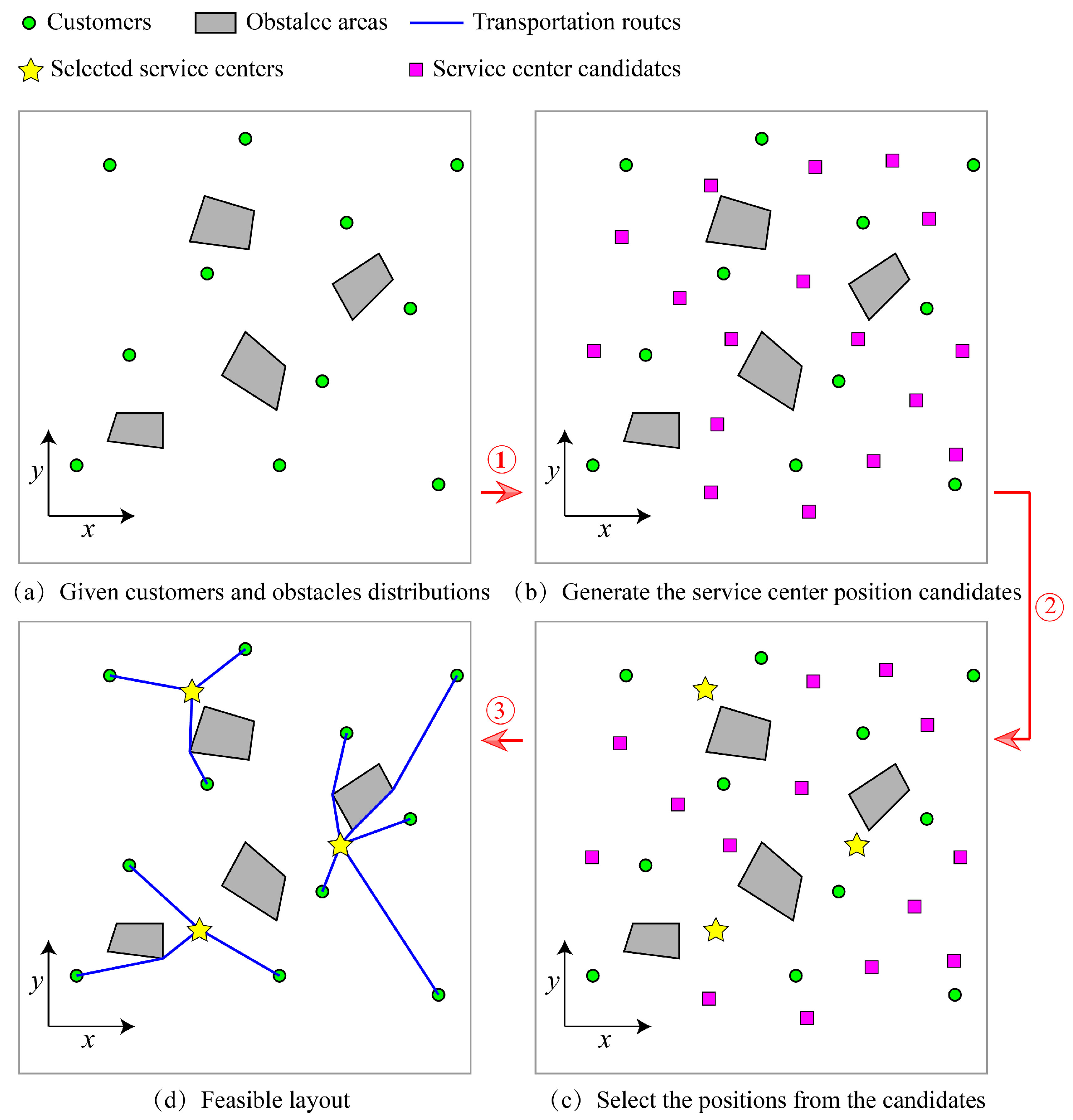
4. Solution Strategy

As indicated in Section 2, this work is divided into 2 parts, layout optimization modeling (Part-1) and the generation of service center location candidates (Part-2), which is shown in Figure 2. Part 1 was described in Section 3. Therefore, the subsequent step is to achieve Part-2, in which we have to answer a question: how can we generate the service center candidates? On one hand, in Section 1, the possibility of a “dimension explosion” brought about by the candidate distribution density was mentioned [31]. To avoid this issue, the amount of candidates should not be too large. On the other hand, the candidates should not be concentrated in a small area; instead, they should be distributed properly across the whole target area, thus contributing to the achievement of the global optimum (This is similar to the searching process of Simulated Annealing, through which the early period of searching is always performed with a big searching radius to ensure a global search performance [42]).

As a result, in this work, a solution strategy based on Delaunay triangulation focusing on generating the service center candidates considering both the global searching efficiency and the computational cost is proposed. Figure 7 helps to present the solution strategy.

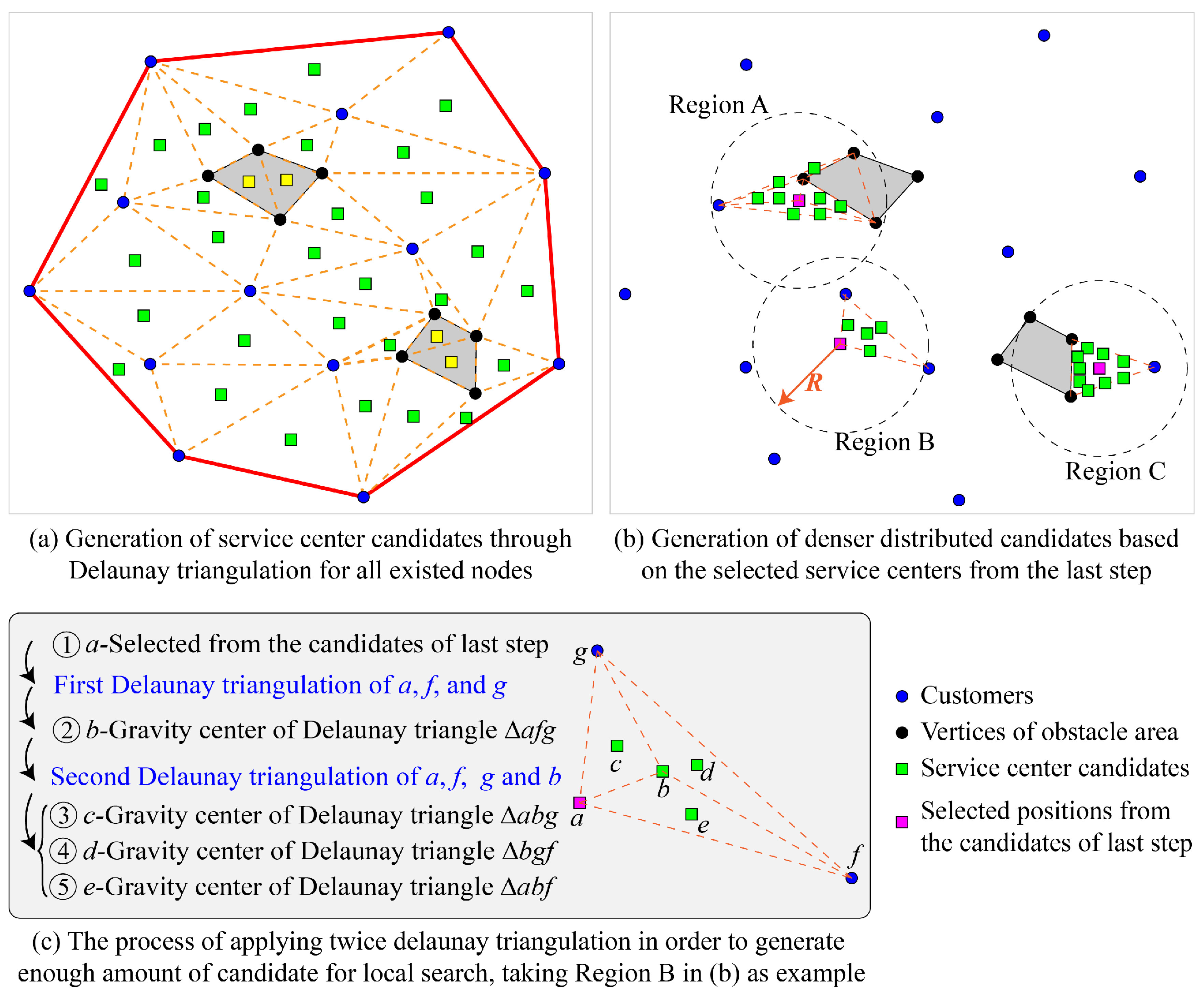
• Step 1: Delaunay triangulation is applied to the original node set, which includes the customer nodes and the vertices of the obstacle regions. Delaunay triangulation (also known as Delone triangulation) for a given set of discrete points in a plane is a triangulation such that no point is inside the circumcircle of any triangle [43]. The gravity centers of all Delaunay triangles, except for the ones inside the obstacles, are set as the service center candidates. Delaunay triangulation helps to make “uniformly” divisions of the target area, so that the distribution of the candidates is moderate, neither too dense (which might result in larger calculation consumption) nor too sparse (which might not bring a good solution), presenting the “global search” characteristics, as shown in Figure 7a. With these candidates, the proposed model can be solved through some linear programming solvers, such as CPLEX, GUROBI, etc. CPLEX is used in this work.
• Step 2: Centered at each obtained service center, the circle with a given radius R includes some of the existed nodes, which are collected and used to generate new candidates for the service centers. Delaunay triangulation is applied twice in order to provide denser candidates, as shown in Figure 7b,c. For each service center, the searching radius R comes from a given factor $\alpha$ and the minimum distance towards the other nodes. The factor $alpha$ is reduced proportionally after each step of local searching, thus resulting in a reduction in the search radius, as shown by Equation (23).

  $$\begin{array}{c}{R}_k^t={\alpha }^t·\min \{(x_k^S,y_k^S)-(x_i,y_i)\}\forall i\in NT\hfill \\ {\alpha }^{t+1}=\sigma ·{\alpha }^t\hfill \end{array}$$

  (23)

  This treatment generates candidates in a limited region which is closed to the service center positions obtained in the last step, presenting the “local search” characteristics, which helps to find more accurate service center positions. The updated MILP model results in a set of updated service center positions.
• Step 3: Reduce the given radius R proportionally, and repeat Step2 until the obtained service center positions do not change, thus achieving the final service center positions as well as the corresponding layout.

By applying the solution strategy, the proposed model is transformed to be a series of MILP models, starting from a global search, followed by a local search, thus finally converging to a high-quality solution.

5. Case Studies

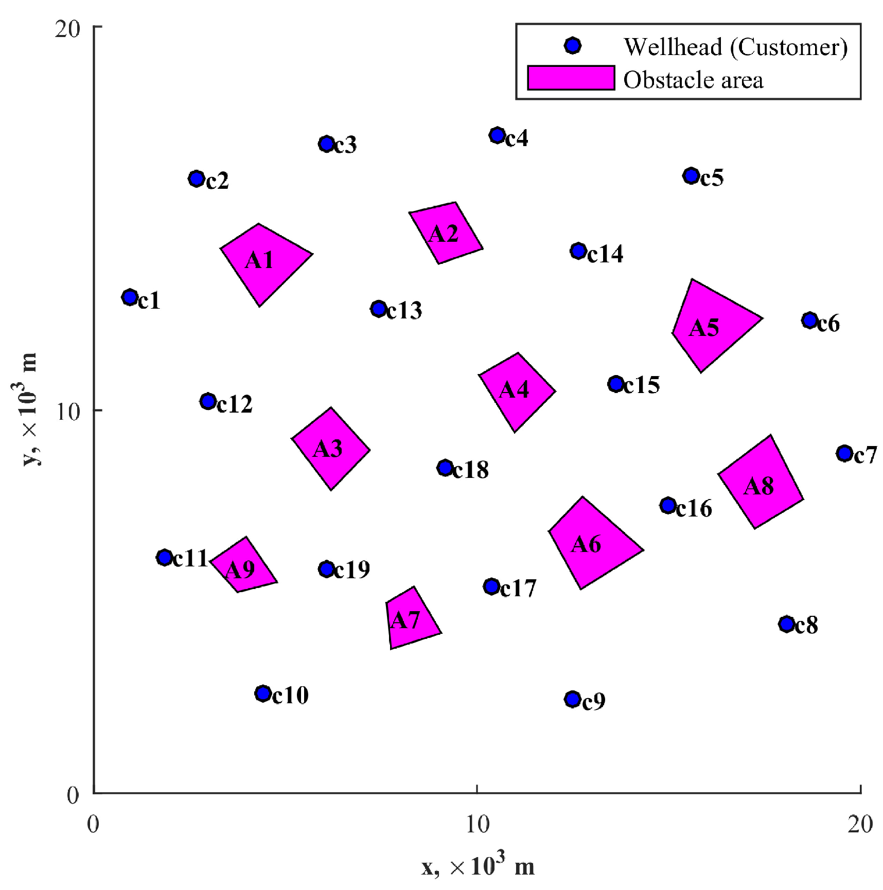
5.1. Input Information

In this work, an offshore oil field layout design is taken as the case study to show the application of the proposed model. In the offshore oil field, there are, in total, 19 subsea wells with varied production rates. The subsea wells act as the “customers”. Nine obstacle areas are distributed across the seabed, as shown in Figure 8. The coordinates of the wellheads as well as the obstacle area vertices are shown in

Table 1. Locations and production rates of the subsea wells.

Well No.	x-y Cord (m)	Flow Rate (${\mathbf{m}}^3$/day)	Well No.	x-y Cord (m)	Flow Rate (${\mathbf{m}}^3$/day)
1	(935.43, 12,909.21)	918.06	11	(1835.43, 6180.3)	1238.62
2	(2710.67, 16,027.38)	1407.18	12	(2983.15, 10,208.46)	1679.16
3	(6046.48, 16,979.12)	1368.48	13	(7404.75, 12,650.4)	1438.21
4	(10,513.49, 17,141.91)	1332.25	14	(12,656.17, 14,119.75)	1665.35
5	(15,603.91, 16,119.22)	1006.12	15	(13,601.6, 10,696.85)	1622.74
6	(18,642.47, 12,324.81)	1236.42	16	(14,959.86, 7486.84)	1855.76
7	(19,612.66, 8881.05)	1138.85	17	(10,377.25, 5391.36)	1317.39
8	(18,068.61, 4435.45)	1226.73	18	(9134.58, 8484.49)	1513.62
9	(12,519.93, 2435.98)	1100.93	19	(6046.48, 5879.75)	1110.49
10	(4436.37, 2598.78)	1177.61

and

Table 2. Distribution of the subsea obstacle areas.

Obstacle No.	Vertices’ Coordinates (m)	Obstacle No.	Vertices’ Coordinates (m)
A1	(3309.3, 14,211.58)	A6	(11,875.89, 6831.48)
	(4296.01, 14,862.76)		(12,747, 7741.47)
	(5703.82, 14,069.65)		(14,336.46, 6343.09)
	(4320.78, 12,696.32)		(12,701.59, 5320.4)
A2	(8234.57, 15,142.44)	A7	(7635.95, 4969.76)
	(9431.83, 15,422.12)		(8350.17, 5391.36)
	(10,146.06, 14,211.58)		(9064.4, 4180.82)
	(8994.21, 13,815.02)		(7751.54, 3763.4)
A3	(5171.24, 9252.55)	A8	(16,293.36, 8321.69)
	(6186.85, 10,066.54)		(17,655.76, 9348.56)
	(7198.33, 8952.01)		(18,506.23, 7670.51)
	(6186.85, 7904.27)		(17,238.78, 6902.44)
A4	(10,055.23, 10,905.56)	A9	(3032.69, 6042.55)
	(11,066.71, 11,489.96)		(3973.99, 6693.73)
	(12,036.9, 10,488.14)		(4783.17, 5508.24)
	(10,975.88, 9415.35)		(3746.92, 5249.44)
A5	(15,096.1, 11,999.22)
	(15,603.91, 13,418.47)
	(17,445.21, 12,395.77)
	(15,835.1, 10,976.53)

.

In order to collect the produced fluids from these wellheads, subsea manifolds are installed, and the wellheads are connected with the manifolds through a flowline. The flowline costs USD 2300/m. Subsea manifolds act as the “service center”. Available options with different sizes, prices, and processing capacities are shown in

Table 3. Available options for subsea manifolds.

Slot Number	Processing Capacity (bbl/day)	Price ($\times {10}^6$ USD)
4	35,000	10
6	50,000	12
8	65,000	16
10	80,000	20

. Four manifolds are designed to be installed.

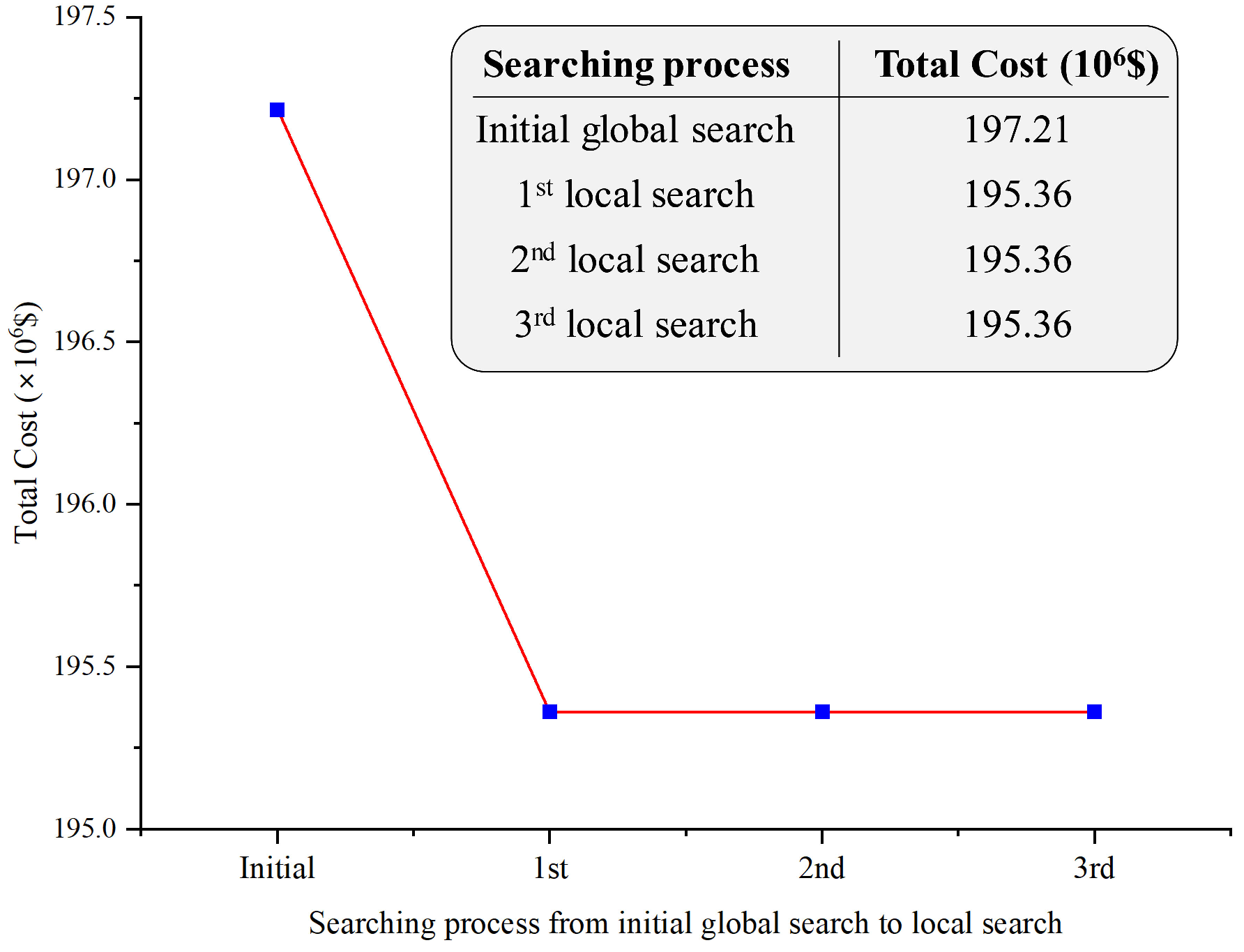
5.2. Optimization Results

Through the proposed model and the case input information, the optimal service center locations and the corresponding types, the allocations between wellheads and manifolds, as well as the flowline routes that connect wellheads and manifolds can be achieved by implementing the solution strategy proposed in Section 4.

First, all existing nodes, including the wellheads and vertices of obstacle areas, are included for Delaunay triangulation, thus generating the manifold location candidates, as shown in Figure 9. There are a total of 79 candidates, which are distributed across the whole area, presenting global characteristics.

Then, based on the generated manifold candidates, the proposed layout optimization model can be solved through the CPLEX solver, thus finishing Step 1,as indicated in Section 4. The optimized layout is shown in Figure 10a. The manifold locations are optimized from the given candidates distributed globally across the area, so that this process can be regarded as a global search. The optimization results are set as initial values for the subsequent further iteration process, which is shown in Step 2 and Step 3.

The local search radius factor $\alpha$ starts from 3, which means that, for each manifold, the searching radius will be 3 times the minimum distance toward the other nodes; therefore, the local search radius of each manifold will be different. Once the current local search has finished, $\alpha$ will be reduced proportionally by dividing by 1.2 ($\sigma =1.2$). Then, the updated $\alpha$ is used for the next local search. This process continues until the obtained manifold locations remain unchanged, as proposed in Section 4.

Figure 11 presents the process of the local search, in which we can find that, as the local search progresses, the searching area reduces, and the manifold positions converge to the optimal ones after three steps of local searching. The variation in the objective function value (total cost) is shown in Figure 12.

Figure 11 presents the process of the local search. As can be seen from the figure, the local search brings denser candidates, which are clustered around the initial manifold locations. This is good for searching possible better manifold locations, which are likely to be located close to the initial manifold locations through the global search. For instance, in Figure 11a, the newly generated candidates are closer to each other compared with Step 1, as shown in Figure 9, and a group of better manifold locations is achieved compared with the initial results, leading to a slight change in the layout. Under the updated manifold location, the searching radius is reduced by dividing 1.2 $\alpha$. In this way, more refined candidates are obtained around each manifold location, helping to search for possible better locations. The process is repeated until the manifold locations do not change, which means that there is no better location around the manifolds. In this case study, it is found that, from the second local search, the manifold locations remain stable, as shown in Figure 12, so the results are taken as the final solution.

Figure 10b shows the layout of final solution, and

Table 4. Comparison of the solutions to the initial global search and local search.

Items		Initial Layout from Global Search	Final Layout from Local Search
Manifold types and locations	M1	6 slots, (3438.66, 15,033.91)	6 slots (3476.43, 14,649.41)
	M2	6 slots, (14,621.33, 14,552.48)	6 slots, (13,194.25, 14164.58)
	M3	6 slots, (6193.73, 5050.46)	6 slots, (5971.56, 5469.9)
	M4	4 slots, (16,547.95, 5893.66)	4 slots, (16,547.95, 5893.66)
Cost of manifolds ($\times {10}^6$ $)		46	46
Cost of flowlines ($\times {10}^6$ $)		151.21	149.36
Total cost ($\times {10}^6$ $)		197.21	195.36

includes a comparison between the initial solution shown in Figure 10a and the final solution in Figure 10b. Both Figure 10a,b show that the flowline routes avoid the existing obstacle areas. In addition, the locations of manifolds, allocations of wellheads to the manifolds, and the selected sizes of the manifolds are all obtained, so the four tasks of layout optimization proposed in Section 2 are all completed.

Furthermore, from Table 4, we can observe that the solution strategy works, which reduces the total cost by USD 185 million compared with the initial global search. The total cost reduction results from the update of the manifold locations, which leads to shorter flowline lengths. The selection of manifold types and the allocations between wellheads and manifolds remain the same. Therefore, the proposed initial solution based on global Delaunay triangulation is of high quality, and the subsequent local search strategy could modify the manifold locations, bringing further optimization. The case study indicates the validity and feasibility of the proposed model as well as the solution strategy, which could effectively and correctly achieve the layout optimization for the subsea transmission network.

Compared with the orthogonal grid method mentioned in Section 1, the most significant point of the proposed model and solution strategy is the reduction of the manifold candidates, while the optimization results do not differ too much. This is because the optimization models are linear, which brings stable solutions, so that no matter which method of generating the manifold candidate is chosen, similar results will always be obtained as long as the proper grid density is selected. Therefore, comparing the effect of candidates on the model dimension is more meaningful. To display the difference more intuitively, the candidates achieved through Delaunay triangulation in Figure 9 are set as the baseline, and an orthogonal grid with a similar grid density is generated, as shown in Figure 13. For our case, there are 79 candidates, resulting in 54,263 decision variables and 72,804 constraints, while for the orthogonal grid case, there are 97 candidates, resulting in 69,797 decision variables and 93,576 constraints, so that the reduction of 18 candidates leads to decreases of 15,534 decision variables and 20,772 constraints, which significantly reduces the calculation consumption. Although the orthogonal grid in Figure 13b was generated roughly, the dimension comparison provides a qualitative view of the efficiency advantage of the proposed method of generating manifold location candidates based on Delaunay triangulation.

5.3. Effect of Manifold Number

In in the above case study, the designed manifold number is four. Different manifold numbers will bring different layouts, as well as different total costs. To quantify such differences, based on the proposed model, the designed manifold number is changed from three to seven. The layout under each manifold number as well as the corresponding cost is shown in Figure 14.

As shown in Figure 14f, given different manifold numbers, the optimized layouts turn out to be different. With the increase in the manifold number, the flowline cost decreases, while the manifold cost increases, leading to a decrease in the total cost. This is because more manifolds lead to fewer wells being allocated to one manifold, making the required manifold sizes smaller. Though a smaller manifold is cheaper, an increased number still leads to a higher manifold cost. At the same time, having more manifolds leads to a shorter flowline length, which can be observed in Figure 14a–e, so the cost of the flowline is reduced. The reduction magnitude in the flowline cost is larger than the increment magnitude of the manifold; therefore, the total cost decreases.

Figure 15 presents a more detailed cost decomposition and also presents the cost variation trend described above. Furthermore, we find that the cost of flowline occupies more that 50% of the total cost. Therefore, the measurements related to reducing the flowline cost will be more effective for reducing the total cost, for example, lowering the flowline price per unit length by using cheaper material as long as the safety issues and engineering requirements can be ensured.

We should note that the above cost analysis is closely related to the given information, and under different given flowline prices and manifold prices, there might be some different results. However, this part of the work brings some inspiration for investment management related to the subsea layout design and shows one of the possible applications of the proposed model, indicating its flexibility.

6. Conclusions

This paper proposed a layout optimization model based on mixed-integer linear programming for a subsea transmission network with lined-shaped structures, such as a subsea pipe system for an offshore field or a subsea power cable network for a offshore wind power system, etc., aimed at minimizing the total layout cost. Through the proposed model, the locations of service centers, the allocations between customers and service centers, as well as the transmission routes that avoid subsea obstacles can all be figured out.

An offshore field with 19 wells was taken as the case study, indicating the validity, feasibility, and stability of the proposed model and the solution strategy. Additionally, the effects of the manifold number on the layout optimization and the cost components were analyzed. The variation in the total cost is the trade-off for having different cost items, inferring that focusing on the cost reduction of key items might have a more positive influence on investment management. The analysis also shows one of the possible applications of the proposed model, indicating its flexibility

There are two main contributions in this work. First, production requirements and the avoidance of subsea obstacles are both integrated into the MILP model quantitatively and directly, making the description of the layout closer to practical situations. Second, a “global to local” search process based on the Delaunay triangulation method is constructed to solve the model, instead of the orthogonal grid method, which reduces the number of service center candidates, providing an effective method of finding the optimal solution with a high efficiency.

For the proposed model and the solution strategy, there are also some limitations that need further improvements. The production rates of the customers are assumed to be fixed, while in practical situations, production might vary with time, presenting volatility and uncertainty, which will influence the model’s development. Additionally, energy consumption along the transmission routes is not taken into consideration, which will also affect the layout optimization. Including these complex conditions in the layout design will make the optimization result closer to the practical situation, thus obtaining higher practical value, but at the same time, the mathematical model will be more complicated. These issues will be considered in our future work.

References

1. Buckley, K.; Uehara, R. Subsea Concept Alternatives for Brazilian Pre-Salt Fields. In Proceedings of the Offshore Technology Conference Brasil, Rio de Janeiro, Brazil, 24–26 October 2017. [Google Scholar] [CrossRef]
2. Froese, G.; Ku, S.Y.; Kheirabadi, A.C.; Nagamune, R. Optimal layout design of floating offshore wind farms. Renew. Energy 2022, 190, 94–102. [Google Scholar] [CrossRef]
3. Almedallah, M.K.; Walsh, S.D. Integrated well-path and surface-facility optimization for shallow-water oil and gas field developments. J. Pet. Sci. Eng. 2019, 174, 859–871. [Google Scholar] [CrossRef]
4. Cocimano, R. KM3NeT deep-sea cabled network: The star-like layout. Nucl. Instruments Methods Phys. Res. Sect. A Accel. Spectrom. Detect. Assoc. Equip. 2013, 725, 223–226. [Google Scholar] [CrossRef]
5. Liu, H.; Gjersvik, T.B.; Faanes, A. Subsea field layout optimization (part II)–the location-allocation problem of manifolds. J. Pet. Sci. Eng. 2022, 208, 109273. [Google Scholar] [CrossRef]
6. Cooper, L. Location-Allocation Problems. Oper. Res. 1963, 11, 331–343. [Google Scholar] [CrossRef]
7. Chu, P.C.; Beasley, J.E. A genetic algorithm for the generalised assignment problem. J. Oper. Res. Soc. 1997, 48, 804–809. [Google Scholar] [CrossRef]
8. Farahani, R.Z.; Hekmatfar, M.; Fahimnia, B.; Kazemzadeh, N. Hierarchical facility location problem: Models, classifications, techniques, and applications. Comput. Ind. Eng. 2014, 68, 104–117. [Google Scholar] [CrossRef]
9. Şahin, G.; Süral, H.; Meral, S. Locational analysis for regionalization of Turkish Red Crescent blood services. Comput. Oper. Res. 2007, 34, 692–704. [Google Scholar] [CrossRef]
10. Shariff, S.; Moin, N.H.; Omar, M. Location allocation modeling for healthcare facility planning in Malaysia. Comput. Ind. Eng. 2012, 62, 1000–1010. [Google Scholar] [CrossRef]
11. Mestre, A.M.; Oliveira, M.D.; Barbosa-Póvoa, A.P. Location-allocation approaches for hospital network planning under uncertainty. Eur. J. Oper. Res. 2014, 240, 791–806. [Google Scholar] [CrossRef]
12. Cicek, C.T.; Gultekin, H.; Tavli, B. The location-allocation problem of drone base stations. Comput. Oper. Res. 2019, 111, 155–176. [Google Scholar] [CrossRef]
13. Feng, Y.; Liu, Y.K.; Chen, Y. Distributionally robust location–allocation models of distribution centers for fresh products with uncertain demands. Expert Syst. Appl. 2022, 209, 118180. [Google Scholar] [CrossRef]
14. Fahmy, S.A.; Zaki, A.M.; Gaber, Y.H. Optimal locations and flow allocations for aggregation hubs in supply chain networks of perishable products. Socio-Econ. Plan. Sci. 2022, 86, 101500. [Google Scholar] [CrossRef]
15. Wang, Z.; Zhang, J. A task allocation algorithm for a swarm of unmanned aerial vehicles based on bionic wolf pack method. Knowl.-Based Syst. 2022, 250, 109072. [Google Scholar] [CrossRef]
16. Zhang, J.; Li, X.; Jia, D.; Zhou, Y. A Bi-level programming for union battery swapping stations location-routing problem under joint distribution and cost allocation. Energy 2023, 272, 127152. [Google Scholar] [CrossRef]
17. Devine, M.D.; Lesso, W.G. Models for the Minimum Cost Development of Offshore Oil Fields. Manag. Sci. 1972, 18, 378–387. [Google Scholar] [CrossRef]
18. Wang, Y.; Duan, M.; Xu, M.; Wang, D.; Feng, W. A mathematical model for subsea wells partition in the layout of cluster manifolds. Appl. Ocean Res. 2012, 36, 26–35. [Google Scholar] [CrossRef]
19. Wang, Y.; Duan, M.; Feng, J.; Mao, D.; Xu, M.; Estefen, S.F. Modeling for the optimization of layout scenarios of cluster manifolds with pipeline end manifolds. Appl. Ocean Res. 2014, 46, 94–103. [Google Scholar] [CrossRef]
20. Liu, H.; Gjersvik, T.B.; Faanes, A. Subsea field layout optimization (part III) — the location-allocation problem of drilling sites. J. Pet. Sci. Eng. 2022, 208, 109336. [Google Scholar] [CrossRef]
21. Fischetti, M.; Pisinger, D. Optimizing wind farm cable routing considering power losses. Eur. J. Oper. Res. 2018, 270, 917–930. [Google Scholar] [CrossRef] [Green Version]
22. Liu, Y.; Fu, Y.; Huang, L.L.; Ren, Z.X.; Jia, F. Optimization of offshore grid planning considering onshore network expansions. Renew. Energy 2022, 181, 91–104. [Google Scholar] [CrossRef]
23. Kim, S.; Kang, S.; Lee, J.H. Optimal design of offshore wind power farm in high resolution using geographical information system. Comput. Chem. Eng. 2023, 174, 108253. [Google Scholar] [CrossRef]
24. Ramshani, M.; Ostrowski, J.; Zhang, K.; Li, X. Two level uncapacitated facility location problem with disruptions. Comput. Ind. Eng. 2019, 137, 106089. [Google Scholar] [CrossRef]
25. Kratica, J.; Dugošija, D.; Savić, A. A new mixed integer linear programming model for the multi level uncapacitated facility location problem. Appl. Math. Model. 2014, 38, 2118–2129. [Google Scholar] [CrossRef]
26. Gokbayrak, K.; Kocaman, A.S. A distance-limited continuous location-allocation problem for spatial planning of decentralized systems. Comput. Oper. Res. 2017, 88, 15–29. [Google Scholar] [CrossRef]
27. Rodrigues, H.W.L.; Prata, B.A.; Bonates, T.O. Integrated optimization model for location and sizing of offshore platforms and location of oil wells. J. Pet. Sci. Eng. 2016, 145, 734–741. [Google Scholar] [CrossRef] [Green Version]
28. Silva, L.M.; Guedes Soares, C. Oilfield development system optimization under reservoir production uncertainty. Ocean Eng. 2021, 225, 108758. [Google Scholar] [CrossRef]
29. Nash, I. Arctic Development of the Canadian Beaufort Sea, Geohazards and Export Route Options. In Proceedings of the OTC Arctic Technology Conference, Copenhagen, Denmark, 23–25 March 2015. [Google Scholar] [CrossRef]
30. Hong, C.; Estefen, S.F.; Lourenço, M.I.; Wang, Y. A nonlinear constrained optimization model for subsea pipe route selection on an undulating seabed with multiple obstacles. Ocean Eng. 2019, 186, 106088. [Google Scholar] [CrossRef]
31. Zhang, H.; Liang, Y.; Ma, J.; Qian, C.; Yan, X. An MILP method for optimal offshore oilfield gathering system. Ocean Eng. 2017, 141, 25–34. [Google Scholar] [CrossRef]
32. Wu, Y.; Xia, T.; Wang, Y.; Zhang, H.; Feng, X.; Song, X.; Shibasaki, R. A synchronization methodology for 3D offshore wind farm layout optimization with multi-type wind turbines and obstacle-avoiding cable network. Renew. Energy 2022, 185, 302–320. [Google Scholar] [CrossRef]
33. Hong, C.; Estefen, S.F.; Wang, Y.; Lourenço, M.I. Mixed-integer nonlinear programming model for layout design of subsea satellite well system in deep water oil field. Autom. Constr. 2021, 123, 103524. [Google Scholar] [CrossRef]
34. Mikolajková, M.; Haikarainen, C.; Saxén, H.; Pettersson, F. Optimization of a natural gas distribution network with potential future extensions. Energy 2017, 125, 848–859. [Google Scholar] [CrossRef]
35. Mikolajková, M.; Saxén, H.; Pettersson, F. Linearization of an MINLP model and its application to gas distribution optimization. Energy 2018, 146, 156–168. [Google Scholar] [CrossRef]
36. Gong, D.; Gen, M.; Xu, W.; Yamazaki, G. Hybrid evolutionary method for obstacle location-allocation. Comput. Ind. Eng. 1995, 29, 525–530. [Google Scholar] [CrossRef]
37. Gong, D.; Gen, M.; Yamazaki, G.; Xu, W. Planar Location-allocation with Obstacles Problem. 1996 IEEE Int. Conf. Syst. Man Cybernetics. Inf. Intell. Syst. 1996, 4, 2671–2676. [Google Scholar]
38. Hong, C.; Estefen, S.F.; Wang, Y.; Lourenço, M.I. An integrated optimization model for the layout design of a subsea production system. Appl. Ocean Res. 2018, 77, 1–13. [Google Scholar] [CrossRef]
39. Dutta, R.N.; Ghosh, S.C. Mobility aware resource allocation for millimeter-wave D2D communications in presence of obstacles. Comput. Commun. 2023, 200, 54–65. [Google Scholar] [CrossRef]
40. Lerch, M.; De-Prada-Gil, M.; Molins, C. A metaheuristic optimization model for the inter-array layout planning of floating offshore wind farms. Int. J. Electr. Power Energy Syst. 2021, 131, 107128. [Google Scholar] [CrossRef]
41. Saint-Marcoux, J.; Legras, J. Impact on Risers and Flowlines Design of the FPSO Mooring in Deepwater and Ultra Deepwater. In Proceedings of the OTC Offshore Technology Conference, Houston, TX, USA, 5–8 May 2014. [Google Scholar] [CrossRef]
42. Kirkpatrick, S.; Gelatt, C.D.; Vecchi, M.P. Optimization by Simulated Annealing. Science 1983, 220, 671–680. [Google Scholar] [CrossRef]
43. Sastry, S.P. A 2D advancing-front Delaunay mesh refinement algorithm. Comput. Geom. Theory Appl. 2021, 97, 101772. [Google Scholar] [CrossRef]
Figure 1. An schematic view of a subsea transmission system for an offshore oil field.
Jmse 11 01171 g001
Figure 2. The structure of finding out the optimal layout for the subsea transmission network.
Jmse 11 01171 g002
Figure 3. Simplification of the situation where multiple routes are parallel or close to each other.
Jmse 11 01171 g003
Figure 4. Brief description of the treatment of the layout design process.
Jmse 11 01171 g004
Figure 5. Descriptions of the constraints that the layout optimization must satisfy.
Jmse 11 01171 g005
Figure 6. An schematic illustration in which the obstacle area vertices act as the intermediate nodes of the transportation routes in order to avoid the obstacle area.
Jmse 11 01171 g006
Figure 7. A schematic illustration of the solution strategy.
Jmse 11 01171 g007
Figure 8. Distribution of the subsea wellheads and the obstacles.
Jmse 11 01171 g008
Figure 9. Delaunay triangulation and the generated manifold location candidate for the global search.
Jmse 11 01171 g009
Figure 10. The layouts under the initial global search and local search.
Jmse 11 01171 g010
Figure 11. The manifold candidates and corresponding optimized layouts under different local search steps.
Jmse 11 01171 g011
Figure 12. The variation in the total cost from the initial global search to the local search.
Jmse 11 01171 g012
Figure 13. Comparison of the manifold candidate distribution under Delaunay triangulation and the orthogonal grid.
Jmse 11 01171 g013
Figure 14. Layouts and cost comparison under different manifold numbers.
Jmse 11 01171 g014
Figure 15. Cost decomposition under different manifold numbers.
Jmse 11 01171 g015